Article

Evaluating Presence Data versus Expert Opinions to Assess Occurrence, Habitat Preferences and Landscape Permeability: A Case Study of Butterflies

1
Department of Conservation Biology, UFZ—Helmholtz Centre for Environmental Research, Permoserstr. 15, 04318 Leipzig, Germany
2
Department of Biology, Lund University, Sölvegaten 37, 22362 Lund, Sweden
3
iDiv—German Centre for Integrative Biodiversity Research, Halle-Jena-Leipzig, Deutscher Platz 5e, 04103 Leipzig, Germany
4
Department of Community Ecology, UFZ—Helmholtz Centre for Environmental Research, Theodor-Lieser-Str. 4, 06120 Halle, Germany
*
Authors to whom correspondence should be addressed.
Environments 2018, 5(3), 36; https://doi.org/10.3390/environments5030036
Submission received: 9 February 2018 / Revised: 22 February 2018 / Accepted: 26 February 2018 / Published: 28 February 2018

Abstract

:
We explored how presence data and expert opinions performed with respect to identifying the ecological preferences and the spatial needs of six butterfly species in the Federal State of Saxony, Germany. We used presence records and a land-cover map. In parallel we used expert responses to evaluate the 40 land-cover types occurring in the map, in terms of both suitability and permeability for the six species. Presence data were translated into preferences through Ivlev’s electivity indices (IEI). Visual analysis of preference maps based on IEI showed a distinct pattern of suitable versus less suitable areas. Similarly, spatial analyses found that presence-points were closer to suitability areas based on IEI than those that were based on expert data. However, in case of mismatches between expert and presence-based evaluations, independent experts identified the expert evaluation as better and considered IEI outcomes as wrong. We found a medium to high correlation between land-cover class suitability and permeability based on expert opinions for all species. This indicates that expert evaluation of permeability is affiliated with habitat suitability. Integration of species-presence data and expert-knowledge about species could enhance our capabilities to understand and potentially map suitability while gathering information about suitability and permeability separately can improve species conservation planning.

1. Introduction

Biodiversity conservation has become a core issue in research and policy due to the recognition of the magnitude of anthropogenic and environmental threats [1]. Failures in achieving the 2010 goals of the Convention on Biological Diversity to slow down the loss of biodiversity, and the setting of new biodiversity targets for 2020, stress an urgent need to expand the current reserve networks and to improve their effectiveness in protecting species and habitats [2]. To facilitate the spatial selection of areas for conservation in a transparent way, a number of methods have been developed [3,4]. Such methods require comprehensive biological databases, especially with respect to species distribution, occurrence, and abundance in different environments. Furthermore, underlying data need to be up to date, sufficiently accurate, detailed, and in a resolution that reflects the environmental requirements of the species or habitats in question [5,6,7]. Such data, at the required level of resolution and detail, are rarely available [8,9,10]. Consequently, most strategies for the spatial design of nature conservation efforts depend on incomplete and biased distribution databases [11,12]. This could negatively affect conservation efforts by causing non-optimal performance in identifying priority areas for conservation [13,14,15].
Wildlife habitat selection models [16], habitat suitability models, and maps that are derived from them, are among the most broadly used tools for identifying the ecological needs of species [17]. They rely on presence only, presence-absence, or abundance data with the former being the most commonly available type of data [18,19]. However, obtaining reliable species occurrence data may be difficult, for instance, because data collection methods are often either non-standardized or even unknown [20,21,22]. It is increasingly acknowledged that landscape permeability should be another important aspect for conservation planning. Permeability is critical for species’ survival in human-altered environments, as it affects the movements of animals across landscapes, and hence their probability to survive in small, otherwise-isolated populations [23,24]. Suitability and permeability are therefore two central aspects in determining the survival of species in patchy landscapes. But these two should not be mixed with each other, as they describe different species-specific attributes. Habitat suitability describes the extent of environmental elements that are required for supporting individual and population persistence. It could be defined along a continuum from low to high, but it should also be perceived as a multidimensional set of variables that depend on the type of resources that are needed, at a given life stage or state, for various functions: survival, reproduction, and population maintenance [25,26,27]. Permeability, on the other hand, is defined as “the degree to which regional landscapes, encompassing a variety of natural, semi-natural and developed land cover types, are conducive to wildlife movement and sustain ecological processes” [28]. Permeability is a measure of animal-landscape interactions, determined by landscape structure, the tendency to move into (and through) different environments, and the risk of mortality in each of those. Consequently, a range of empirical studies demonstrate that environments that are “unsuitable” for daily functions may be highly permeable for dispersers. A landscape can be highly permeable, but if animals prefer to stay in elements of such a landscape, the average rate of dispersal would be very low, even if they move a lot, and thus show high movement activity. If they prefer to leave, dispersal speed would probably be similar to the level of movement [29,30,31]. The individual movement can be reduced either due to “mechanical” reasons (e.g., grassland species moving through forest) or the permeability regarding population dispersal can be reduced because of an increasing mortality (lack of connectivity and landscape resistance). To obtain reliable estimates of permeability, one therefore needs information both on the movement capacities of species, their movement decisions in different environments (i.e., both preference and diffusion rates), and indications of habitat-specific mortality rates. This requires intensive research using telemetry or CMR (Capture-Mark-Recapture) that is expensive, and therefore available only for few species [32]. Consequently, knowledge gaps are particularly large with respect to permeability. One means to overcome gaps in knowledge, for both suitability and permeability, could be to rely on expert knowledge in order to gain a better understanding of species-habitat relationships [33,34]. Especially, opinions about species-habitat relationships serve as baseline knowledge for planning of conservation projects, but are rarely tested empirically [35,36,37,38,39].
Here, we explored the question of how presence data and expert opinions perform with respect to identifying the ecological needs of six butterfly species in the Federal State of Saxony, Germany. We particularly focused on differentiating suitability (or proxies for it) from permeability. Butterflies were chosen because they are commonly used as bio-indicators for ecological trends and for advancing conservation theory and practice [40,41,42], data are readily available through rapidly expanding monitoring efforts [43], and a relatively large number of experts can be consulted.
To complement presence data originating from monitoring efforts which could only offer information on habitat preferences of species, evaluations of both preferences and permeability from six experts have been incorporated. Thereby, we aimed at (a) developing maps that separate habitat preferences from permeability, (b) comparing the outcomes of empirical-based versus expert-opinion based analyses, (c) identifying matches and mismatches between expert-opinion and empirical-data, and (d) proposing insights into what can be learned from each knowledge-source.

2. Materials and Methods

2.1. Study Area

The study was conducted using data from the Federal State of Saxony, in central-east Germany (circa 18,500 km²). The most dominant land-cover in Saxony is arable fields, while one-fourth of the state area is forested. Grasslands and extensive agricultural practices comprise additional important proportions [44]. The climate is temperate warm and slightly humid, with cool winters and warm summers and colder conditions in the mountain areas, primarily in the south, bordering the Czech Republic (Ore Mountains, up to circa 1200 m) [45]. The average annual precipitation ranges from circa 650 mm in the north-west to 900 mm at the higher altitudes in the south. Average annual temperature follows the same spatial pattern, declining from 8.58 °C in the north-west to 7.58 °C in the south-east [46].

2.2. Species Data

Point presence data were used for six butterfly species: Purple Emperor (Apatura iris, Nymphalidae), Grayling (Hipparchia semele, Nymphalidae), Large Copper (Lycaena dispar, Lycaenidae), Large Tortoiseshell (Nymphalis polychloros, Nymphalidae), Dusky Large Blue (Phengaris nausithous, Lycaenidae) and Silver-studded Blue (Plebejus argus, Lycaenidae). These species differ in their distribution and commonness, as well as in terms of habitat requirements and their movement distances. The conservation status of Hipparchia semele is defined as “least concern”, while Lycaena dispar and Phengaris nausithous are categorized under lower risk and “near threatened” categories, respectively. The remaining species are not listed in relevant red lists of threatened species, but all are of conservation concern for the state of Saxony, Germany [47,48,49,50].
Data were originated from opportunistic observations collected with an accuracy of 1 km. Data was available from the more distant past, but due to land-use changes in the region following Germany’s reunification, as well as for consistency with the land-cover map available (see below), our analyses were based only on presence records from the years 2000–2008. Since observations were not conducted systematically, the data were regarded as “presences” only, and absence data were considered unavailable.

2.3. Land-Cover Data

Land cover data set includes detailed vegetation and land-use patterns for the Federal State of Saxony, Germany. The data set were characterized based on aerial photos taken in 2005 by the Saxon State Agency for Environment, Agriculture and Geology (LfULG) [51]. The 40 land use classes in the BTLNK (Biotoptypen- und Landnutzungskartierung) data set can be displayed, from general (eight classes) to most detailed (See Appendix A). The BTLNK data set was preferred over CORINE (coordination of information on the environment) land cover due to more detailed classification and spatial accuracy. The land cover data set can be used to identify habitat suitability and permeability of six butterfly species.

2.4. Data Preparation and Analysis

To link the butterflies’ presence data with the land-cover map, one must consider the coarse spatial resolution of the observation data (1 × 1 km²). We therefore overlaid the presence data on a 1 km by 1 km grid. The grid was used to generate points based on the coordinates of the grid cells’ centers. We then calculated the proportion of each land cover class over all 1 km2 grid cells, and again for all of the occupied grid cells for each species. We included in the analyses only 1 km2 cells that fell completely within the borders of Saxony.
To assess the suitability of the various land-cover types, we applied two methods for calculating Ivlev’s Electivity Index [52]. This index was originally developed to describe the food preferences of predatory species by calculating the mean amount of the prey organism in the landscape and comparing it to the observed amount of prey taken up by the predator. Later on, the index was adopted for habitat preference calculation, where it can be used to compare how observations of a given species relate to the distribution of available land-cover types, or habitats, in a given landscape [53,54], Ivlev’s index is calculated as:
E i = r i p i r i + p i
where, r reflects the observed occurrence and p reflects the proportional availability of a given land-cover type for each of the i habitats. The outcome, Ei, varies from −1.0 to +1.0, where positive values indicate preferred (i.e., suitable) habitats, negative values denote avoidance (i.e., unsuitable) and Ei (IEI) = 0 indicates no preference [52,54]. We calculated the index in two ways that reflect different scales of information resolution: In the first approach, we considered information regarding the total number of occupied cells in a given land-cover class, ri being the relative proportion of number of occupied cells of a given land-cover where butterflies were recorded, and pi being the relative proportion of number of occupied cells of a given land-cover in the whole of Saxony. Here, the most dominant habitat type is assigned to each cell. In the second approach, which considers the abundance of different land-cover types within each of the 1 km cells, ri was the relative proportion of all the land cover classes occurring within all 1 km grid cells where a butterfly has been recorded, and pi was the relative proportion of land cover classes in all 1 km grid cells in Saxony. In the following, we call the former index IEIoccup and the latter one IEIabund. To assess, whether the abundance or rarity of a certain land-cover may result in higher IEI value or variance, we correlated both indices with the abundance of land cover classes within 1 km squares. Calculations and statistical analysis were performed using Microsoft Excel 2007 (Microsoft, Redmond, WA, USA).

2.5. Expert Opinions on Suitability and Permeability

To obtain independent information on land cover class suitability and permeability, we contacted about 70 butterfly experts to ask if they were willing to assign values for each of the six butterfly species. Experts could rank land-covers from one to four, where 1 would denote either “very suitable habitat” or, respectively, very high permeability, and 4 denotes highly unsuitable as habitat or, respectively, very low permeability. Out of the experts contacted, six replied and returned a table with estimates for habitat suitability and permeability for all of the 40 land-cover types and all species. We derived the average values and variance from the six expert opinions for each land-cover with species combination. The average values were then adjusted to the same range of Ivlev’s electivity index, from −1 (non-preferred) to +1 (preferred) [52] using a linear function (y = ax + b). We compared the average land cover class suitability of expert opinions and variance between all expert opinions to detect whether there is a certain systematic bias in the answers provided by experts. We then tested for correlation between expert opinion on permeability and habitat suitability based on both IEI and expert opinion to understand their relationships.

2.6. Preparation of Maps

Maps based on land cover class preferences (from both IEI and experts opinions) were generated by assigning the identified suitability values to the vector map of the biotope and land cover (BTLNK). Presence data for the six butterfly species originated from records during the years 2000–2008 was used to generate points in ArcMap based on their respective co-ordinates. Following number of presence points found for each species: A. iris (69), H. semele (65), L. dispar (51), N. polychloros (37), P. nausithous (200), and P. argus (49). Later, these vector maps and presence points were used in “point to polygon” analysis for distance investigation. Further, maps were then up-scaled to create a second raster map with a resolution of 1 by 1 km, so that suitability maps and the presence-points would have the same spatial resolution. Conversion of the vector maps to raster was performed by using the tool “polygon to raster” (Arc Toolbox, ArcGIS 10.1, Esri, Redlands, CA, USA) [55]. Each 1 km2 cell was assigned the land cover type value based on “maximum combined area” (i.e., the most dominant land-cover type). We used the “maximum combined area” approach to represent dominant land cover. Presence-points of species were overlaid on the 1 km2 cell resolution raster maps for visual assessment.

2.7. Comparison of Expert Opinions and Ivlev’s Electivity Indices

We compared habitat suitability based on IEI versus expert opinions to assess their respective performance. The following methods were used for comparison: (1) Visual assessment of the habitat suitability maps to identify general patterns of suitability in Saxony; and, (2) In spatial analysis, presence points were overlaid on polygon maps of habitat preference (based on IEI and expert opinions) to calculate distance from the nearest preferred area (IEI values > 0). Here, the assumption was that a small distance should represent a spatial matching between observations and the areas defined as suitable. Higher number of occupied cells in preferred area and shorter average distance of presence-points from preferred area should represent better prediction of preferred suitable area; (3) Finally, we compared the preference values based on IEI versus expert opinions for each of the 40 land-cover types, to identify the correlation levels as well as specific matches and mismatches (also with respect to land-cover rarity). The matches and mismatches provided additional information that was sent back to the experts for re-assessment and remarks about initial outcomes.

2.8. Evaluation of Habitat Preference Results by Experts

Once completing the analyses, we contacted all six experts again to discuss habitat preference outcomes. These experts, as well as additional new experts, were provided the following results and questions: (1) Maps of preference based on the IEI produced next to expert opinions for all six butterfly species, with the presence-points plotted on them to visualize spatial matches and mismatches. Here, we asked whether according to their experience the expert opinion maps or the IEI-based preference maps better reflect true suitability. (2) A table where we listed cases of matches and mismatches between IEI and expert opinions (Appendix B & Appendix C). We listed those land-cover types where both IEI and expert opinion received high preference ranking (i.e., good match), both provided low ranking (still a good match between the expert and IEI), or a mismatch (IEI ranking high but expert opinion low, or vice versa). For the case of mismatches, we asked the experts which evaluation in their opinion is better (IEI or average expert opinion), and if possible, provide a possible reason for mismatch. (3) Finally, experts were provided a table, which was arranged according to the discrepancy (variance) between expert opinion ranking values (from high variance to low) for different habitats. Thus they could see where the opinions of the different experts met or diverged. Here, we asked for their opinion on the potential reason for larger disagreement between experts.

3. Results

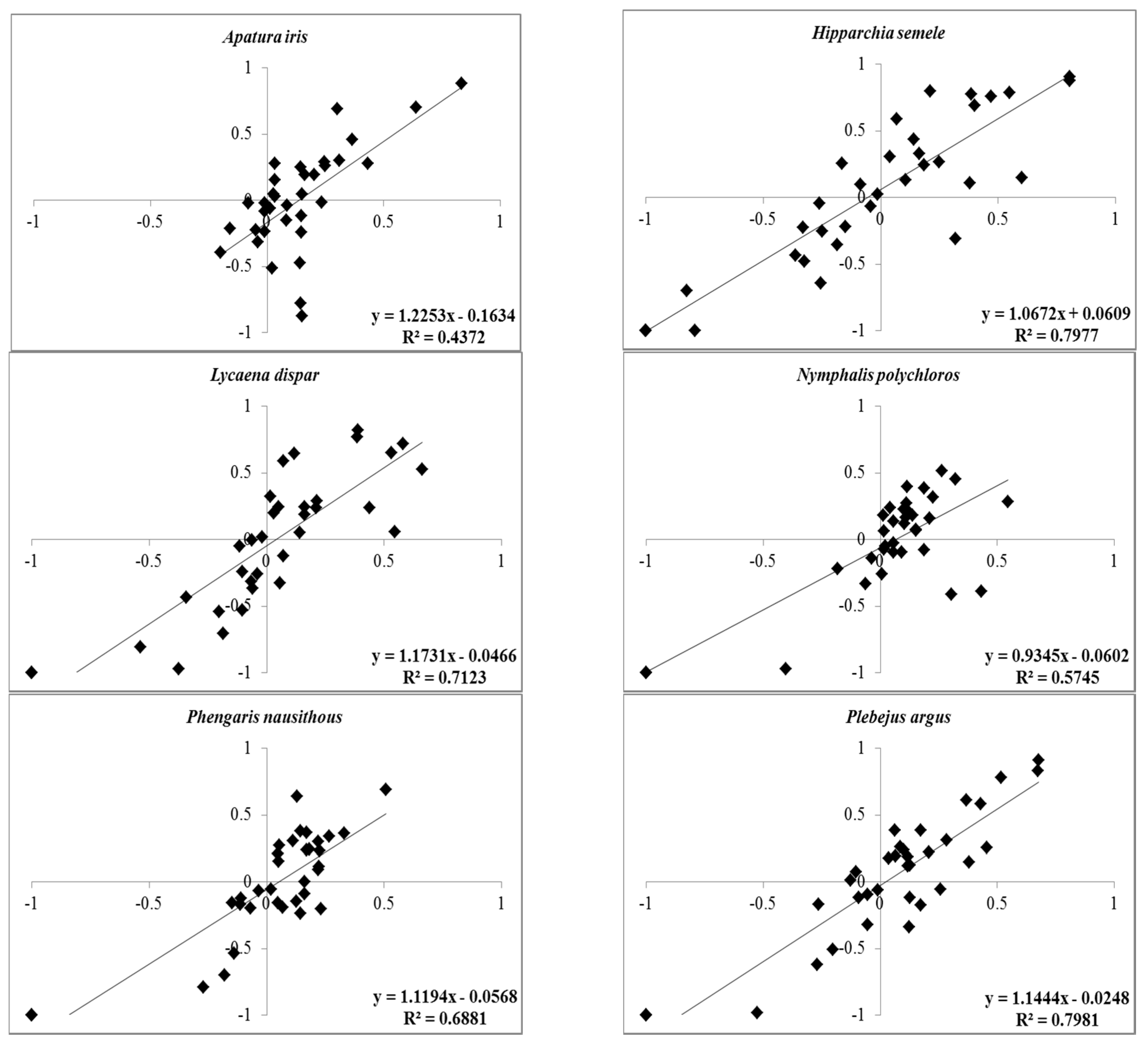
3.1. Relationship between Presence-Based Indices: Two Means for Calculating Ivlev’s Electivity Index

We found a strong positive relation between the values of IEIoccup based on number of occupied cells in land-cover classes, and IEIabund based on abundance of land cover classes within 1 km squares, for three out of six species: P. argus (R2 = 0.7981), H. semele (R2 = 0.7977), and L. dispar (R2 = 0.7123). A slightly weaker relation was found for P. nausithous (R2 = 0.6881) and clearly weaker ones for N. polychloros (R2 = 0.5745) and A. iris (R2 = 0.4372). Results are here presented in the form of a regression instead of Pearson’s correlation in order to assess also the slope of the relationship: Deviation of the regression slope between the two indices from 1, indicating a bias in the IEI values, was observed especially for A. iris and L. dispar (slope = 1.23 and 1.17, respectively), primarily due to a few outliers occurring for some unfavorable habitats (Figure 1).

3.2. Effect of Area on Ivlev’s Electivity Indices

In an assessment of the potential effect of land-cover area (abundance of a given land-cover) on IEI values, we found no such effect for three of the species. After removing two outliers, the effect was weak for both indices for H. semele (R2 = 0.2166 for IEIoccup and R2 =0.1863 for IEIabund), and also weak for P. nausithous (R2 = 0.1343) and P. argus (R2 = 0.1128) for IEIabund (Table 1). Results, however, were only marginally significant (0.05 < p < 0.1 prior to Bonferroni correction). Main outliers, namely highly abundant land-covers, were grasslands (land-cover code: 41) and arable fields (land-cover code: 81), but also coniferous forests (72) for H. semele and A. iris, and scree slopes for A. iris (52).

3.3. Expert Opinion Habitat Suitability Variance Analysis

We found a strong negative relation for H. semele (R2 = 0.848) between the average expert ranking of habitat suitability and the variance between answers, a medium strength of relation for N. polychloros (R2 = 0.4998), P. nausithous (R2 = 0.476), and L. dispar (R2 = 0.4087), but a substantially lower value for P. argus (R2 = 0.267) and A. iris (R2 = 0.202). This negative relation indicates that experts tended to agree about the less suitable habitats, but provided highly diverse answers with respect to potentially suitable habitats, especially for H. semele.

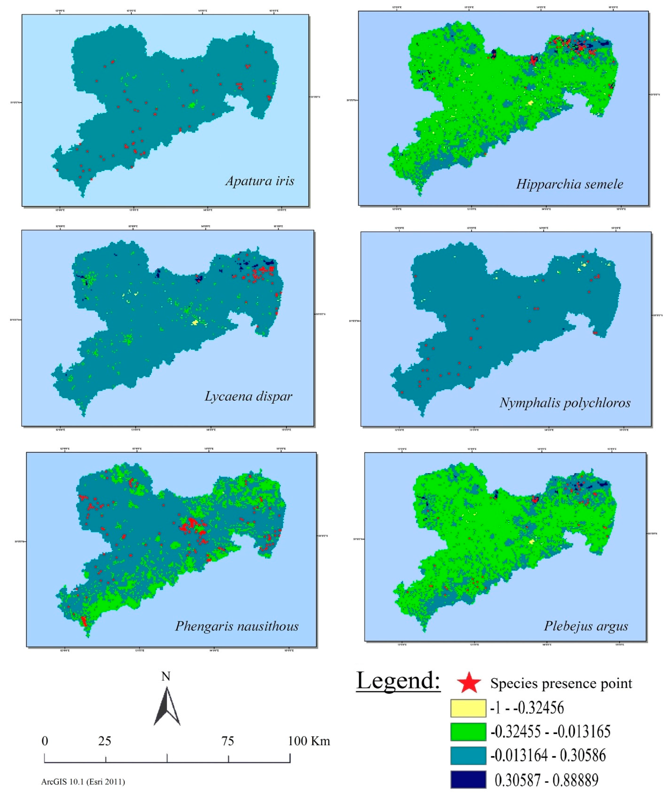
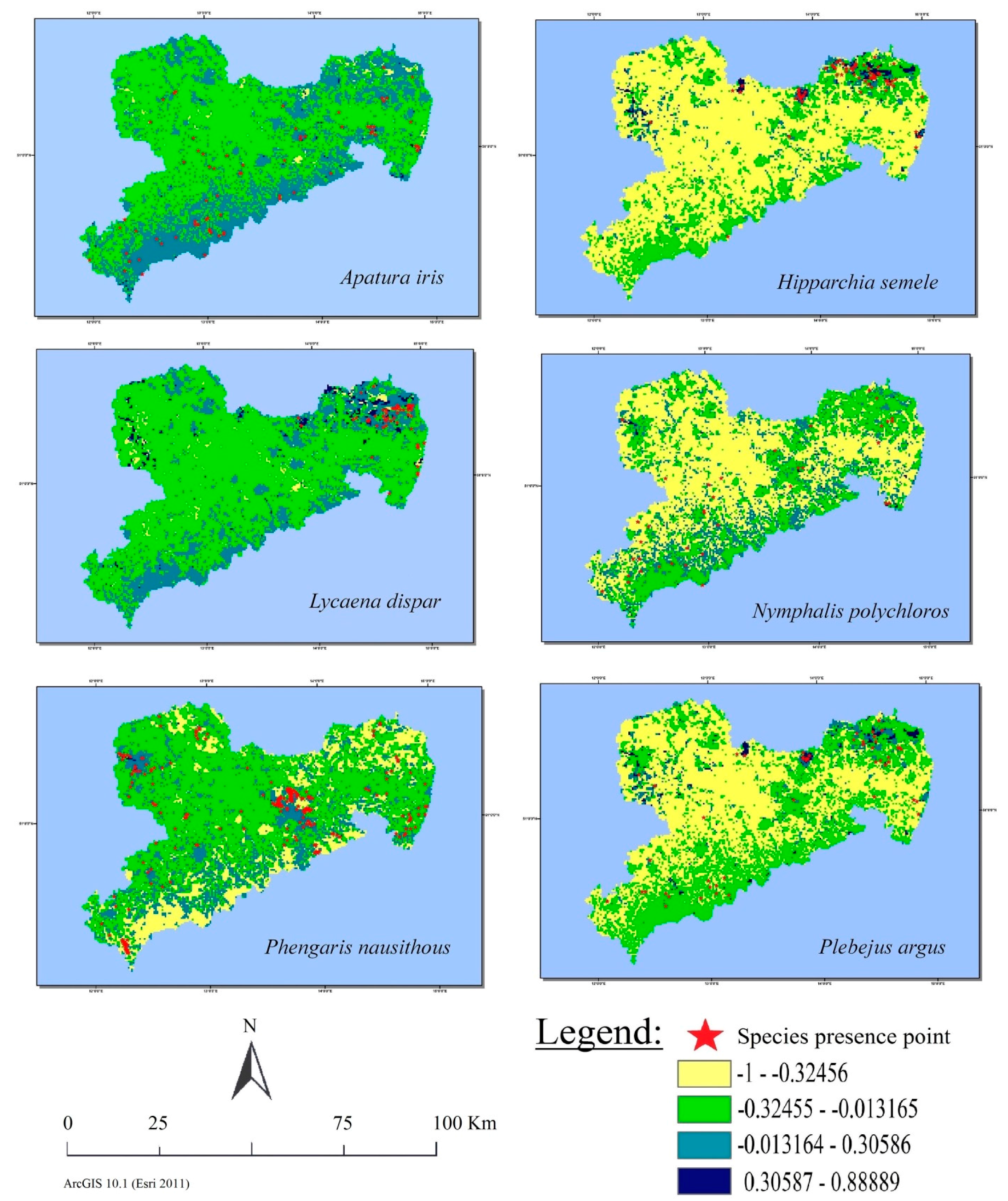
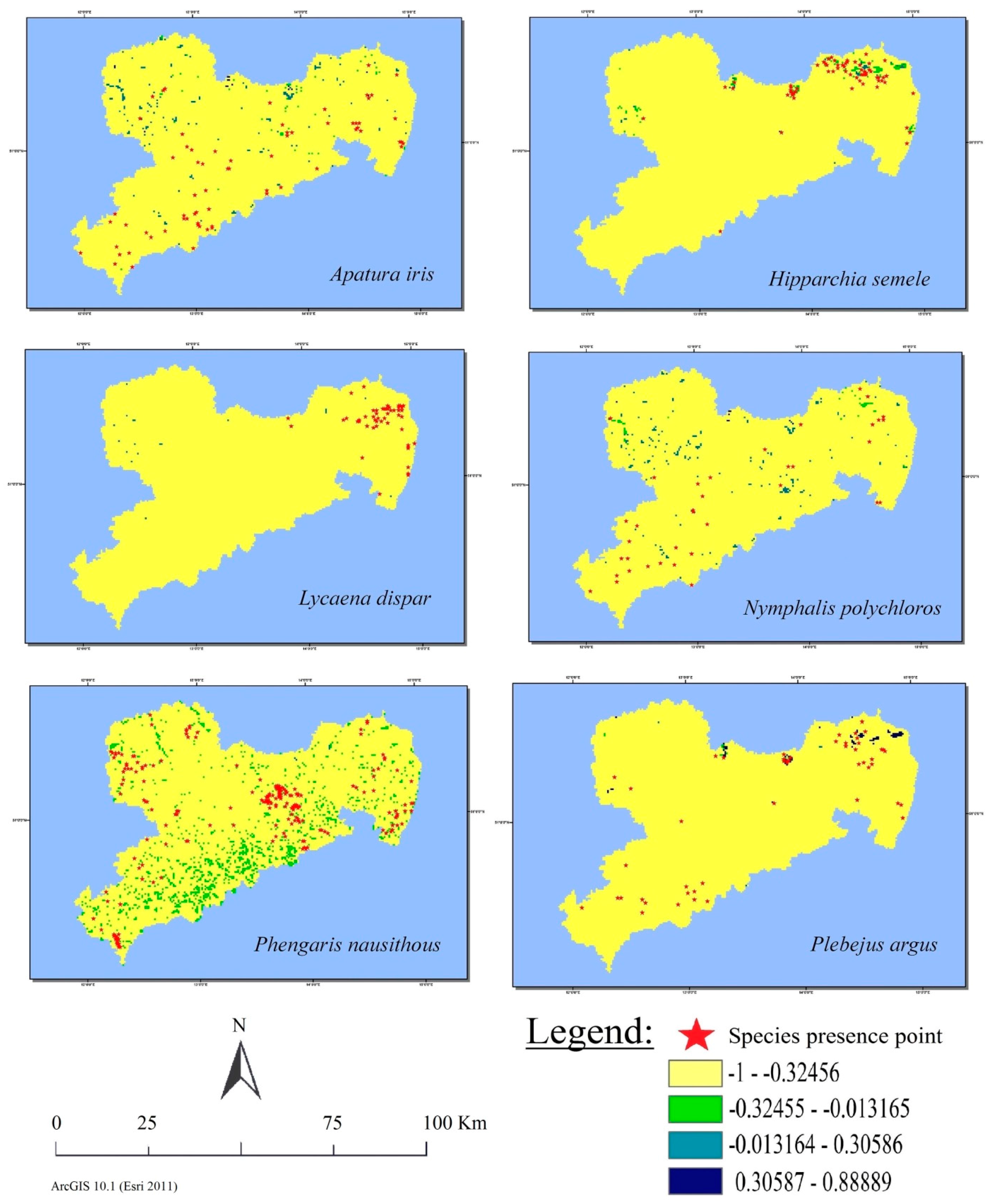
3.4. Visual Analysis of Land Cover Class Suitability Maps

Land cover maps produced using IEIoccup values identified distinctive geographical patterns of preference for three of the species (Figure 2). By contrast, maps produced using IEIabund yielded distinctive spatial patterns for all six species (Figure 3). More specifically, the southern and north-eastern regions of the State of Saxony were predominantly the most preferred for species, excluding P. nausithous, whereas IEIoccup maps did not show a distinctive area of high preference for the species A. iris, L. dispar and N. polychloros. However, IEIabund maps showed fine patterns of suitable and unsuitable areas in comparison to IEIoccup for all 6 species (Figure 2 and Figure 3).
The preference map for P. nausithous clearly differed from the maps of the other species (Figure 2 and Figure 3): Most of the preferred areas were located in a more scattered manner from IEIabund maps, mainly in the centre and north-western parts of the study area (corresponding to flatland areas dominated by high coverage of agricultural land-covers). According to the IEIoccup maps, the preferred areas were more stretched in the same directions as in IEIabund. Further, for P. nausithous, presence points were distributed near preferred areas as identified both by IEIoccup and IEIabund values. By contrast, for A. iris and N. polychloros, preference maps from IEIoccup were relatively homogenous and indicated most of the State of Saxony as suitable for the species, whereas for both species IEIabund produced a map with distinct geographic differentiation between suitable and unsuitable regions. Yet note that observation points for the two species were indeed scattered throughout the study area (red stars in Figure 2 and Figure 3).
After conversion of the average expert opinion into suitability maps, the only relatively clear geographic patterns were for H. semele and P. argus, matching with most of the presence points in north-east Saxony (Figure 4). For the other four species, presence points occurred also in less suitable areas (red stars in Figure 4). All six maps indicated far lower suitability when compared to the maps produced by IEI (compare Figure 4 with Figure 2 and Figure 3). This is due to an overall lower scoring of the suitability given by experts.

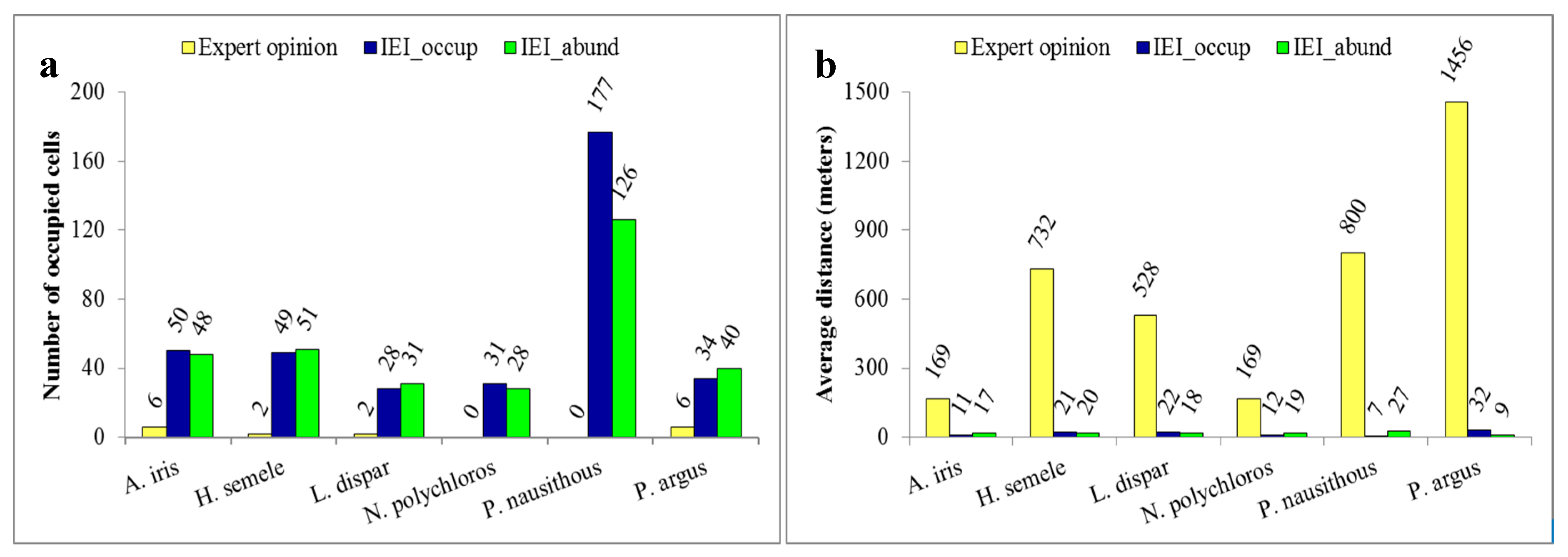
3.5. Spatial Relation between Observations and Suitable Habitats

The number of cells with preferred habitat, which also hosted observation points, was much higher for the maps produced from Ivlev’s electivity indices than for the maps produced from expert opinions, for all six species. The number of occupancy cells included based on IEIoccup was much greater than IEIabund for P. nausithous, but otherwise, it was nearly equal for the other five species (Figure 5a).
The average distance between presence points and nearest polygons of preferred suitable habitat was by far larger within the maps produced from expert opinions when compared to those originating from IEI values, for all six species (Figure 5b). While the average values were as low as seven meters for P. nausithous based on IEIoccup values, they reached 732 meters (H. semele), 800 meters (P. nausithous) and even 1456 meters on average for expert opinions, with poorest results for P. argus (Figure 5b).

3.6. Outcomes of Evaluation of the Results by Experts

While performance criteria listed above may seem to indicate the presence-based results (IEI) as better than the expert evaluation, communication with the original experts and additional independent ones indicated otherwise. With regards to mismatches (i.e., IEI indicating very high preference and experts suggesting very low suitability, or vice versa), some evaluators were of the opinion that in most cases the experts performed better. For instance, mismatches for the species A. iris, L. dispar and N. polychloros were explained by the experts as emerging from too high IEI for habitats, such as water bodies, which are clearly unsuitable. Further, scree slopes and bedrocks received low IEIoccup values compared to expert opinions for H. semele, and the experts identified this habitat as clearly suitable (See Appendix B & Appendix C for a list of all cases of match and mismatch). Experts were further of the opinion that the habitat preferences produced by IEI are incorrect, as all six species have a much broader distribution across Europe and occur across most of the State of Saxony. Thus the experts considered the spatial pattern obtained by the presence-based analysis as incorrect.

3.7. Land Covers Class Permeability versus Suitability

We found no relation between the average expert opinion on permeability and the IEI-based value of habitat preference (Table 2). However, there was a medium to high correlation between the expert ranking of suitability and permeability for some species, with particularly high values for H. semele, L. dispar and P. nausithous. Low correlation was obtained for N. polychloros.

4. Discussion

4.1. Empirical Presence Data versus Expert Opinions for Habitat Suitability

We used different approaches in this study to compare empirical presence data and expert opinions about habitat suitability. At first sight, IEI yield more informative maps and suitability information than expert opinions for all six butterfly species. The habitat suitability preference maps for all six species based on expert opinions did not indicate any spatial differentiation across the topographical gradient (and land-cover differences) in Saxony, with the exception of Phengaris nausithous (Figure 4). Secondly, expert-based maps did not spatially match the observed localities (Figure 5). Finally, expert evaluations varied broadly between experts with hardly any clear patterns regarding habitat suitability. These results seem to concur with previous studies, suggesting that empirical data and statistical approaches provide better results than expert-based ones [36,56].
On the other hand, when we communicated with experts, mismatches between expert opinions and IEI-based suitability evaluations were explained by the experts as originating from wrong evaluations by the presence-based analysis (Appendix B & Appendix C). This outcome demonstrates that there is lot of in-field experience of the experts, which clearly extends beyond what presence-data analysis can reach and can serve in adding or removing land-cover types that may be otherwise falsely classified. Furthermore, local experts wished to clarify that the species have a much broader distribution than the state of Saxony, and therefore should not show a strong spatial suitability signature. Thus, our results also support criticism of habitat indices with regard to their mechanistic approach and lack of scientific precision [54,57,58].
At small scales, precision is another issue to consider and could be relatively easily assessed by visiting field sites. However, when working at regional or larger scales it is not possible to verify the given information over the whole region and we thus depend on large datasets on land cover and species distribution [6,59,60,61]. A visual inspection of the detailed raster when compared to the 1 km2 maps indicated that the positions of presence-points (red stars), as they were set to a single point within 1 km2 grid cells, likely do not reflect the exact habitat in which the species was originally observed, and in highly diverse landscape mosaics, they are actually unlikely to do so. In other words, the presences may actually fall into habitats that are of lower suitability because of small nearby patches of high suitability and thus the statistical model is incorrectly assigning high suitability values for more abundant habitat types, while biasing against small-scale habitats. Notably, most of the mismatches occurred for smaller-scale habitat types. Additionally, some presence records seem to be in unusual habitats because of migration events. For example, Reinhardt et al. (2007) explained the single record of Hipparchia semele in the upper regions of the Ore Mountains (Erzgebirge) by a single migration event from Bohemia [62]. Further, elevation has not been considered in preparing the IEI-maps. Potential habitats in the mountains, which were considered as suitable, may in fact be unsuitable because of the climatic niche of the assessed species (e.g., Lycaena dispar), and therefore, spatial gradients need to be re-inspected to consider more than just land cover. Finally, the suitability of rare habitat types is very difficult to evaluate using presence data, and hence these should be taken with caution. Experts may be better than statistical models to identify such discrepancies.
A crucial point regarding expert evaluations is that all experts expressed their opinions based on broad in-field knowledge of the six species and the biological (habitat) requirements of these—which are not restricted to Saxony, but spans over all of Central Europe and many years of observations. While habitats that are potentially suitable for an individual species may not be inhabited e.g., due to climatic restrictions or other limiting factors that experts may not have considered, e.g., specific management or land-cover patterns in Saxony. For instance, Lycaena dispar could have a much broader range of occurrence in Saxony since damp meadows with ample of docks (especially Rumex crispus and R. obtusifolius; two common larval food plants) are very abundant in Central Europe, but the species only very recently seemed to have expanded in Saxony, which might be linked to climate change [63].
Further sources of error or biases in evaluations are likely to occur due to the definition of land-cover types or because it is not necessary for insects to have a large amount of habitat (scale of study), but rather the right quality (plant species as food for monophagous insect larvae) or management. Also, the mobility of a species can affect suitability evaluations by both experts and statistical models. For instance, Nymphalis polychloros is a very mobile species and can often be observed in habitats that do not appear suitable. While observers are likely to record such observations, experts can probably distinguish them as records out of the habitat (namely, dispersal), but such evaluations are usually not recorded in large-scale databases and standardized abundance data that could identify such records are usually lacking.
Land-cover classification is another source of error in analyses based on presence-data: in this study, for instance, land-cover type class 41 (cultivated grasslands) comprise three different types, of which two can serve as excellent habitats for butterflies but the third, defined as intensive grassland, likely is hostile to most species. As these three classes are difficult to distinguish on aerial photos, they are clustered into one habitat code, but this likely affects both expert judgement and the outcomes of presence-data analysis. Finally, expert judgments may be inaccurate because of misunderstandings of the habitat classification. How habitat codes relate to a certain habitat class may be vague although perhaps in German it is all much clearer [36], and may also be sensitive to the scale of perception: open woodland, at a smaller scale, is in fact a mix of two habitats, woods and grasslands. Apart from this, the terms habitat suitability and permeability may themselves be confusing for experts. The quality of expert opinion based analysis could probably be enhanced by adding more experts, especially those who are well acquainted with different parts of the assessed region, but a risk remains that the variability among answers may remain unless these are decided in an interactive or iterative process, e.g., through a set of meetings with all experts.
All in all, we do not regard one approach as superior to the other, but the combination and interaction between the two as an improved route to enhance apprehension of species needs in a way that makes more effective use of data. For instance, the spatial structuring of habitat suitability across Saxony may still reveal more refined segregation that would not have been possible to identify otherwise, while errors in the presence-based evaluation could not have been revealed without the feedback from experts.

4.2. Landscape Permeability

Evaluations of landscape permeability enable us to learn about another potentially important relation between habitat structure and “suitability”. More specifically, the permeability values provided by experts seem to be related to habitat structure, e.g., open crops received high permeability for grassland species. However, the relation between seeming structure and suitability has recently been questioned [64]. Exactly for this reason, results are particularly important for cases where low correlation was found between the permeability and suitability evaluations provided by experts. This was the case especially for N. polychloros and to a lesser extent A. iris. These two species occur in heterogeneous habitats and especially habitat edges (between forest and open habitats). For these species, quite intuitively, both open habitats and forest should be permeable, but presence-based information is very unlikely to reveal any information on this aspect. On the other hand, grassland and open-habitat species, including H. semele, which often occurs in open habitats within forests, obtained low permeability values for forests. In this case, it seems that permeability was assigned by the experts as being associated with the structure of the species prime habitat. This, in fact, may not necessarily be true. Information on permeability from independent sources, however, is rare. Hovestadt et al. (2011) observed high dispersal rates of Phengaris nausithous in habitat patches that were frequently disturbed by mowing [32], while Nowicki et al. (2014) had recorded nearly no movements in the same species in patches under very slow succession for several years [65]. Sufficient empirical information regarding permeability for all species was not available to compare it with expert opinions.
There are nevertheless potential advantages for an expert evaluation separating suitability from permeability. First, by asking experts to report separately on suitability and permeability, one already enhances awareness to the difference between the two parameters. Secondly, one gains a better mechanistic answer to the question where species may occur, and whether such observations represent occurrence in reproductive habitats or movement through otherwise hostile (dispersal) environment. Such information cannot be obtained from presence data. Furthermore, since observers tend to report on unique observations, there is a plausible chance that presence data based on sporadic observations indeed includes cases of movement through non-reproductive habitats. Such observations, that would bias suitability values, can be rectified by asking experts to make a clear distinction. While it is impossible in this study to evaluate whether the estimations made by experts are correct, or to use them for rectifying erroneous suitability information, they at least provide a template for hypothesis testing, as well as means to separate habitat suitability from permeability for those species where seemingly such association is clearly wrong [66].

5. Conclusions

In this study, empirical presence data yielded very different habitat suitability values and maps than expert opinions. Our results suggest that statistical models based on empirical presence data need to be scrutinized against expert opinions that are well founded on high familiarity with the species and area of concern. Together, knowledge can be maximized regarding habitat suitability. Further, a clear understanding about both suitability and permeability can help in developing sensible conservation policies that could enhance our capacity to achieve species persistence in light of ample environmental risks.
We would suggest rectifying presence-based maps with expert opinions where the latter clearly indicate the suitability evaluation by presence data might be wrong (mismatches between expert opinions and IEI). Further, these results can be tested against independent data, which unfortunately was unavailable in this study but is becoming increasingly available, e.g., through the German Butterfly Monitoring Scheme (TMD) [67]. Additionally, expert opinions on permeability can be used as an additional input for conservation planning tools, such as the software Zonation (University of Helsinki, Helsinki, Finland) [68]. In the future, we intend to compare the maps produced by such tools when considering land cover class preferences only (based on experts or presence-data), as compared to when considering also permeability and hence potential connectivity between natural habitats. Thereby, we can advance the inclusion of functional connectivity in conservation planning.

Acknowledgments

We thank the experts who shared their opinions and participated in valuable discussions: Gerd Kuna, Hans Moser, Jürgen Hensle, Stefan Brunzel, Elisabeth Kühn, Martin Wiemers and Piotr Nowicki. Presence data originate from Entomofauna Saxonica, kindly provided by Rolf Reinhardt. Land-cover data of Saxony was provided by Saxon State Agency for Environment, Agriculture and Geology (LfULG). We wish to express our gratitude to members of the Department of Conservation Biology at the UFZ and especially the members of the working group “Population Ecology and Landscape Structure” for valuable discussions. The work was enabled by an Erasmus fellowship to Muhammad Arfan by Lund University. Reinhard Klenke was funded by SCALES (contract 226852).

Author Contributions

Muhammad Arfan analyzed data and prepared the manuscript. Bianca Bauch, Guy Pe’er and Reinhard Klenke planned the experiment. Bianca Bauch collected the data. Guy Pe’er, Josef Settele, Klaus Henle and Reinhard Klenke helped in drafting the manuscript and interpretation of the results. All authors contributed to revisions and completion of the manuscript.

Conflicts of Interest

We have already mentioned funding sources in acknowledgment section; no other relationships or activities that could appear to have influenced the submitted work.

Appendix A. Land-Cover Types and Habitat Types (BTLNK) of Saxony Vector Map (Lfulg 2008) [51]

BTLNKOriginal German Land Cover DescriptionEnglish Translation of Land Cover Class
21Flieβgewässerstreaming water
23Stillgewässerstanding waterbody
24Gewässerbegleitende Vegetationriparian vegetation
25Bauwerke an Gewässernconstruction at waterbody
31Hochmoor, Zwischenmoorraised bogs and transitional mires
32Niedermoor, Sumpffens and swamp land
41Wirtschaftsgrünlandgrasslands and (managed) meadows
42Ruderalflur, Staudenflurruderal and herbaceous vegetation
51Anstehender Felsbedrock
52Blockschutthaldenscree slopes
53größere Lesesteinhaufen und offene Steinrückenlarge clearance cairns and open rocks
54Offene Flächenopen areas
55Zwergstrauchheiden und Borstgrasrasendwarf shrub heath and Nardus grassland
56Magerrasen trockener Standortedry abandoned grasslands
61Feldgehölz, Baumgruppe 100 m2–1 hagroup of trees 100 m2–1 ha
66Gebüschscrubland
67neu ab 2005: Streuobstwiesemeadow with fruit trees
70Wiederaufforstungreforestation
71Laubbaumart (Reinbestand)broad leaved forest
72Nadelbaumart (Reinbestand)coniferous forest
73Laub-Nadel-Mischwaldmixed forest (broad-leaved-coniferous)
74Nadel-Laub-Mischwaldmixed forest (coniferous-broad-leaved)
75Laubmischwaldmixed forest (broad-leaved)
76Nadelmischwaldmixed forest (coniferous)
77Feuchtwälder (Moorwald siehe 31300)mesic forest
78Waldrandbereiche/Vorwälderforest edges, pioneer forest
79Erstaufforstungafforestation
81Ackerarable land
82Sonderkulturenspecialised crop
91Wohngebietresidential area
92Mischgebietmixed area
93Gewerbegebietindustrial area
94Grün- und Freiflächengreen spaces
95Verkehrsflächentraffic area
96Anthropogen genutzte Sonderflächenhuman used special areas

Appendix B. Habitat Suitability Analysis Based on Expert Opinions versus IEIoccup for Six Butterfly Species

Species NameBTLNKBTLNK-DefinationStatusIEIoccupExpert
Apatura iris75deciduous mixed forestsMatchhighhigh
78forest edges, pioneer forestMatchhighhigh
67meadow with fruit treesMatchlowlow
82specialized cropMatchlowlow
25construction at water bodyMismatchhighlow
52scree slopesMismatchhighlow
Hipparchia semele56dry abandoned grasslandsMatchhighhigh
54open areasMatchhighhigh
67meadow with fruit treesMatchlowlow
82specialized cropMatchlowlow
31raised bogs and transitional miresMismatchhighlow
32fens and swamp landMismatchhighlow
51bedrockMismatchlowhigh
52scree slopesMismatchlowhigh
Lycaena dispar24riparian vegetationMatchhighhigh
32fens and swamp landMatchhighhigh
52scree slopesMatchlowlow
53large clearance cairns and open rocksMatchlowlow
25construction at water bodyMismatchhighlow
56dry abandoned grasslandsMismatchhighlow
Nymphalis polychloros78forest edges, pioneer forestMatchhighhigh
75deciduous mixed forestsMatchhighhigh
52scree slopesMatchlowlow
31raised bogs and transitional miresMatchlowlow
25construction at water bodyMismatchhighlow
51bedrockMismatchhighlow
Phengaris nausithous24riparian vegetationMatchhighhigh
32fens and swamp landMatchhighhigh
31raised bogs and transitional miresMatchlowlow
52scree slopesMatchlowlow
82specialized cropMismatchhighlow
Plebejus argus55dwarf shrub heath and Nardus grasslandMatchhighhigh
56dry abandoned grasslandsMatchhighhigh
51bedrockMatchlowlow
52scree slopesMatchlowlow
32fens and swamp landMismatchhighlow
77mesic forestMismatchhighlow

Appendix C. Habitat Suitability Analysis Based on Expert Opinions versus IEIabund for Six Butterfly Species

Species NameBTLNKBTLNK-DefinationStatusIEIabundExpert
Apatura iris51bedrockMatchlowlow
55dwarf shrub heath Matchlowlow
25construction at water bodyMismatchhighlow
52scree slopesMismatchhighlow
77mesic forestMismatchlowhigh
78forest edges, pioneer forestMismatchlowhigh
Hipparchia semele55dwarf shrub heath Matchhighhigh
56dry abandoned grasslandsMatchhighhigh
67meadow with fruit treesMatchlowlow
81arable landMatchlowlow
32fens and swamp landMismatchhighlow
77mesic forestMismatchhighlow
51bedrockMismatchlowhigh
52scree slopesMismatchlowhigh
Lycaena dispar24riparian vegetationMatchhighhigh
32fens and swamp landMatchhighhigh
52scree slopesMatchlowlow
53large clearance and open rocksMatchlowlow
55dwarf shrub heath Mismatchhighlow
77mesic forestMismatchhighlow
Nymphalis polychloros75mixed forest (broad-leaved)Matchhighhigh
78forest edges, pioneer forestMatchhighhigh
31raised bogs and transitional miresMatchlowlow
52scree slopesMatchlowlow
24riparian vegetationMismatchhighlow
76mixed forest (coniferous)Mismatchhighlow
67meadow with fruit treesMismatchlowhigh
82specialized cropMismatchlowhigh
Phengaris nausithous51bedrockMatchlowlow
52scree slopesMatchlowlow
82specialized cropMismatchhighlow
Plebejus argus55dwarf shrub heath Matchhighhigh
56dry abandoned grasslandsMatchhighhigh
51bedrockMatchlowlow
52scree slopesMatchlowlow
32fens and swamp landMismatchhighlow
77mesic forestMismatchhighlow

References

  1. Keller, B.D.; Gleason, D.F.; McLeod, E.; Woodley, C.M.; Airamé, S.; Causey, B.D.; Friedlander, A.M.; Grober-Dunsmore, R.; Johnson, J.E.; Miller, S.L.; et al. Climate change, coral reef ecosystems, and management options for marine protected areas. Environ. Manag. 2009, 44, 1069–1088. [Google Scholar] [CrossRef] [PubMed]
  2. Convention on Biological Diversity. Available online: http://www.cbd.int/decision/cop/?id=12268 (accessed on 7 December 2016).
  3. Margules, C.R.; Pressey, R.L. Systematic conservation planning. Nature 2000, 405, 243–253. [Google Scholar] [CrossRef] [PubMed]
  4. Kingsland, S.E. Creating a science of nature reserve design: Perspectives from history. Environ. Model. Assess. 2002, 7, 61–69. [Google Scholar] [CrossRef]
  5. Soberón, J.; Peterson, T. Biodiversity informatics: Managing and applying primary biodiversity data. Philos. Trans. R. Soc. Lond. B 2004, 359, 689–698. [Google Scholar] [CrossRef] [PubMed]
  6. Guralnick, R.P.; Hill, A.W.; Lane, M. Towards a collaborative, global infrastructure for biodiversity assessment. Ecol. Lett. 2007, 10, 663–672. [Google Scholar] [CrossRef] [PubMed]
  7. Hortal, J.; Lobo, J.M.; Jimenez-Valverde, A. Limitations of biodiversity databases: Case study on seed-plant diversity in Tenerife, Canary Islands. Conserv. Biol. 2007, 21, 853–863. [Google Scholar] [CrossRef] [PubMed]
  8. Gibson, L.A.; Wilson, B.A.; Cahill, D.M.; Hill, J. Spatial prediction of rufous bristlebird habitat in a coastal heathland: A GIS-based approach. J. Appl. Ecol. 2004, 41, 213–223. [Google Scholar] [CrossRef]
  9. Posillico, M.; Meriggi, A.; Pagnin, E.; Lovari, S.; Russo, L. A habitat model for brown bear conservation and land use planning in the central Apennines. Biol. Conserv. 2004, 118, 141–150. [Google Scholar] [CrossRef]
  10. Wintle, B.A.; Elith, J.; Potts, J.M. Fauna habitat modelling and mapping: A review and case study in the Lower Hunter Central Coast region of NSW. Austral Ecol. 2005, 30, 719–738. [Google Scholar] [CrossRef]
  11. Lobo, J.M.; Lumaret, J.P.; JayRobert, P. Taxonomic databases as tools in spatial biodiversity research. Ann. Soc. Entomol. Fr. 1997, 33, 129–138. [Google Scholar]
  12. Hanski, I.; Gaggiotti, O.E. Ecology, Genetics and Evolution of Metapopulations; Academic Press: Burlington, VT, USA, 2004; pp. ix–xix. [Google Scholar]
  13. Myers, N.; Mittermeier, R.A.; Mittermeier, C.G.; da Fonseca, G.A.B.; Kent, J. Biodiversity hotspots for conservation priorities. Nature 2000, 403, 853–858. [Google Scholar] [CrossRef] [PubMed]
  14. Pullin, A.S.; Knight, T.M. Effectiveness in conservation practice: Pointers from medicine and public health. Conserv. Biol. 2001, 15, 50–54. [Google Scholar] [CrossRef]
  15. Guisan, A.; Thuiller, W. Predicting species distribution: Offering more than simple habitat models. Ecol. Lett. 2005, 8, 993–1009. [Google Scholar] [CrossRef]
  16. Elith, J.; Graham, C.H.; Anderson, R.P.; Dudík, M.; Ferrier, S.; Guisan, A.; Hijmans, R.J.; Huettmann, F.; Leathwick, J.R.; Lehmann, A.; et al. Novel methods improve prediction of species’ distributions from occurrence data. Ecography 2006, 29, 129–151. [Google Scholar] [CrossRef]
  17. Whigham, P.A. Induction of a marsupial density model using genetic programming and spatial relationships. Ecol. Model. 2000, 131, 299–317. [Google Scholar] [CrossRef]
  18. Hirzel, A.H.; Guisan, A. Which is the optimal sampling strategy for habitat suitability modelling? Ecol. Model. 2002, 157, 331–341. [Google Scholar] [CrossRef]
  19. Cawsey, E.M.; Austin, M.P.; Baker, B.L. Regional vegetation mapping in Australia: A case study in the practical use of statistical modeling. Biodivers. Conserv. 2002, 11, 2239–2274. [Google Scholar] [CrossRef]
  20. Graham, C.H.; Ferrier, S.; Huettman, F.; Moritz, C.; Peterson, A.T. New developments in museum based informatics and applications in biodiversity analysis. Trends Ecol. Evol. 2004, 19, 497–503. [Google Scholar] [CrossRef] [PubMed]
  21. Huettmann, F. Databases and science-based management in the context of wildlife and habitat: Towards a certified ISO standard for objective decision-making for the global community by using the internet. J. Wildl. Manag. 2005, 69, 466–472. [Google Scholar] [CrossRef]
  22. Soberón, J.; Peterson, A.T. Interpretation of models of fundamental ecological niches and species distributional areas. Biodivers. Inform. 2005, 2, 1–10. [Google Scholar] [CrossRef]
  23. Noss, R.F.; Cooperrider, A.Y. Saving Nature’s Legacy: Protecting and Restoring Biodiversity; Island Press: Washington, DC, USA, 1994; pp. 1–416. [Google Scholar]
  24. Prevedello, J.A.; Vieira, M.V. Does the type of matrix matter? A quantitative review of the evidence. Biodivers. Conserv. 2010, 19, 1205–1223. [Google Scholar] [CrossRef]
  25. Hall, L.S.; Krausman, P.R.; Morrison, M.L. The habitat concept and a plea for standard terminology. Wildl. Soc. B 1997, 25, 173–182. [Google Scholar]
  26. Dennis, R.L.H.; Shreeve, T.G.; Dyck, H.V. Habitats and resources: The need for a resource-based definition to conserve butterflies. Biodivers. Conserv. 2006, 15, 1943–1966. [Google Scholar] [CrossRef]
  27. Vanreusel, W.; Dyck, H.V. When functional habitat does not match vegetation types: A resource-based approach to map butterfly habitat. Biol. Conserv. 2007, 135, 202–211. [Google Scholar] [CrossRef]
  28. Meiklejohn, K.; Ament, R.; Tabor, G. Habitat Corridors & Landscape Connectivity: Clarifying the Terminology; Center for Large Landscape Conservation: Bozeman, MT, USA, 2010; pp. i–ix. [Google Scholar]
  29. Lindenmayor, D.; Fischer, J. Habitat Fragmentation and Landscape Change: An Ecological and Conservation Synthesis; Island Press: Washington, DC, USA, 2006; pp. 1–352. [Google Scholar]
  30. Heller, N.E.; Zavaleta, E.S. Biodiversity management in the face of climate change: A review of 22 years of recommendations. Biol. Conserv. 2009, 142, 14–32. [Google Scholar] [CrossRef]
  31. Krosby, M.; Tewksbury, J.; Haddad, N.M.; Hoekstra, J. Ecological connectivity for a changing climate. Conserv. Biol. 2010, 24, 1686–1689. [Google Scholar] [CrossRef] [PubMed]
  32. Hovestadt, T.; Binzenhöfer, B.; Nowicki, P.; Settele, J. Do all inter-patch movements represent dispersal? A mixed kernel study of butterfly mobility in fragmented landscapes. J. Anim. Ecol. 2011, 80, 1070–1077. [Google Scholar] [CrossRef] [PubMed]
  33. Drew, C.A.; Collazo, J.A. Expert knowledge as a foundation for the management of secretive species and their habitat (Chapter 5). In Expert Knowledge and Its Application in Landscape Ecology; Perera, A.H., Drew, C.A., Johnson, C.J., Eds.; Springer: New York, NY, USA, 2011; pp. 87–107. [Google Scholar]
  34. Drew, C.A.; Perera, A.H. Expert knowledge as a basis for landscape ecological predictive models (Chapter 12). In Predictive Species and Habitat Modeling in Landscape Ecology: Concepts and Applications; Drew, C.A., Wiersma, Y.F., Huettmann, F., Eds.; Springer: New York, NY, USA, 2011; pp. 229–248. [Google Scholar]
  35. Clevenger, A.P.; Wierzchowski, J.; Chruszcz, B.; Gunson, K. GIS-generated, expert-based models for identifying wildlife habitat linkages and planning mitigation passages. Conserv. Biol. 2002, 16, 503–514. [Google Scholar] [CrossRef]
  36. Johnson, C.J.; Gillingham, M.P. Mapping uncertainty: Sensitivity of wildlife habitat ratings to Expert opinion. J. Appl. Ecol. 2004, 41, 1032–1041. [Google Scholar] [CrossRef]
  37. Choy, S.L.; O’Leary, R.; Mengersen, K. Elicitation by design for ecology: Using expert opinion to inform priors for Bayesian statistical models. Ecology 2009, 90, 265–277. [Google Scholar] [CrossRef] [PubMed]
  38. Schlossberg, S.; King, D.I. Modeling animal habitats based on cover types: A critical review. Environ. Manag. 2009, 43, 609–618. [Google Scholar] [CrossRef] [PubMed]
  39. Johnson, C.J.; Hurley, M.; Rapaport, E.; Pullinger, M. Using expert knowledge effectively: Lessons from species distribution models for wildlife conservation and management (Chapter 8). In Expert Knowledge and Its Application in Landscape Ecology; Perera, A.H., Drew, C.A., Johnson, C.J., Eds.; Springer: New York, NY, USA, 2012; pp. 153–171. [Google Scholar]
  40. Thomas, J.A.; Telfer, M.G.; Roy, D.B.; Preston, C.D.; Greenwood, J.J.; Asher, J.; Fox, R.; Clarke, R.T.; Lawton, J.H. Comparative losses of British butterflies, birds and plants and the global extinction crisis. Science 2004, 303, 1879–1881. [Google Scholar] [CrossRef] [PubMed]
  41. Thomas, J.A. Monitoring change in the abundance and distribution of insects using butterflies and other indicator groups. Philos. Trans. R. Soc. Lond. B 2005, 360, 339–357. [Google Scholar] [CrossRef] [PubMed]
  42. Pe’er, G.; Settele, J. Butterflies in and for conservation: Trends and Prospects. Isr. J. Ecol. Evol. 2008, 54, 7–17. [Google Scholar] [CrossRef]
  43. Van Swaay, C.; Van Strien, A.; Aghababyan, K.; Astrom, S.; Botham, M.; Brereton, T.; Chambers, P.; Collins, S.; Domenech Ferre, M.; Escobes, R.; et al. The European Butterfly Indicator for Grassland Species: 1990–2013; De Vlinderstichting: Wageningen, The Netherlands, 2015; pp. 1–39. [Google Scholar]
  44. Spänhoff, B.; Dimmer, R.; Friese, H.; Harnapp, S.; Herbst, F.; Jenemann, K.; Mickel, A.; Rohde, S.; Schönherr, M.; Ziegler, K.; et al. Ecological status of rivers and streams in Saxony (Germany) according to the water framework directive and prospects of improvement. Water 2012, 4, 887–904. [Google Scholar] [CrossRef]
  45. Renner, M.; Bernhofer, C. Long term variability of the annual hydrological regime and sensitivity to temperature phase shifts in Saxony/Germany. Hydrol. Earth Syst. Sci. 2011, 15, 1819–1833. [Google Scholar] [CrossRef]
  46. Bastian, O. Landscape classification in Saxony (Germany)—A tool for holistic regional planning. Landsc. Urban Plan. 2010, 50, 145–155. [Google Scholar] [CrossRef]
  47. Gimenez-Dixon, M. Lycaena dispar. IUCN 2012. IUCN Red List of Threatened Species; Version 2012.2. Available online: www.iucnredlist.org (accessed on 8 July 2015).
  48. World Conservation Monitoring Centre. Phengaris nausithous. IUCN 2012. IUCN Red List of Threatened Species; Version 2012.2. 1996. Available online: www.iucnredlist.org (accessed on 13 December 2013).
  49. Van Swaay, C.; Wynhoff, I.; Verovnik, R.; Wiemers, M.; López Munguira, M.; Maes, D.; Sasic, M.; Verstrael, T.; Warren, M.; Settele, J. Hipparchia semele. IUCN 2012. IUCN Red List of Threatened Species; Version 2012.2. 2010. Available online: www.iucnredlist.org (accessed on 22 December 2013).
  50. Belgian Species List. Nymphalis polychloros (Linnaeus, 1758). Available online: http://www.species.be/en/3063 (accessed on 15 October 2015).
  51. LfULG. Biotope and Land Use Map of Saxony, Germany 2005. 2008. Available online: http://www.umwelt.sachsen.de/umwelt/natur/18615.htm (accessed on 11 April 2012).
  52. Ivlev, V.S. Experimental Ecology of the Feeding of Fishes; Yale University Press: New Haven, CT, USA, 1961; pp. 1–302. [Google Scholar]
  53. Aryal, A.; Raubenheimer, D.; Subedi, S.; Kattel, B. Spatial habitat overlap and habitat preference of Himalayan Musk Deer (Moschus chrysogaster) in Sagarmatha (Mt. Everest) national park, Nepal. J. Biol. Sci. 2010, 2, 217–225. [Google Scholar]
  54. Storch, I. On spatial resolution in habitat models: Can small-scale forest structure explain Capercaillie numbers? Conserv. Ecol. 2002, 6, 6. [Google Scholar] [CrossRef]
  55. ESRI. ArcGIS Desktop: Release 10; Environmental Systems Research Institute: Redlands, CA, USA, 2011. [Google Scholar]
  56. Pearce, J.L.; Cherry, K.; Drielsma, M.; Ferrier, S.; Whish, G. Incorporating expert opinion and fine-scale vegetation mapping into statistical models of faunal distribution. J. Appl. Ecol. 2001, 38, 412–424. [Google Scholar] [CrossRef]
  57. Brooks, R.P. Improving habitat suitability index models. Wildl. Soc. B 1997, 25, 163–167. [Google Scholar]
  58. Henle, K.; Potts, S.; Kunin, W.; Matsinos, Y.; Similä, J.; Pantis, J.; Grobelnik, V.; Penev, L.; Settele, J. Scaling in Ecology and Biodiversity Conservation; Pensoft Publishers: Sofia, Bulgaria, 2014; p. e1169. [Google Scholar]
  59. Edenius, L.; Elmberg, J. Landscape level effects of modern forestry on bird communities in North Swedish boreal forests. Landsc. Ecol. 1996, 11, 325–338. [Google Scholar] [CrossRef]
  60. Saab, V. Importance of spatial scale to habitat use by breeding birds in riparian forests: A hierarchical analysis. Ecol. Appl. 1999, 9, 135–151. [Google Scholar] [CrossRef]
  61. Graf, R.F.; Bollmann, K.; Suter, W.; Bugmann, H. The importance of spatial scale in habitat models: Capercaillie in the Swiss Alps. Landsc. Ecol. 2005, 20, 703–717. [Google Scholar] [CrossRef]
  62. Reinhardt, R.; Sbieschne, H.; Settele, J.; Fischer, U.; Fiedler, G. Tagfalter von Sachsen; Entomologische Nachrichten und Berichte: Dresden, Germany, 2007; pp. 1–695. [Google Scholar]
  63. Settele, J.; Kudrna, O.; Harpke, A.; Kühn, I.; van Swaay, C.; Verovnik, R.; Warren, M.; Wiemers, M.; Hanspach, J.; Hickler, T.; et al. Climatic Risk Atlas of European Butterflies. BioRisk 2008, 1, 1–710. [Google Scholar] [CrossRef]
  64. Pe’er, G.; Henle, K.; Dislich, C.; Frank, K. Breaking functional connectivity into components: A novel approach using an Individual-Based model, and first outcomes. PLoS ONE 2011, 6. [Google Scholar] [CrossRef]
  65. Nowicki, P.; Vrabec, V.; Binzenhofer, B.; Feil, J.; Zaksek, B.; Hovestadt, T.; Settele, J. Butterfly dispersal in inhospitable matrix: Rare, risky, but long-distance. Landsc. Ecol. 2014, 29, 401–412. [Google Scholar] [CrossRef]
  66. Dover, J.; Settele, J. The influences of landscape structure on butterfly distribution and movement: A review. J. Insect Conserv. 2009, 13, 3–27. [Google Scholar] [CrossRef]
  67. Kühn, E.; Feldmann, R.; Harpke, A.; Hirneisen, N.; Musche, M.; Leopold, P.; Settele, J. Getting the public involved into butterfly conservation—Lessons learned from a new monitoring scheme in Germany. Isr. J. Ecol. Evol. 2008, 54, 89–103. [Google Scholar] [CrossRef]
  68. Moilanen, A.; Kujala, H.; Leathwick, J. The Zonation framework and software for conservation prioritization. In Spatial Conservation Prioritization: Quantitative Methods and Computational Tools; Moilanen, A., Wilson, K.A., Possingham, H.P., Eds.; Oxford University Press: Oxford, UK, 2009; pp. 196–210. [Google Scholar]
Figure 1. Relationship between IEIoccup (X) and IEIabund (Y) in terms of habitat suitability of each land-cover types for the six species, based on presence data.
Environments 05 00036 g001
Figure 2. Maps of habitat preference based on IEIoccup for all six species (IEI values towards −1.0 indicate avoidance while +1.0 represents suitable).
Environments 05 00036 g002
Figure 3. Maps of habitat preference based on IEIabund for all six species (IEI values towards −1.0 indicate avoidance while +1.0 represents suitable).
Environments 05 00036 g003
Figure 4. Maps of average habitat suitability based on experts opinions for all six species (HS values towards −1.0 indicate avoidance while +1.0 represents suitable).
Environments 05 00036 g004
Figure 5. Spatial concurrence between observations and evaluations: (a) Number of occupied cells found in preferred suitable area based on IEI and experts opinions, and (b) average distance between the occupied cells and nearest suitable habitat.
Environments 05 00036 g005
Table 1. Effect of land-cover area (X) on Ivlev’s electivity indices (IEI) (Y) values for all butterfly species.
Species NameIndicesR2-Value *R2-Value **Equation ***
Apatura irisIEIoccup0.01330.025y = −1E− 08x + 0.1581
IEIabund0.00550.0577y = 3E − 08x − 0.0522
Hipparchia semeleIEIoccup0.0910.2166y = 1E − 07x − 0.2474
IEIabund0.10480.1863y = 1E − 07x − 0.12
Lycaena disparIEIoccup0.00780.0287y = 3E − 08x − 0.0123
IEIabund0.01910.0733y = 7E − 08x − 0.0935
Nymphalis polychlorosIEIoccup0.00260.0277y = 5E − 08x − 0.0158
IEIabund0.01350.0635y = 8E − 08x − 0.0747
Phengaris nausithousIEIoccup0.00550.0377y = 2E − 08x − 0.0234
IEIabund0.01630.1343y = 4E − 08x − 0.1555
Plebejus argusIEIoccup0.00830.0557y = 5E − 08x − 0.0104
IEIabund0.0290.1128y = 9E − 08x − 0.0488
*: R2-value; **: R2-value after removing outliers; ***: Equation after removing outlier.
Table 2. Relationship between land cover permeability and suitability as rated by experts for all six species.
Species NameHabitat Suitability R2-ValueEquation
Apatura irisIEIoccup0.0057y = − 0.0315x + 0.2181
IEIabund0.0076y = − 0.0676x + 0.1755
Expert opinions avg0.3761y = 0.4428x + 0.9587
Hipparchia semeleIEIoccup0.0005y = 0.0183x − 0.0871
IEIabund0.0015y = − 0.0379x + 0.1334
Expert opinions avg0.6745y = 0.8973x − 0.3351
Lycaena disparIEIoccup0.0018y = − 0.0198x + 0.0759
IEIabund0.0134y = − 0.0749x + 0.1925
Expert opinions avg0.5745y = 1.053x − 0.9407
Nymphalis polychlorosIEIoccup0.0082y = 0.0646x − 0.1158
IEIabund0.0318y = 0.1564x − 0.4051
Expert opinions avg0.1229y = 0.2138x + 1.7411
Phengaris nausithousIEIoccup0.0038y = − 0.026x + 0.1072
IEIabund0.0045y = 0.0383x − 0.1423
Expert opinions avg0.5757y = 0.9888x − 0.5078
Plebejus argusIEIoccup0.0007y = − 0.0129x + 0.0931
IEIabund0.0002y = − 0.0088x + 0.0638
Expert opinions avg0.449y = 0.7903x + 0.1576

