Uncertainty Impact on Water Management Analysis of Open Water Reservoir

Abstract

The aim of this paper is to use a methodology to introduce uncertainty of hydrological and operational input data into mathematical models needed for the design and operation of reservoirs. The application of uncertainty to input data is calculated, with the reservoir volume being affected by these uncertainties. The values of outflows from the reservoir and hydrological reliability are equally affected. The simulation model of the reservoir behavior was used, which allows to evaluate the results of solutions and helps to reduce, for example, the cost of dam construction, the risk of poor design of reservoir volumes, future operational risk of failures and reduce water shortages during the operation of water reservoirs. The practical application is carried out on the water management analysis of a reservoir in the Czech Republic. It was found that uncertainty of storage volume with 100% reliability achieved ±4% to ±6% values and the subsequent reliability uncertainty is in the value interval of ±0.2% to ±0.3%.

1. Introduction

Climate change, redistribution of annual rainfall, more frequent occurrence of hydrological extremes in the form of floods and droughts are all phenomena that have a major effect on the management of water resources. Worsened conditions of outflow from the landscape cause a decrease of values of long-term mean flow rates in the river network and a long-term decrease of underground water sources. Together, they all gradually change the hydrological regimes in river basins. The winter of 2013/2014 and the year 2015 have shown that climate change is a truly serious topic and its impact on the water management in the Czech Republic must be addressed in detail.

In the said years, the consequences of low rainfall deficiencies became fully manifest. As a result, low levels of both underground and surface waters were observed together with major damages in agriculture. The consequences can still be observed to this day. The underground water level is still below the long-term normal state. The above reported is only a brief list of the effects that the “dry” years caused. The adverse situation has been addressed by the government of the Czech Republic by adopting the Strategy for Adaptation to Climate Change within the Conditions of the Czech Republic [1]. The said document takes into account adaptive measures in the form of the optimization of the existing reservoir volumes and recalculations of water volumes in profiles protected for surface water accumulation. The situation has also been addressed by the river basin state enterprises that have commissioned the elaboration of technical-economic studies of reservoirs in selected profiles of water courses on all of the Czech Republic territory.

Current methods of calculation of the reservoir storage volume are based predominantly on a deterministic solution and do not regard uncertainties that may affect the results. This opens space for employing modernized methods of calculating water management solutions for reservoirs while taking into consideration the uncertainty of input parameters necessary for the design and operation of the reservoirs.

In terms of current knowledge, uncertainties were first described in the study of Knight [2]. At present, the concept of uncertainty is considered from several viewpoints; as uncertainties, risks, and measurement uncertainties.

Uncertainties of measurement were first formulated based on the Western European Calibration Cooperation—WECC Doc 19-1990 [3] agreement followed by other documents that clearly defined the implementation and calculation of measurement uncertainties such as the Guide to Expression of Uncertainty in Measurement, 1993 [4]. The ISO GUM—Guide to the expression of uncertainty in measurement, Supplementary 1 [5] document addresses the distribution and promotion of uncertainties using the Monte Carlo simulation. In the Czech Republic, uncertainty of measurement has been introduced under the technical standard TPM 0051-93 [6]. Uncertainty of measurement while determining flow rates in open river beds is also addressed by the standard ČSN EN ISO 748 [7].

Uncertainties used in hydrology have been presented by e.g., Beven K.J. and Binley A., 1992 [8] who for the first time described the method of Generalized Likelihood Uncertainty Estimation which is largely used today, known also under the abbreviation GLUE. Many publications followed, dealing with the issue in question. Uncertainties of flow rates in the hydrometric profile have been studied for the needs of the planning of water management and research on river basins in Great Britain by Westerberg I.K. et al. 2016 [9]. For the estimation of uncertainty, they used the Monte Carlo method for the construction of random measurement curves of the river bed. Uncertainties of hydrological data entering the rainfall-outflow models and models designed for the planning of water management have been described by Westerberg I.K. and McMillan H.K, 2015 [10]. The hydrological model of the Kaidu River basin, used for simulating or predicting water resources in China, was developed by Zhang J. et al. (2016) [11]. In this case, the Markov-Chain-Monte-Carlo based multilevel-factorial-analysis can investigate the individual effects of multiple parameters on model output. The influencing factors of soil conservation were a moisture condition, a fraction of snow volume, snow water equivalent, infiltration and evaporation.

The effect of uncertainties of the real flow time series has been published in Marton D. et al. (2011) [12]. The article described in detail the procedure of introducing uncertainty of measurement into the determination of mean monthly flow values through the discharge rating curve of the flow rate in the hydrometric profile, and the historical time series of the water level measurement in the measuring profile. It resulted in creating random ensembles of a number of mean monthly flow rates which then served as input data for the water management solution of the reservoir storage volume. The Monte Carlo method was also used for introducing uncertainties of water level measurements and measured points of the discharge rating curve of flows of the river bed. Following up on the mentioned paper, the article by Marton D. et al. (2014) [13] described the storage capacity calculation under conditions of uncertainty using the Autoregressive—AR and Autoregressive Moving Average —ARMA generators of artificial flow series of mean monthly flows. Both papers have shown that the current water storage volumes in reservoirs can be undervalued, and may cause an unexpected shortage of surface water supply in the dry seasons. These papers create a basic methodology for uncertainty simulation of water inflow into a reservoir and its influence on storage capacity of a fictive reservoir.

Hydrological applications including the promotion of uncertainties in hydrological procedures in measurements of the rainfall, water inflow into the reservoir, and evaporation on the water balance were studied by Winter T.C., 1981 [14]. LaBaugh J.W., Winter T.C., 1984 [15] investigated the effect of uncertainties of measuring the water inflow into the reservoir, water outflow from the reservoir, evaporation, and other hydrological and operational parameters on the volume and chemical analysis of water in the reservoir. More recent publications studying the risks and effects of uncertainty on the reservoir storage volume using the Monte Carlo simulation include e.g., those of [16]. Kuria F.W. and Vogel A., 2014 [17] who conducted an analysis of uncertainties of the reservoir storage volume using the Water Supply Yield Model. The paper of Sordo-Ward Á. et al., (2016) [18] focused on an uncertainty analysis of hydrological parameters in the rainfall runoff model and subsequent application in a water resources system. The uncertainty simulation was created using the Monte Carlo method. A case study was made on three water resources systems in the Duero river in Spain. In the work of Oskoui I.S. et al. (2015) [19], the sequence analysis using series data was tested in the simulation model relationship between storage volume, yield and reliability. The model used a predictive relationship, the Monte Carlo method and the test performed using 1000 sequences of synthetic data with the same length as historical data. The Monte Carlo simulations are known in the design and operations of oil reservoirs. For example, the simulation of subsurface parameters in an Oil reservoir simulation was described in Lu D. et al. (2016) [20]. For simulations of oil reservoir uncertainty, the multilevel Monte Carlo (MLMC) method was used.

The publication from Marton D. et al. (2015) [21] describes the application of uncertainties on all hydrological, morphological, and operational data needed for the calculation of the reservoir storage volume and for calculations of hydrological reliability of the reservoir under conditions of uncertainty. Uncertainty was applied consistently on inflow water, evaporation, seepage, and area–volume curves on the existing open water reservoir Vir I. In this case, the initial data was based on historical measurements.

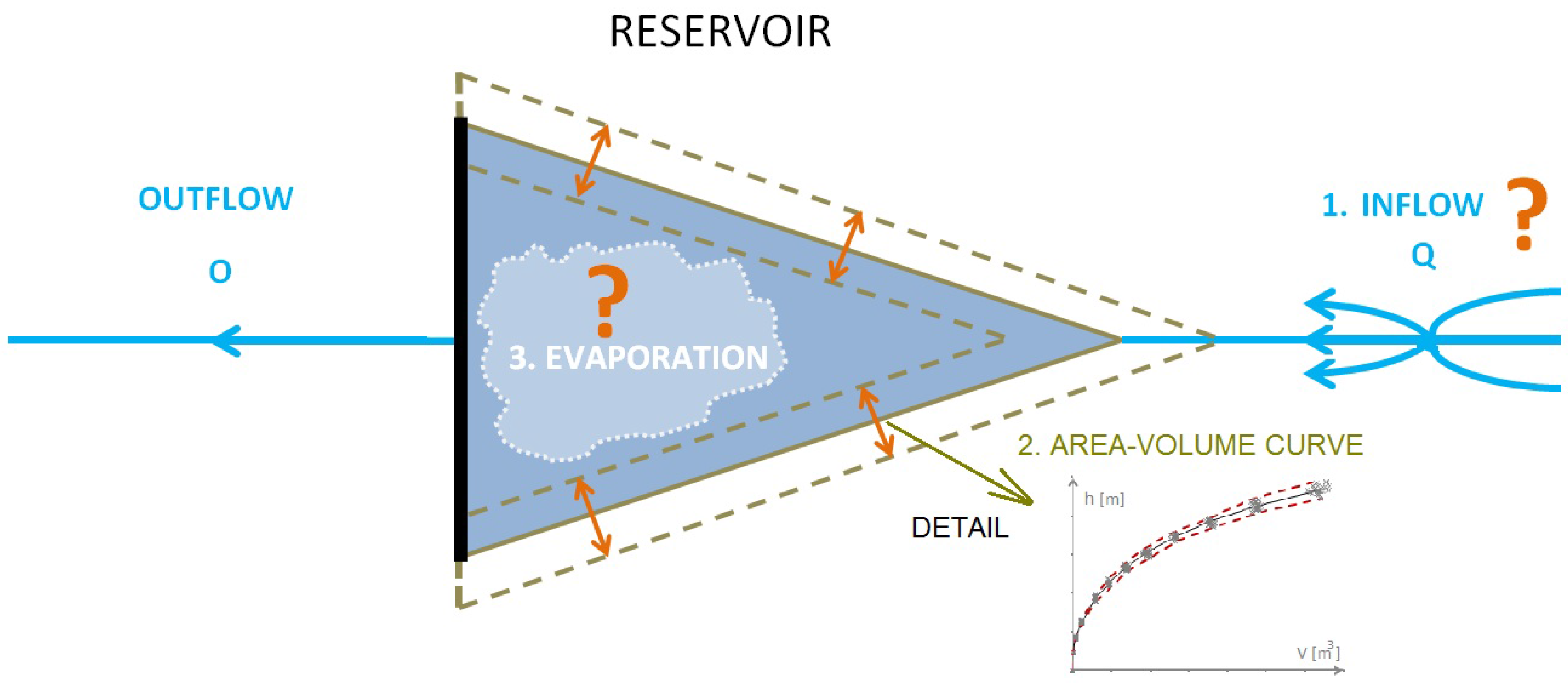
The novelty of this paper is on right selection of uncertainty, suitable for reservoir design and the application of all knowledge in follow-up publications [13] and [21]. Based on this information, the method, algorithm and user interface are developed. This methodology allows the generation of uncertainty together or separately as an individual source of uncertainty. Using correct data, the described method will allow the design of a new reservoir capacity under conditions of hydrological uncertainty including water losses. The aim of the paper is to use the existing knowledge to introduce uncertainties of input hydrological, morphological, and operational data required for the design of the reservoir storage capacity and for the calculation of hydrological reliability of the water outflow from the reservoir. The methodology will be applied on the reservoir design in the protected profile of Hanušovice on the Morava/Krupá River.

2. Methods

2.1. Monte Carlo Method

The general methodology for generating uncertainty affected hydrological, morphological and operating input data for the related water management analysis of a reservoir for its storage capacity was described in [21]. Generally, uncertainties of input quantities are introduced into the calculations using the Monte Carlo method. Using cumulative distribution function F(X) and a random number generator, random positions of values NX_i corresponding to the interval of initial uncertainty are generated. Value X_i is considered as a random and independent value to the values X_i-1 and X_i+1. This presumption allows the use of the normal probability distribution N(μ(X),σ(X)). Then, the input value X_i is considered as the mean μ(X) and uncertainty size is defined as the standard deviation σ(X). Subsequently to each mean μ(X_i), a cumulative distribution function F(X) of the standard normal probability distribution is created. The random number generator creates random numbers from the interval and then the position of the random value NX_i is calculated.

The basic principle of generating random positions of (NV_i, Nh_i) is similar to the above mentioned theory. The difference is given by the construction of random points which requires building two independent Monte Carlo generators. Each generator will design a random position of point NX_i (e.g., water level elevation Nh_i) and will add a random value NY_i to it (of the water volume in the reservoir NV_i). For the line of the area–volume curve, the result is a random point coordinate (NV_i, Nh_i) of the line of the elevation–volume curve, see Figure 1.

From the point of view of the Monte Carlo simulations, the main differences from the publications [13] and [21] are in the data which enters into the reservoir simulation model. Regarding the design of a reservoir, water seepage it is not considered in calculations such as those in [21]. In addition, neither is extended hydrological data in form of artificial time series based on AR and ARMA models considered [13]. The uncertainty is applied on the inflows into the reservoir; the water evaporation losses from the reservoir, the reservoir elevation–volume curve and the reservoir elevation–area curve are considered as hydrological and operating inputs. The principle of introducing uncertainty into the calculation of the active reservoir conservation storage capacity is shown in Figure 2.

The application of uncertainties into the input data gives rise to generated random water inflows into the reservoir, random water evaporation from the reservoir and a random reservoir elevation–volume curve and reservoir elevation–area curve. These random ensembles serve as input values for a simulation model which uses single-pass simulation of the reservoir behavior in the conditions of data uncertainties.

2.2. Reservoir Simulation Model and Reliability Assessment

The reservoir simulation model was developed based on Starý (1995) [22], and in [17], the methodology was extended by the Monte Carlo simulation approach. The basis for the reservoir simulation model is an adapted reservoir equation in the summing form converted into the following Equation (1) [22]. Equation (1) is used in the simulation reservoir model for the calculation of the reservoir storage volume at 100% reliability of water outflow from the reservoir. Equation (2) [22] provides a basis for calculations of hydrological reliability.

$$0\le {\displaystyle \sum }_{i=0}^k\left(O_i-Q_i\right)\Delta t+\left(O_{i+1}-Q_{i+1}\right)\Delta t$$

(1)

$$0\le {\displaystyle \sum }_{i=0}^k\left(O_i-Q_i\right)\Delta t+\left(O_{i+1}-Q_{i+1}\right)\Delta t\le V_{z,max}$$

(2)

where O_i is the water outflow from the reservoir, Q_i is the water inflow into the reservoir for i = 1, …, k, Δt is the time step of the calculation (one month). O_i+1 is the water outflow from the reservoir in the subsequent time step in step i+1. If the sum in (1) and (2) is less than zero, the value O_i+1 will be substituted by the value of the reservoir outflow or water demand, called the required improved outflow O_p. The required outflow O_p is defined as the total outflow from the reservoir. In times of inflow water deficit, when the storage capacity is using for water supply, the required outflow consists of ecological outflow Q_ECO and water consumption for water supply. The time course of the calculated sum simulates the course of the emptying of the reservoir storage volume by time steps i = 1, …, k. For i = 0, the initial condition of the solution needs to be entered after the sum value.

Equation (2) is limited from the left by value 0, which represents the full storage capacity and from the right side, it is limited by the V_Z,max empty storage capacity. These boundaries characterized the active conversation storage capacity, which is possible to use. From the argument calculation in (2), the actual emptying of the reservoir is obtained, called V’_Z,i+1, which is then tested if it is in a given interval 〈0,V_Z,max〉. If not, it is important to find the value O_i+1, when the argument in the summation is equal to zero—then, a manipulated outflow is created, or a given argument is equal V_Z,max—a failure or unsatisfactory state is created.

A general definition of the reliability of the water management system has been successively described by Kritskiy and Menkel (1952) [23], Klemeš (1967) [24] and Hashimoto (1982) [25]. Classification of the failure of the reservoir storage volume for the subsequent calculation of reliability is as follows Equation (3)

$$Z_{t,i}=\{\begin{array}{c}{Z}_{t,i}=1,O_i\ge O_P\\ Z_{t,i}=0,O_i<O_P\end{array}$$

(3)

where Z_t,i = 1 describes the state of the reservoir storage capacity in the satisfactory time step of the calculation. Z_t,i = 0 describes the state of the reservoir storage capacity in the unsatisfactory (failure) time step of the calculation. The given reliability used in the paper is known as temporal reliability or time based reliability and can be calculated from Z_t,i values. Each value Z_t,i represents a month. The reliability R_T is defined as Equation (4)

$$R_T=\frac{1}{k}{\displaystyle \sum }_{i=1}^k{Z}_{t,i}$$

(4)

where k is the number of all months for the given solution of time series.

Generated random ensembles of water inflows into the reservoir, water evaporations from the water level, and random curves of area–volume curves are repeatedly read by the simulation reservoir model. The simulation model makes calculations of the reservoir storage volume both with and without considering water losses from the reservoir. The repeated calculations result in a range of reservoir storage volumes for 100% reliability. Furthermore, the hydrological reliability in the form of R_T time-based reliability is calculated. These sets of simulation results are further statistically evaluated. Basic statistical analysis consists of a statistical histogram and statistical characteristic; (i) the mean value μ, (ii) dispersion D, (iii) standard deviation σ, (iv) variation coefficient C_v and (v) excess coefficient C_a.

Different to publications [13] and [21] is the storage capacity analysis. In [13], the storage capacity analysis with 100% reliability with no water losses was made. The methodology was applied on a fictive water reservoir. In [21], the reliability analysis on the existing reservoir Vir I was described. For this kind of analysis, the historical measurements and data in the form of time series of water inflow, evaporation historical data, and actual area–volume curves data were available. Further, the practical application of the uncertainty analysis of storage capacity to a new design of reservoir will be performed. Water management planning, as described in [26], is conducted in the site area.

3. Practical Application

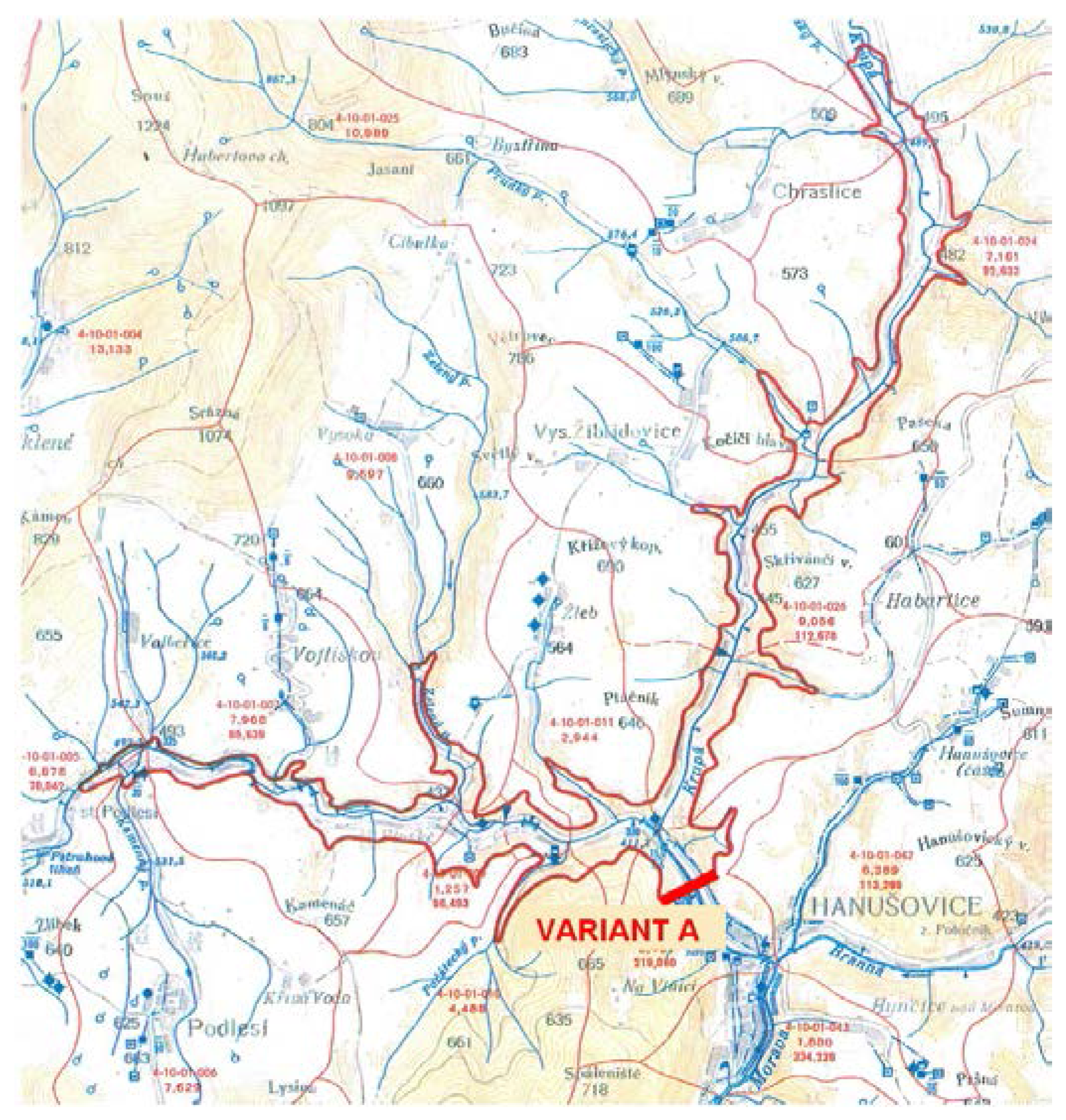
Practical application is based on the needs for a feasibility study of variants for the open water reservoir Hanušovice. The Morava River Basin Authority has commissioned a study of a water management solution for the Hanušovice reservoir in order to enhance the water supply purposes of the regions in the north-east part of the Czech Republic. The presented results of calculations are done for the intended variant A—a large reservoir below the confluence of Morava and Krupá Rivers, see in Figure 3.

The input values for the calculation were constituted by the time series of the mean monthly flow in the duration of 66 years for the time period of 1950 to 2014 in the profiles of Vlaské on the Morava River and Habartice on the Krupá River. Both profiles are operated and data is managed by CHMI (Czech Hydrometeorological Institute). 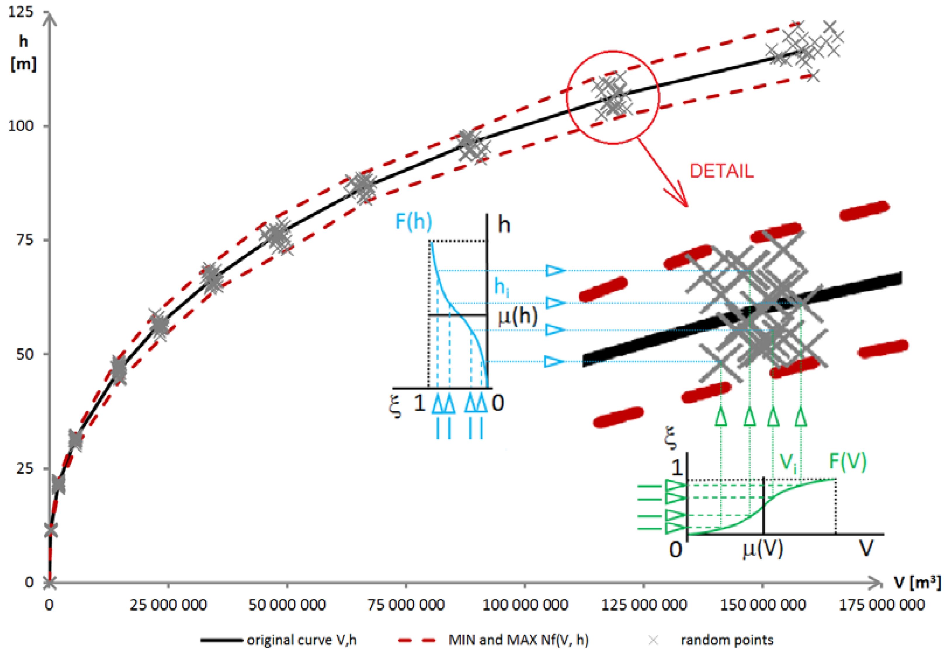The mean annual evaporation E_a was consequently divided among individual monthly values of evaporation according to the standard Reservoir storage capacity analysis (ČSN 75 2405, 2004) [27]. Bathymetric curves are determined using the GIS software and a DTM—Digital Terrain Model.

The reservoir is designed with regard to the calculation of the storage volume V_z for 100% reliability. Furthermore, the reliability of the reservoir storage volume is analyzed, as well.

The value of annual evaporation from the water level E_a is 700 mm from the estimated water level altitude of approximately 460 m a.s.l. Improved outflow from the reservoir O_p ranged between 0.6 and 0.8 (60% to 80%) of the reservoir yield. According McMahon and Adeloye [28], the yield is the controlled release from the reservoir system and is often expressed as a ration or percentage of the mean annual inflow to the reservoir. During calculation, many different possibilities of reservoir yield have tested. A yield interval from 0.6 to 0.8 is taken into account according to the best utilization of water inflow conditions. The input value of extended uncertainty of the storage volume is entered constantly for all parameters within the range of ±6% and ±9%. For all uncertainties, a uniform distribution is considered. The presented initial uncertainty evaluation is considered as more conservative, rising from uncertainty of measurement. The number of repetitions of random input parameter generation using the Monte Carlo method equaled 300. A total of 300 repetitions were done due to two reasons: first, better statistical evaluation; second, 300 repetitions is the best ratio between the value according to computation time and the accuracy of results. For these two reasons, the different number of repetitions was tested.

The designed reservoir profile is located below the confluence of the Morava and Krupá Rivers; the closest water measuring profile is Raškov. The flow series for the reservoir profile was considered in a simplified way as the sum of the flow series Vlaské and Habartice. The effect of the sub-basin between the profiles was neglected. The mean long-term annual flow Q_a is 4.087 m³·s⁻¹.

4. Results

Table 1. Reservoir storage volume considering uncertainties for 100% reservoir reliability.

Uncertainty		±6%			±9%
yield	OP (m3·s-1)	μ(Vz) (m3)	3 σ(Vz) (m3)	3 σ(Vz) (%)	μ(Vz) (m3)	3 σ(Vz) (m3)	3 σ(Vz) (%)
0.6	2.453	27 764 638	±638 831	±2.30	27 823 438	±903 776	±3.25
0.7	2.861	44 111 900	±1 830 159	±4.15	44 105 676	±2 742 899	±6.22
0.8	3.270	68 148 752	±1 831 426	±2.69	68 148 040	±2 756 372	±4.05

shows the results of calculations of the reservoir storage volume for a reservoir yield from 0.6 to 0.8 and 100% reliability of the reservoir storage volume. The value μ(V_z) is considered as the result of the calculation following statistical evaluation. The value 3σ(V_z) subsequently shows the value of maximum uncertainty of the storage volume covering 99.97% of the volume occurrence probability in the observed set of realizations.

For the calculation of temporal reliability of the reservoir volume, the reservoir storage capacity is entered from the calculation of a deterministic solution and corresponds to the value of 44,127,380 m³ for the reservoir yield 0.7. Dead space is considered as 10% of the storage volume. Due to the uncertainties entered into the calculation, for the reservoir yield yield = 0.7 the resulting reliability is not R_T = 100% as mentioned in Table 1 but only 99.90% for both input uncertainties ±6 % and ±9 %. In order to achieve 100% reliability for uncertainty ±6 %, we must decrease the required outflow, in particular, to yield = 0.693, and for uncertainty ±9 % even down to yield = 0.690. The decrease is determined by the randomness of input values, or input uncertainty which in a certain number of cases undervalues the series, thereby also causing the decrease of the value of reliability.

Table 2. Calculation of temporal reliability of water outflow from the reservoir considering the input uncertainties.

Uncertainty		±6%			±9%
Yield	OP (m3·s−1)	μ(RT) (%)	2 σ(RT) (%)	3 σ(RT) (%)	μ(RT) (%)	2 σ(RT) (%)	3 σ(RT) (%)
0.690	2.819	100.00	±0.00	±0.00	100.00	±0.00	±0.00
0.693	2.833	100.00	±0.00	±0.00	99.99	±0.05	±0.07
0.70	2.861	99.90	±0.21	±0.32	99.90	±0.23	±0.34
0.72	2.943	99.62	±0.03	±0.04	99.63	±0.07	±0.11
0.73	2.984	99.53	±0.12	±0.18	99.54	±0.13	±0.20
0.74	3.025	99.30	±0.18	±0.26	99.29	±0.24	±0.36
0.76	3.107	98.49	±0.14	±0.22	98.52	±0.21	±0.31
0.78	3.188	98.06	±0.22	±0.33	98.02	±0.25	±0.38

represents the results of the analysis of reservoir reliability calculations. The value μ(R_T) is considered as the result of the calculation; the values 2σ(R_T) and 3σ(R_T) then describe the size of uncertainty occurring around the result of the calculation. The analysis has been done for the reservoir yield values of 0.7 to 0.78.

In the first round of calculations, reservoir storage volumes have been determined for the sizes of improved outflow corresponding to the reservoir yield of 0.6 to 0.8. Temporal reliability of water outflow from the reservoir is calculated. The volume that defined the boundary of the maximum storage volume determining the limit bounds of reservoir failure, or rather, reservoir emptying, corresponded to the volume for the reservoir yield 0.7.

In the designed profile, the outflow corresponded to O_p = 2.861 m³ s^-1 for the reservoir yield = 0.7. For the mentioned outflow, the storage volume is calculated for 100% reliability of water outflow from the reservoir. The results can be interpreted as follows. The mean value of the storage volume is considered as the resulting value. During the check of the calculation correctness, the storage volume has calculated also for the deterministic solution. Its value is almost identical to the calculation in the stochastic solution. In the deterministic solution, the storage volume is V_z = 44,127,380 m³. If, along with the results, we also consider the uncertainties entering the solution, the results will become markedly skewed. The storage volume with consideration of input uncertainties corresponding to the value 3σ∙μ(V_z) can be presented this way. For the value of input uncertainty ±6%, the storage volume lies within the interval V_Z∈〈42,281,741 m³; 45,942,059 m³〉 with the volume uncertainty being ±4.15%. For ±9% of input uncertainty, the volume range exceeds ±6% of the uncertainty interval. The storage volume ranges within V_Z∈〈41,362,777 m³; 46,848,575 m³〉.

The temporal reliability considering input uncertainties may be considered for the input uncertainty of ±6% and O_P = 2.984 m³ s^-1 as R_T = 99.53% ± 0.18%, or in other words, it will lie within the interval R_T∈〈99.35%; 99.71%〉; and R_T = 99.54% ± 0.20% then works out for ±9% of the input uncertainty, or in other words, it lies within the interval R_T∈〈99.34%; 99.74%〉.

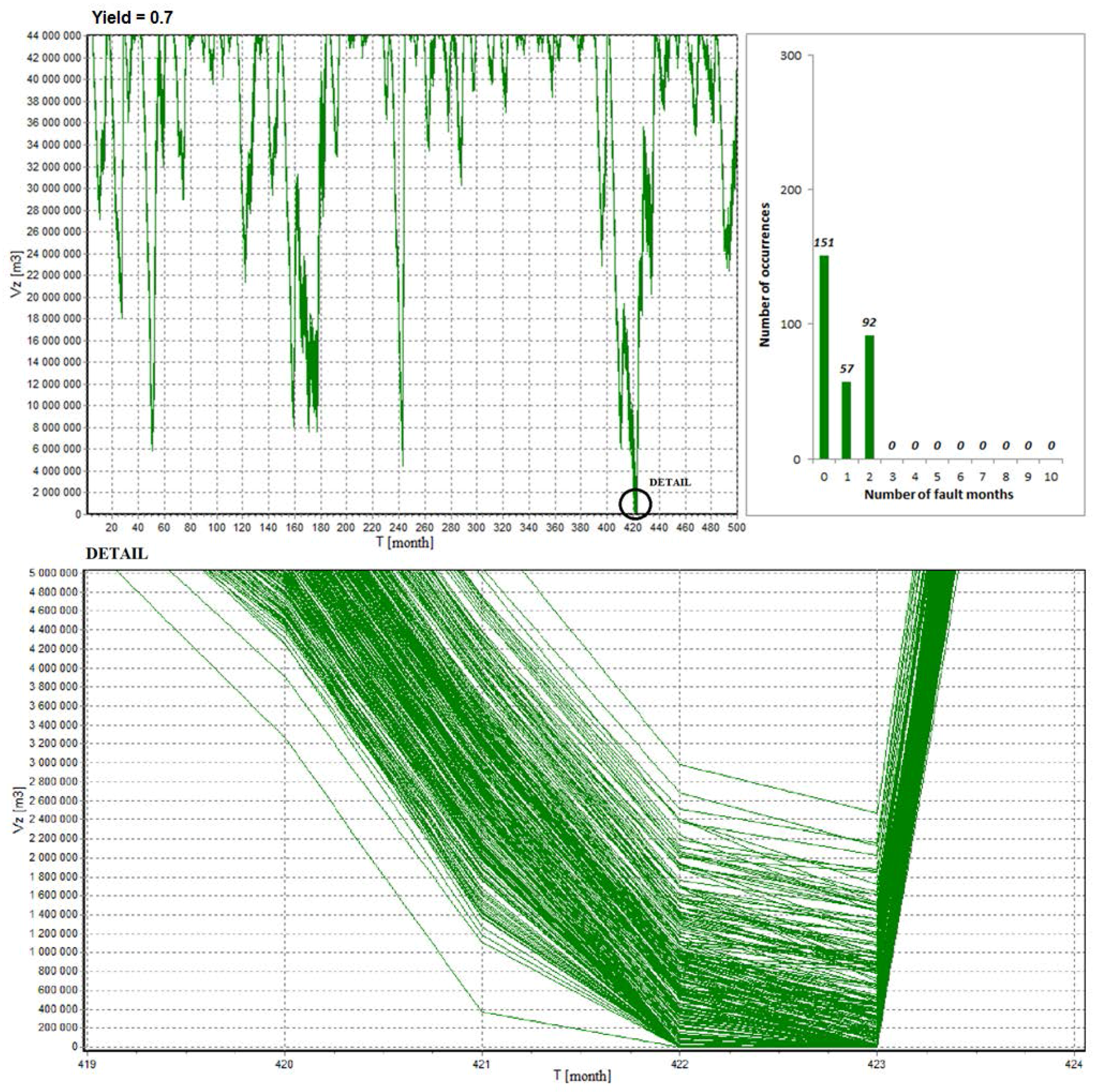
Figure 4 describes the course of reservoir filling considering water losses from the reservoir for the initial uncertainties of ±9% and for the reservoir yield yield = 0.70. The histogram next to the course shows the distribution of numbers of failure months in the course of the calculation.

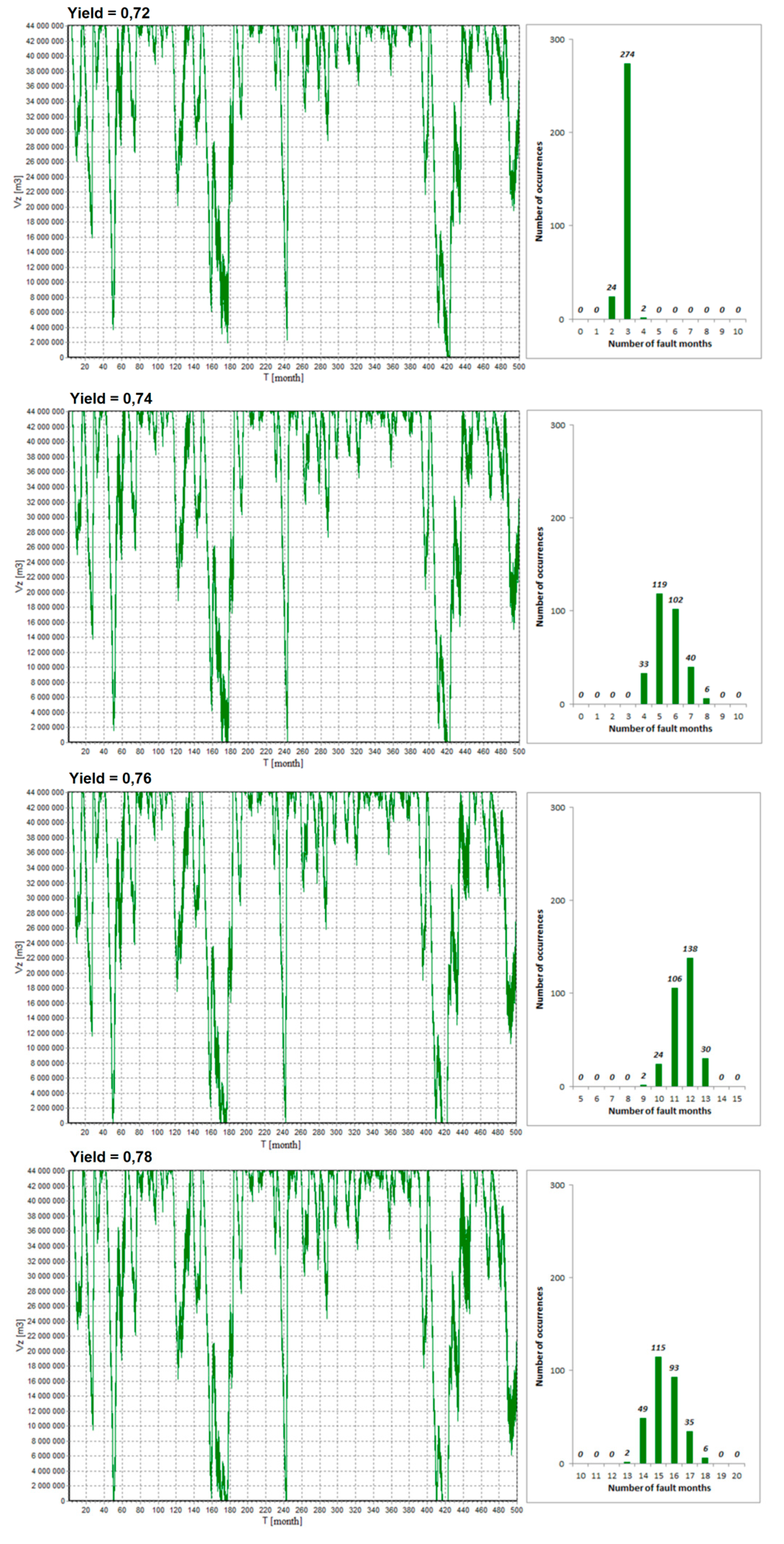
Also Figure 5 shows analysis of the course of reservoir filling considering water losses from the reservoir for the initial uncertainties of ±9% and histograms for the reservoir yields yield = 0.72, 0.74, 0.76 a 0.78.

5. Conclusions

As first, it is important to say that Czech national standards [27] valuated open water reservoirs into the classification based on their strategic importance. Each class—Class A, B, C, D—is defined by strategic importance in the water distribution system and is evaluated by time-based reliability. Class A–R_T ≥ 99.5%, B–R_T ≥ 98.5%, C–R_T ≥ 97.5%, D–R_T ≥ 95%.

Based on further processed results presenting courses of reservoir filling and emptying with histograms of failure months, we can present the temporal reliability also on the basis of the occurrence frequency of failure months.

For example, from the histogram in Figure 4, where the yield 0.7 is, it seems that reliability R_T = 100.00% corresponds to the random ensembles with there being a 50.33% probability of zero failure month occurring, that is 151 random ensembles from 300 repetitions. Reliability R_T = 99.87% corresponds to the random ensembles with there being a 19.00% probability of one failure month occurring, that is 57 of 300. Reliability R_T = 99.74% corresponds to the random ensembles with there being a 30.67% probability of two failure months occurring, that is 92 of 300 repetitions. In general, it can be said that the reliability complying with the highest category of reservoir operational reliability according to Czech legislation Category A - R_T ≥ 99.5%, will be attained or exceeded with a 100.00% occurrence of probability, or in other words, all 300 random ensembles agree with this requirement. Interpretation of results as per Table 2 can be described in the following way. Reliability with the assumption 3σ (99.97% occurrence probability) for the same case, i.e., uncertainty ±9% and O_P = 2.861 m³·s⁻¹ is R_T = 99.90 ± 0.34% or R_T∈〈99.56%; 100.00%〉. This interval will also comply with the whole range of Category A.

For example, the histogram in Figure 5, for yield 0.72, we can say that reliability R_T = 99.74% corresponding to the random solution with two failure months will occur with an 8.00% probability, that means 24 ensembles from 300 repetitions. Reliability R_T = 99.62% corresponding to the occurrence of three failure months in the random solution will correspond to a 91.33% occurrence probability, or 274 of 300. For four failure months, the reliability is R_T = 99.48%, corresponding to a 0.67% occurrence, which falls upon only two random solutions out of 300. Category A defined will be attained or exceeded with a 99.33% occurrence probability, or in other words, 298 random ensembles out of 300 will meet this requirement. On the contrary, a solution not complying with Category A but still complying with Category B (R_T ≥ 98.5%) will occur with a 0.67% probability—that means, only in two cases out of 300. As per Table 2 and again input uncertainty ±9% and O_P = 2.943 m³·s^–1 is R_T = 99.63 ± 0.11% or R_T∈〈99.52%; 99.74%〉. This interval will comply with the whole range of Category A of hydraulic structure reliability.

From the perspective of class A, the other results are not relevant, because for other yields—0.74, 0.76 and 0.78—the four months failure occurred in all ensembles and they are out of class A. It is clear that Table 2 shows the same results. Reliability corresponding yields 0.74, 0.76 and 0.78 are out of class A. From the perspective of class B, 11 failure months or more are interesting for another reason. In the case of yield = 0.74, it can be classified to class B results, in the interval R_T∈〈98.93%; 99.65%〉; however, in yield = 0.76, there are 56% random ensembles, 168 cases of ensembles from 300, out of class B. Yield = 0.78 is out of class B for all random ensembles.

Based on the obtained results, it seems, in Table 1 and Table 2, that it is possible that the values of both the storage capacities and the reliability, determined without considering input data uncertainty, may be markedly undervalued. Under certain conditions, a reservoir may even be misclassified into a significance (reliability) class of hydraulic structures [27] for purposes of water supply, and thereby its operational capacity may be compromised in water deficient and dry periods. The consequence may be apparent in the form of an operational failure of the storage volume. As can be seen in Table 2, for given cases, yield = 0.72 mean values of reliability equal 99.53% and 99.54% but the occurrence interval unequivocally falls under the weighed limit of 99.5%. A problem arises here with unequivocal classification of the reservoir into a category of reliability.

Another problem is the correct calculation and design of the flood protection volume of the reservoir, the location of the height of the top of the dam and the associated future costs of reservoir construction. For this reason, a preliminary design of the reliability overflow has been worked out, and the volume size of the reservoir flood protection capacity has been determined. The known design flood hydrogram was used. Based on the hydrogram volume, a given reservoir volume for yield = 0.7, and the area–volume curve, the reservoir flood protection volume of 5.5 hm³ has been designed. If we consider the resulting storage volume corresponding to the value of 44.1 hm³ and an uncertainty of ±2.7 hm³, then the reservoir flood protection volume may be up to a half affected by the uncertainty of the storage capacity design. This also relates to the design of the height of the top of the dam which can be approximately ±1.2 m of the total dam height. Figure 6 shows the connection of the uncertainty of the reservoir storage volume to all the design and operation parameters of the reservoir.

If we want the solution to be secure on the side, it is necessary to add the resulting uncertainty of the reservoir storage volume to the volume. However, that consequently places demands on the size of the reservoir body and on the total costs of the possible construction. It must also be added that uncertainty of the input parameters were not considered in the solution of the reservoir retention volume. For example, uncertainties of flood flows were neglected which may reach up to 10% to 20% values.

At present, the results cannot be generalized. However, the algorithm is written universally and may be used for other reservoirs as well. While performing the sensitivity analysis, the same initial uncertainty values are always counted for all input data. That means that the initial uncertainty ±6% and ±9% is used. For future work, it is necessary to conduct an uncertainty analysis for each source of uncertainty separately; to evaluate which input data and its uncertainty influenced storage capacity more; whether the water inflow is the most significant source of uncertainty or not; and how other input uncertainties affect the result. For example, in the present study, it is unknown which uncertainty values may be reached by, e.g., courses of the area–volume curves, when their stated current course is affected by reservoir clogging and other influences. Here, it may be assumed that higher uncertainty in the course of the bathymetric curve may influence the results more. From the mentioned point of view, the results may differ, and therefore the intervals describing the occurrence of calculated reliability R_T may differ, as well.