Article

Estimating the Probability of Vegetation to Be Groundwater Dependent Based on the Evaluation of Tree Models

by
Isabel C. Pérez Hoyos
*,
Nir Y. Krakauer
and
Reza Khanbilvardi
National Oceanic and Atmospheric Administration-Cooperative Remote Sensing Science and Technology (NOAA-CREST) Center, The City College of New York, New York, NY 10031, USA
*
Author to whom correspondence should be addressed.
Environments 2016, 3(2), 9; https://doi.org/10.3390/environments3020009
Submission received: 28 January 2016 / Revised: 10 March 2016 / Accepted: 22 March 2016 / Published: 2 April 2016
(This article belongs to the Special Issue Data-Modelling Applications in Water System Management)

Abstract

:
Groundwater Dependent Ecosystems (GDEs) are increasingly threatened by humans’ rising demand for water resources. Consequently, it is imperative to identify the location of GDEs to protect them. This paper develops a methodology to identify the probability of an ecosystem to be groundwater dependent. Probabilities are obtained by modeling the relationship between the known locations of GDEs and factors influencing groundwater dependence, namely water table depth and climatic aridity index. Probabilities are derived for the state of Nevada, USA, using modeled water table depth and aridity index values obtained from the Global Aridity database. The model selected results from the performance comparison of classification trees (CT) and random forests (RF). Based on a threshold-independent accuracy measure, RF has a better ability to generate probability estimates. Considering a threshold that minimizes the misclassification rate for each model, RF also proves to be more accurate. Regarding training accuracy, performance measures such as accuracy, sensitivity, and specificity are higher for RF. For the test set, higher values of accuracy and kappa for CT highlight the fact that these measures are greatly affected by low prevalence. As shown for RF, the choice of the cutoff probability value has important consequences on model accuracy and the overall proportion of locations where GDEs are found.

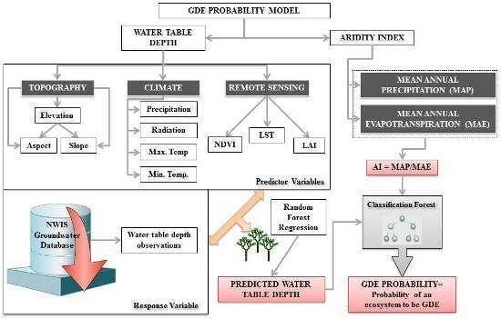
Graphical Abstract

1. Introduction

Groundwater Dependent Ecosystems (GDEs) are defined as communities of plants, animals, and microorganisms that use the groundwater resource for the maintenance of their structure and function [1,2]. GDEs include some types of wetlands, springs, rivers, and terrestrial vegetation (together with the fauna they support). A simple classification of GDEs was suggested by [2]:
  • Ecosystems dependent on the surface expression of groundwater: this category includes springs, “minerogenous” wetlands (wetlands supported by groundwater that has been in contact with mineral soils or bedrock), river baseflow systems, and some estuarine and near-shore marine ecosystems that depend on the near-shore discharge of groundwater.
  • Ecosystems dependent on the subsurface expression of groundwater: terrestrial vegetation that uses shallow groundwater (commonly referred to as phreatophytes). The water table can be considered shallow if it is less or equal to 10 m in depth [3], intermediate if it is between 10 m and 30 m, and deep if it is greater than 30 m. Plants can access groundwater by extending their roots to the water table and capillary fringe right above it. The roots of phreatophytes extend up to 3 m to almost 15 m below the land surface depending on the species [4].
  • Aquifer and cave ecosystems: these include fractured rock, karstic, and alluvial aquifers, hyporheic zones of rivers and floodplains (saturated interstitial area beneath and alongside a stream bed where shallow groundwater and surface water mix), and stygofauna (organisms living in groundwater systems or aquifers).
GDEs are of vital importance for the conservation of biodiversity, maintenance of water quality, prevention of soil erosion, and carbon sequestration [1,2]. Unfortunately, their degradation has been increasing over the past decades due to humans’ rising demand for water to sustain agricultural activities and support industrial expansion, economic development, and population growth [5]. As a result of surface water supplies not being enough to meet these demands, there is a growing risk of depletion and contamination of groundwater resources that could eventually lead to alterations in vulnerable GDEs. Consequently, there is an imperative need to identify the location of GDEs.
The first step in the protection of GDEs is their delineation, followed by identification of systems at risk and groundwater stress indicators. Currently, the biggest challenge in the conservation of GDEs is that information about the location of these ecosystems is required and although it might be available at local scales, there is little information for larger scales [6]. Australia and South Africa are the only two countries that have developed national inventories of GDEs. In Australia, an operational GDE atlas was produced by combining previously identified GDEs, available literature, geospatial layers, and remote sensing data [7]. In South Africa, a national scale map of GDEs depicting the probability of occurrence of terrestrial GDEs according to groundwater levels and the duration of the moisture growing season was created [8]. Unfortunately, the assessment with the largest extent that has been undertaken for the United States only depicts phreatophytic land cover of the northern and central Great Basin Ecoregion [4].
Identification of GDEs as part of ecological inventories and mapping of ecosystems is typically accomplished with the collection of field survey data. Over the past four decades, remote sensing technologies have advanced drastically and have become critical for a variety of ecological applications, including ecosystem mapping. Several studies have utilized geographic information systems (GIS) to analyze satellite imagery because of their ability to implement spatial models that combine key factors affecting ecosystem distribution [8,9,10,11,12].
Many of these efforts have defined indices of groundwater dependency by ranking ecosystems according to geomorphological, ecological, and hydrogeological criteria [8,13,14]. Modeling approaches that are commonly used in ecology for predicting the probability of occurrence of species [15,16] have been explored for different applications, such as the assessment of hydrological and land use aspects that influence the occurrence of riparian and floodplain tree species [17]; prediction of the response patterns of grassland species to changes in soil moisture and water level [18]; evaluation of the response of groundwater-connected riverine grassy woodlands to drought conditions [19]; and the prediction of forest dieback [20]. Predicted species distributions are based on models of relationships between species occurrence survey data (response variables) and environmental factors (predictor variables) [21]. In the context of GDEs, the combination of satellite imagery and field survey data can be used to create a proxy for the location of groundwater dependent ecosystems. A comprehensive review of the methods used to map GDEs with a focus on studies that have benefited from geospatial technologies for mapping GDEs at different extents is provided in [22].

1.1. Ecohydrology of GDEs

Since at least the beginning of the 20th century, vegetation gained attention as strong indicator of groundwater presence. Reference [23] utilized information about plants along with groundwater data to investigate the ecohydrology of GDEs. Ecohydrology is defined as the description of the hydrological mechanisms that underlie ecological pattern and processes [24]. The hydrology of GDEs is characterized using four different aspects of the groundwater regime [25], namely level, flux, pressure, and quality [26]. GDEs have a strong connection with rainfall, groundwater, and soil water content, which leads to important feedbacks between ecosystems and hydrological processes. The dynamics of GDEs are controlled by the coupling of soil moisture dynamics and water table depth, and are strongly influenced by capillary rise, and plant water uptake [27]. Studies concerning the links between vegetation, precipitation, and soil water content for water-limited ecosystems (where groundwater is too deep to influence the soil water balance) [28,29,30,31,32,33,34] have been essential in understanding the association between soil water content and many hydrological and bioecological processes (e.g., precipitation, infiltration, plant transpiration, and nutrient cycling) [35]. However, for the characterization of the ecohydrology of GDEs, frameworks that are able to provide quantitative tools to investigate the interactions between shallow aquifers and soil moisture dynamics are required [36]. GDEs are considered humid ecosystems because groundwater influences the soil water balance. Humid ecosystems are characterized as being strongly controlled by interactions between vegetation water use and groundwater [37]. When plants have constant or intermittent access to groundwater, they respond to changes in water table depth [2]. Easy access to groundwater can considerably increase its use by vegetation and the development of dependence on the groundwater resource. In the case of GDEs, water use can potentially be higher than the local rainfall input, and groundwater may comprise a large percent (more than 50%) of annual transpiration [37]. According to [2], groundwater dependency by terrestrial vegetation can be quantified using a water budget approach. If the total amount of water that is being used by plants in a given site for a year can be demonstrated to be considerably larger than the annual available rainfall for the site, it can be concluded that groundwater is being used by the ecosystem. On the other hand [38,39,40], the presence of ecosystems dependent on the subsurface expression of groundwater is linked to locations where groundwater is accessible to vegetation, i.e., is relatively shallow.

1.2. Research Objectives

This study consists in the evaluation and comparison of classification trees (CT) and a random forest (RF) algorithm for estimating the probability of an ecosystem to be groundwater dependent (GDE probability) at 1 km spatial resolution. The focus of this paper is to identify ecosystems that are dependent on the subsurface expression of groundwater (hereafter referred to as “GDEs”). The term GDEs will be used in this manuscript to refer to phreatophytes, and it will not include wetlands, rivers, springs, and other types of ecosystems that might be dependent on groundwater. The CT and RF modeling techniques are applied for the state of Nevada, USA, to develop a systematic approach for identification of GDEs. The product can potentially be used for the definition of conservation areas since the resulting predicted probability map can be translated into a binary classification map with two classes: GDE and NON-GDE. Such a map can be created by selecting a probability threshold (also called cut-off value). We demonstrate that the choice of this threshold has dramatic effects on deterministic model performance measures [41]. Finally, a brief assessment of considerations for threshold selection based on different groundwater management scenarios is also provided.

2. Materials and Methods

2.1. Study Area

The study area is the western state of Nevada, USA, and comprising 110,567 square miles. Nevada primarily includes desert and semiarid climate regions and it is characterized by abrupt changes in elevation, with the presence of both high mountains and flat arid valleys [42]. Nevada was selected as the study area because of its geomorphological contrasts, wide range of climatic conditions that have led to the presence of a great variety of vegetation types, and known presence of GDEs [43].
Prediction of GDE probability is accomplished by modeling the relationship between the known locations of GDEs and two key factors that likely influence the distribution of GDEs, namely water table depth (WTD) and aridity index (AI). Other factors such as land cover, land use practices, surface water dynamics, and water quality are important for the characterization of the response of GDEs [44], evaluation of the impacts of natural events and anthropogenic actions on GDEs [17,20,45], and for estimating the volume of groundwater required by GDEs [46]. However, these factors are not included in our simplified model framework. Probability estimates are generated for a 1 km grid cell resolution, based on the resolution of the geospatial data layer inputs. The modeling approach selected for the development of the GDE probability map results from a comparison of the performance of two models that have been widely used for predictive mapping CT and RF. Predictive performance evaluation for the selection of the most accurate model is done using a threshold independent technique, and the prediction accuracy of both models is assessed in greater detail using threshold-dependent measures.
The implementation of the tree models (CT and RF) within a GIS interface is achieved with the use of Marine Geospatial Ecology Tools (MGET). This toolbox was developed by the Marine Geospatial Ecology Laboratory at Duke University [47]. MGET is a free, open-source geoprocessing toolbox suitable for ecological research, conservation, and spatial planning problems. MGET applies the classification tree and random forest algorithms by integrating with ArcGIS [1] the rpart package [48] and RF package [49] available in the R environment for statistical computing [50] with ArcGIS [51].

2.2. Predictor Variables

WTD information will be integrated with the AI developed by the United Nations Environment Program [52]. WTD prediction is accomplished with the RF regression algorithm using climatic, topographic, and vegetation information as predictor variables, and depth to groundwater records as response variables. Water table depth observations are available at 567,946 sites in the United States from 1927 to 2009. These observations are taken from a data set that includes only shallow wells, less than 100 m in depth, in unconfined aquifers hydraulically linked to the land surface [53]. For this study, only observations in Nevada were used (6483 sites). The depth to groundwater records used for the analysis are the average WTD values for each site, with different sites having different numbers and periods of observations. Calculated WTD is shown in Figure 1. Additional information about the derivation of the spatially continuous WTD values can be found in two companion papers [42,54].
The AI is a numerical climate-based indicator for a deficit of available water. A variety of aridity indices have been proposed, but a widely used recent index was developed by the United Nations Environment Program [52]. This estimator is defined as the ratio between Mean Annual Precipitation (MAP) and Mean Annual Potential Evapotranspiration (MAE). In other words, the AI quantifies precipitation availability relative to atmospheric water demand with the purpose of providing a depiction of the rainfall deficit for potential vegetative growth. The Consortium for Spatial Information (CGIAR-CSI) Global-Aridity database was developed based on the UNEP definition of AI with the support of the International Water Management Institute (IWMI) and the International Centre for Integrated Mountain Development (ICIMOD) [55,56]. This database is made available through CGIAR-CSI website (http://www.cgiar-csi.org) at 30 arc second (~1 km at the equator) resolution. The AI calculated using this method is divided into categories based on the classification originally developed by the UNEP. Based on the UNEP categories, Nevada ranges from arid to humid climate (Figure 2). The use of AI for identifying GDEs relates to the perspective of water balance. If the AI value is low (<0.5), that means that the MAE is much higher than the MAP, so that plants will not be able to freely transpire and grow over at least a large part of the year unless additional water sources such as groundwater are available to them.
To check for possible multicollinearity, the correlation between AI and WTD was calculated. A low correlation coefficient (0.032) was obtained. This has important implications for the results obtained from CT, because this algorithm is negatively affected by predictor variables that are correlated (in this case correlation is very weak). If AI and WTD were strongly correlated, the resulting tree would be unstable to small perturbations in the dataset, increasing the likelihood that different solutions will be obtained across samples [57].

2.3. Response Variable

The response (also known as dependent variable) here is a binary variable, represented as 0 for pixels that are identified as non-GDE (groundwater dependence absence) and 1 for pixels identified as GDEs (groundwater dependence presence). Using toolboxes available in ArcGIS 10.2, the three datasets that can be used as indicators for the occurrence of GDEs (Table 1) are reclassified into two categories (0 or non-GDE, and 1 or GDE) to obtain the response variable surface map. These datasets are described in detail in the immediately following paragraphs. The three datasets map the presence of phreatophytic species that are commonly found in the Great Basin ecoregion such as greasewood (scientific name: Sarcobatus), saltgrass meadow (Distichlis spicata), dessertwillow (Chilopsis linearis), big sagebush (Artemisia tridentate), juniper (Juniperus), saltbush (Atriplex), mesquite (Prosopis), arrowweed (Pluchea sericea), salt cedar (Tamarix), and tule (Schoenoplectus acutus). These datasets are combined with the purpose of creating a comprehensive compilation of phreatophytic vegetation in Nevada. This integration is necessary because the development of accurate predictive models is only accomplished if enough training data is provided during model fitting. Therefore, making use of all the available data on phreatophytic vegetation in Nevada is the best way to exploit the potential of RF and CT to identify relationships from the training data. Two of these datasets are polygon feature classes, while the third dataset is formatted as raster. In order to facilitate data processing it was deemed appropriate to convert the raster dataset to polygon features using the conversion toolbox available in ArcGIS 10.2. The raster is vectorized by making the edge of the polygons conform exactly to the input raster’s cell edges. After conversion from raster to polygon, if 50% or more of a pixel’s area is located within the phreatophytic vegetation polygons, then that pixel is assigned a GDE class (or 1). Otherwise, that pixel is assigned a NON-GDE class (0).

2.3.1. Groundwater Discharge as Evapotranspiration

This dataset was produced as part of a study about the groundwater resources in the Great Basin carbonate and alluvial aquifer system of Nevada, Utah, and portions of adjacent states [58]. This system is located in the eastern portion of the Great Basin region of the United States. It represents the extent of areas where groundwater discharge may be occurring due to evapotranspiration. The dataset was created by merging previous digital vector data sources that identified groundwater discharge areas in the Great Basin. It is understood that there is a clear relationship between phreatophytes and groundwater discharge in arid and semi-arid regions [59,60]. In fact, particular phreatophyte species have been used as indicators of groundwater discharge [59,61,62]. GDEs are common in locations with low elevations and depressions characterized by a constant supply of groundwater. For this reason, groundwater discharge areas can be considered a reliable indication of the presence of phreatophytes locally.

2.3.2. Potential Areas of Groundwater Discharge

These data represent potential areas of groundwater discharge for some locations in Eastern Nevada and Western Utah. This study compiled several phreatophyte boundaries previously identified and published by the United States Geological Survey (USGS), as well as unpublished boundaries that were created by the Southern Nevada Water Authority (SNWA). The selected basins were verified in the field and refined to accurately reproduce the ground conditions [63].

2.3.3. Phreatophytic Land-Cover Map of the Northern and Central Great Basin Ecoregion

This map depicts the phreatophytic land cover of the northern and central Great Basin Ecoregion including the states of California, Nevada, Utah, Idaho, Oregon, and Wyoming. In order to establish the location of phreatophytes that use groundwater from basin- and regional-scale groundwater flow systems, landform classes obtained from elevation data were combined with regional land cover vegetation products including Shrub Map (a land-cover dataset derived from the Regional Gap Analysis Program) and Gap Analysis Program (GAP) for California and Wyoming [4]. A summary of the datasets that were used for training is shown in Table 1.

2.4. Modeling

When given a set of relevant characteristics for a particular point, namely WTD and AI, one should be able to accurately answer if vegetation there is likely dependent on groundwater or not. Classification and regression trees, also known as recursive partitioning, have received significant attention over the past thirty years because they work particularly well with large datasets, large number of variables, and mixed-type data [64]; they also allow interactions, complex relationships, and nonlinearities among variables, which are key feature for effectively uncovering structure in ecological data [65]; they make no preliminary assumptions regarding the relationships between dependent and independent variables; and their results are very easy to interpret. Since the response variable in this case is categorical (1-0 for GDE or NON-GDE), the type of tree used is called a classification tree (CT). We chose to use statistical models (CT and RF) instead of physically or process-based models because the complexities associated with the identification of GDEs are greater than the complexities of the physical or process-based models that can be built to simulate them, especially given limited knowledge of the detailed ecohydrology of potential GDEs over a large area, such as the state of Nevada. So far, there is not a single mathematical model based on first principles that can describe the interactions and processes that define the degree of groundwater dependence of an ecosystem. CT and RF are data-driven models because they rely on data consisting of observed inputs and observed outputs for their training and refinement of their structure. Data mining techniques, such as CT and RF, are especially useful when model results must be obtained in a short period of time as for rapid assessment, decision support systems, and real-time predictions. Consideration of these models integrated with real-time water data and some ecological insight could help guide sustainable water resources management that takes into account daily fluctuations of the water table depth and different components of the water cycle, such as precipitation, transpiration, and runoff. Data mining technologies provide tools to automate the process of predicting trends and behaviors from large databases and can answer questions using the data to identify hidden patterns. Moreover, data mining techniques have the remarkable advantage over traditional statistical methods that preconceived theoretical constructs are not needed to predict a response. If traditional statistical methods, such as regression analysis, are being used to create a predictive model, the first step is to select important predictor variables for potential inclusion in the model. However, there is no single strategy to do this. In some cases, a backward-elimination approach is used to determine the variables that should be removed from the final model. On the contrary, data mining approaches such as RF do not have strong predefined hypothesis, making it less likely to overlook predictor variables that were not expected or potential interactions between the dependent and independent variables [66]. Tree-based models such as CT and RF have successfully been used for predictive modeling in several applications, such as remote sensing, vegetation mapping, and prediction of species invasions and pest outbreaks [65]. Conducting this analysis using traditional statistical approaches would mean that the objective would most likely be to test a causal hypothesis about the interactions between AI, WT, and vegetation GDEs and specifically, on whether AI and WT are able to detect groundwater dependence. However, there is no predefined hypothesis when RF and CT are used. This is an effective modeling approach, especially when many potential predictor variables are available and when interactions between predictor variables are possible [66], because all variables which are known and which are likely on physical grounds to be associated with the response, not necessarily causally, can be considered in the analysis. These models can provide insight into the causality of groundwater dependence, but that is neither an aim nor a requirement [67]. The goal of RF and CT is simply to predict as accurately as possible the probability of future outcomes.
There are two different types of predictions that can be made using classification trees. The first is a point or deterministic prediction that proposes a single category to which each point belongs. The second kind of prediction is a probability estimate generated from the CT. This is known as a distributional or probabilistic prediction because it gives a probability distribution over the classes at each terminal node in the tree. It has been argued that the quality of the probabilistic estimates produced by CT is poor because these are calculated from the frequencies at the leaves; if the leaves are essentially dominated by one class, the results can be skewed towards one of the two classes [68]. Several methods have been used with the purpose of mitigating this problem. One of these techniques is smoothing the leaf frequencies by using the Laplace estimate [69]. However, it has been found that smoothing based on Laplace estimate is not appropriate when the datasets are highly unbalanced [68,70]. In Nevada, there are many more NON-GDE than GDE pixels, which makes this type of smoothing unsuitable for this study.
Another method that has been proved successful [68] is the use of ensemble algorithms to smooth out the probability estimates at the leaves. These techniques produce several tree models that are averaged [71]. They are able to improve the quality of the probability estimates by reducing the bias that is introduced due to having axis-parallel splits [68]. One of these ensemble algorithms is random forest (RF) for classification. The algorithm for RF involves building a forest of independently-generated trees. This is achieved using bootstrap methods: given a training dataset, random samples with replacement are selected and trained using classification trees. Each individual tree is grown using a randomized subset of predictor variables and aggregation is achieved by voting. By randomly selecting the predictors, the bias is reduced, and by considering an ensemble of trees, the variance is also kept low [65].

2.5. Evaluation of Model Performance

The main objective when developing a prediction model is to be able to accurately forecast a response variable for new data. For this study, assessment of the quality of the model is performed on test data (also called out-of-sample data or validation data), because an evaluation based on the data that is used for model fitting (the training data) will likely result in an overly optimistic assessment WTD, AI, GDE occurrence (values of either 0 or 1) were extracted for each 1 km in a grid for the study area. From the total number of points available in the dataset (n = 286,291), 30% (n = 85,888) were randomly selected for model testing and the remaining 70% (n = 200,403) were used for model training. Predictions for the test data are compared to the actual values of the response variable, and a number of performance metrics can be calculated using the corresponding confusion matrix. This process can be repeated using the training data instead of the testing data to evaluate the training accuracy. While threshold-dependent accuracy measures derived from the confusion matrix will be used for comparison of both models, a threshold-independent approach will be used for selecting the model that will provide the GDE probability estimates.

2.5.1. Threshold-Dependent Accuracy Measures

A confusion matrix, also called contingency table, is a table used for describing the performance of a deterministic classification model on a set of data for which the actual values of the response variable are known. The classification models generate a GDE probability estimate and using cutoff probability values it is possible to obtain a map of deterministic predicted classes, in other words, pixels classified as either GDEs or NON-GDEs. For the purpose of comparing both models, the threshold is selected as the probability that minimizes the misclassification rate of each model. The class predictions obtained with this cutoff value are used in combination with the actual values of the response variable to produce the confusion matrix which can have four different outcomes: If the instance is positive and it is classified as positive, it is considered a True Positive (TP); if, instead, it is classified as negative, it is considered a False Negative (FN). On the other hand, if the instance is negative and it is classified as positive, it will be considered False Positive (FP), but if it is negative it will be a True Negative (TN) [72].
From the confusion matrix, several of the commonly used deterministic model performance measures are derived. Prevalence answers the question of how frequently the GDE class actually occurs in the sample. Accuracy is the proportion of test observations that are correctly classified. This measure can be problematic when prevalence is very low or very high [41]. For instance, if the prevalence is very low, like in this study, which means that the “GDE” class occurs much less frequently than the NON-GDE class, it is possible to achieve high accuracy by assigning the NON-GDE class to all of the pixels that are under analysis. This would result in a trivial map. Misclassification/error rate is the proportion of test observations incorrectly classified; the true positive rate (sensitivity) is the proportion of the correctly predicted positive observations; the false positive rate is the proportion of actual NON-GDE/absences incorrectly predicted; the true negative rate (specificity) is the proportion of correctly predicted negative observations; the false negative rate is the proportion of actual GDE/presences incorrectly predicted; and Cohen’s Kappa estimates the proportion of all possible cases of presence or absence that are correctly predicted by a model after accounting for chance. It measures how well the model performed when compared to how well it would have performed simply by chance.

2.5.2. Model Selection Using ROC Curves

A receiver operating characteristics (ROC) curve is useful for visualization and selection of probabilistic classification models based on their performance. ROC curves are constructed by plotting true positive rate (sensitivity) versus false positive rate (1-specificity) for the different possible cutoff probability values (ranging between 0 and 1). A ROC curve is useful in depicting the tradeoff between sensitivity and specificity since an increase in sensitivity will mean a decrease in specificity. An accurate classifier will be characterized by a maximization of sensitivity while maintaining a small false positive rate. For this reason, the closer the ROC plot follows the left-hand border and then the top border of the ROC space, the more accurate the classifier will be.
Considering the ROC curve behavior, the area under the ROC curve (AUC) is a good measure of overall model performance, with high performance models having large areas under the ROC plot (AUC near 1), while unskilled classifiers have an AUC near 0.5 [41]. AUC is useful because it provides a single number to summarize a curve which represents the trade-off between true and false positive proportions. Accordingly, AUC represents a measure of accuracy that is insensitive to changes in class distribution. This property has been considered as an attribute that is fundamental to a suitable accuracy measure [72,73]. This aspect is significantly relevant for this study because the prevalence of GDEs in the dataset is very low. Thus, the ideal performance measure that will allow for the most adequate selection of model should be independent of prevalence. By considering AUC, it is assured that the low frequency of occurrence of GDEs relative to the NON-GDEs will not mislead model accuracy assessments. AUC is also useful for comparison and assessment of classifiers’ performance in a cutoff probability independent fashion [41,73,74,75,76]. A guide for categorizing a classifier’s accuracy is given by [73]. The maximum value that AUC can take is 1. This would mean that the classifier is perfect in the process of differentiating between “GDE” and “NON-GDE” cases, because the predictive distributions for the two classes do not overlap. On the other hand, an AUC value equal to 0.5 (curve located on the 45 degree line in ROC space) means that the discrimination between classes is equal to that expected by chance. Finally, an AUC equal to 0 means that the classifier incorrectly predicts all of the cases.

3. Results

For this study, AUC is selected as the most appropriate method to compare the predictive accuracy of classification trees and random forests and select the most suitable model for prediction of GDE probability. The major advantage of using AUC over the other accuracy measures is the fact that AUC avoids the subjectivity that is related to threshold selection because it is threshold-independent. Results using the test and training data sets are shown in Table 2, together with the number of points considered in each analysis. The AUC obtained using the test data set is higher for random forest model than the classification trees (AUC values of 0.81 and 0.74, respectively, both corresponding to moderate accuracy). The difference between models’ performance is even more pronounced when evaluating AUC with the training data, where the AUC goes from 0.74 (moderate accuracy) for classification trees to 1.0 for random forest (high accuracy). For this reason, the random forest classifier is selected as the modeling technique that will be used for the estimation of GDE probability providing the highest prediction accuracy based on the value obtained for the AUC.
Threshold-dependent evaluation criteria such as specificity, sensitivity, error rate, accuracy, and kappa also show that performance is, as expected, better for the training data than for the testing data. Moreover, the CT model yields higher accuracy, specificity, and kappa values for the test data than RF does. Higher values of accuracy and kappa highlight the fact that both measures are very affected by low prevalence, which is a feature of the data used for prediction. It suggests that the recursive partitioning in the classification tree algorithm must have tried to maximize accuracy by assigning the NON-GDE class with very high probability to the majority of pixels under analysis. In doing so, it was also maximizing specificity (proportion of correctly predicted negative observations) just because 91% of the data used to fit the models is actually NON-GDE. The resulting classification tree model has a bias of the predicted probability towards the NON-GDE class. On the other hand, several authors have argued that kappa statistic introduces statistical artifacts to the calculations of predictive accuracy because it could be affected by prevalence [77,78]. We interpret our results to support the fact that kappa value is indeed affected by low prevalence values.
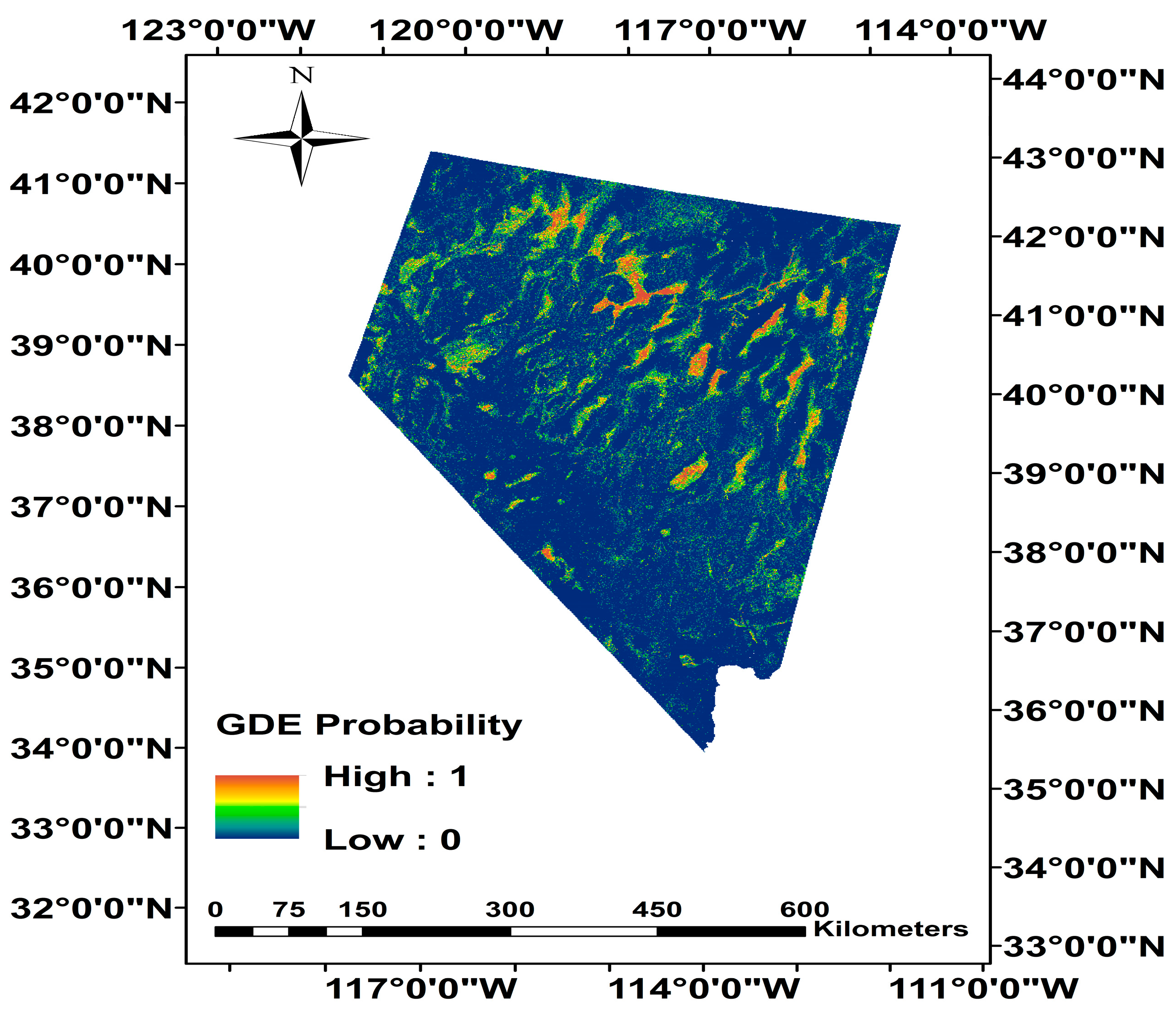
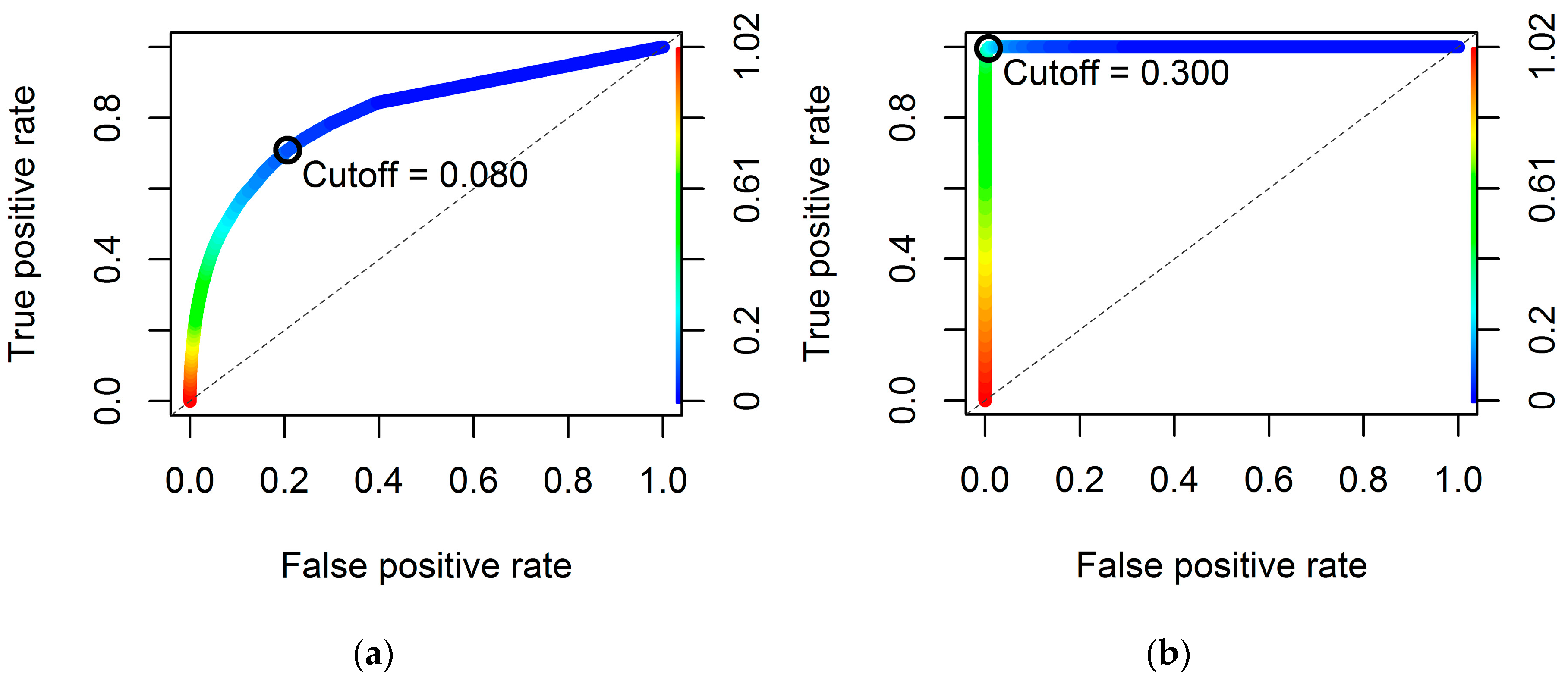
The random forest algorithm was able to obtain high values of sensitivity (sensitivity = 0.71) while maintaining a small false positive rate (FPR = 1-specificity = 0.21) which is characteristic of accurate classifiers. These results suggest that an ensemble of trees (RF) results in a better predictive model as compared to a single classification tree, although some of the threshold-dependent criteria do not show RF to be superior to CT. Ultimately, the main objective of this research is to create a versatile map that can be used in a wide variety of management applications and, therefore, continuous probability maps are preferred, not only allowing threshold selection to be matched with map use but also letting users evaluate probabilistic (threshold-independent) accuracy measures such as the map’s discrimination and calibration [41]. The resulting probability map, derived using RF on the entire data set, is shown in Figure 3.
Using the probability value that minimizes the misclassification rate of the model as a threshold, the average WTD and AI values were calculated for all the pixels classified as GDEs (19.2 m and 0.20 respectively) and for pixels classified as NON-GDEs (28.0 m and 0.23, respectively). There is a significant difference between the average WTD of GDEs and NON-GDEs of about 9 m whereas the average value of AI is very similar for both GDEs and NON-GDEs. These results suggest that NON-GDEs are associated with deeper water tables than GDEs. On the other hand, the average GDE probabilities with shallow (≤10 m), intermediate (10–30 m), and deep WTDs (>30 m) are 0.50, 0.08, and 0.02, respectively. These results highlight the fact that as the WTD increases the probability of an ecosystem to being groundwater dependent decreases non-linearly. In the case of AI, the average GDE probability values are 0.10 for arid climate, 0.08 for semi-arid climate, and 0.0 for dry sub-humid and humid conditions. This means that the more arid environments are associated with higher probabilities of the ecosystems to being groundwater dependent. Findings from this study agree with previous research on GDEs. Higher density of groundwater dependent vegetation is associated with arid and semi-arid locations where groundwater is available [79,80,81]. Regarding the interactions between predictor variables, there does not seem to be any relationship between WTD and AI. The average AI values under shallow, intermediate, and deep WTDs are close (1.19, 1.55, and 1.54, respectively), consistent with the very low correlation calculated between WTD and AI. The same behavior is observed when calculating average WTD values for arid, semi-arid, dry sub-humid, and humid conditions (2.13 m, 2.21 m, 2.38 m, and 2.35 m, respectively). This agrees with recent findings [53] where a shallow WTD was observed in both arid and humid climates. Shallow WTDs are found in humid climates such as Eastern North America, but they are also found in the arid valleys, such as those found in the Southwestern United States. According to [53], climate is the primary driver of groundwater depth for regional scales. However, at more local scales (such as within Nevada) the topography is the primary driver.

Random Forest Performance Summary

Although the main objective of this paper is to provide a continuous probability map that depicts the likelihood of an ecosystem to be groundwater dependent, the selection of conservation areas for the protection of GDEs relies on the availability of maps that define potential GDEs according to particular classification criteria. The process of translating probability estimates to a binary classification map (GDE/NON-GDE) requires the choice of a threshold. If the predicted probability value is greater than or equal to the cutoff, the pixel can be classified deterministically as GDE. Otherwise, the pixel is classified as NON-GDE. For different values of the cutoff, there are varying percentages of pixels that are classified as GDEs. For this reason, a summary of the random forest model performance measures for possible cutoff values using all the available data (both training and testing, 286,291 points) is presented in Table 3 and Table 4.
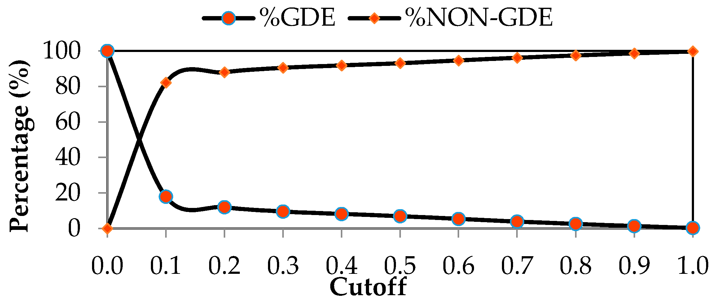
It is important to note that the most significant change from one threshold value to another occurs in the lower cutoff values (0.0 to 0.1) (See Figure 4). In this range, the percentage of pixels that are classified as GDEs goes from 100% (cutoff equal to 0.0) to 18% (cutoff equal to 0.1). The rate of change in the percentage of pixels classified as GDEs becomes smaller after a cutoff value of 0.2 with a total difference of only 12% in the pixels classified as GDEs from a threshold value equal to 0.2 to a value equal to 1.0. This means that for the selection of the cutoff value in the definition of GDEs, it is more important to pay close attention to this inflection point in the %GDE curve rather than in the higher threshold values where a different selection would not have a substantial impact on the amount of pixels classified as GDEs.
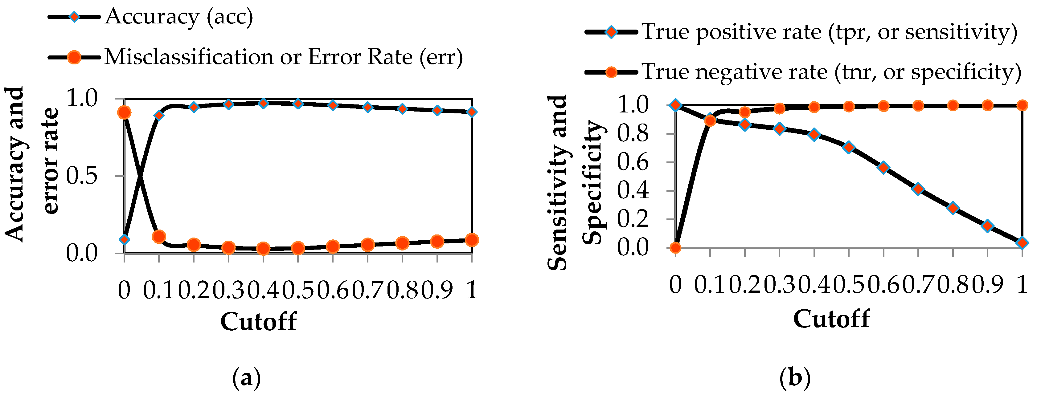
As expected, as accuracy and specificity increase, error rate and sensitivity decrease (Figure 5.) Similar to the behavior of Figure 4, for threshold values greater than 0.2, the changes in accuracy, error rate, and specificity with an increase in the cutoff value become very small.
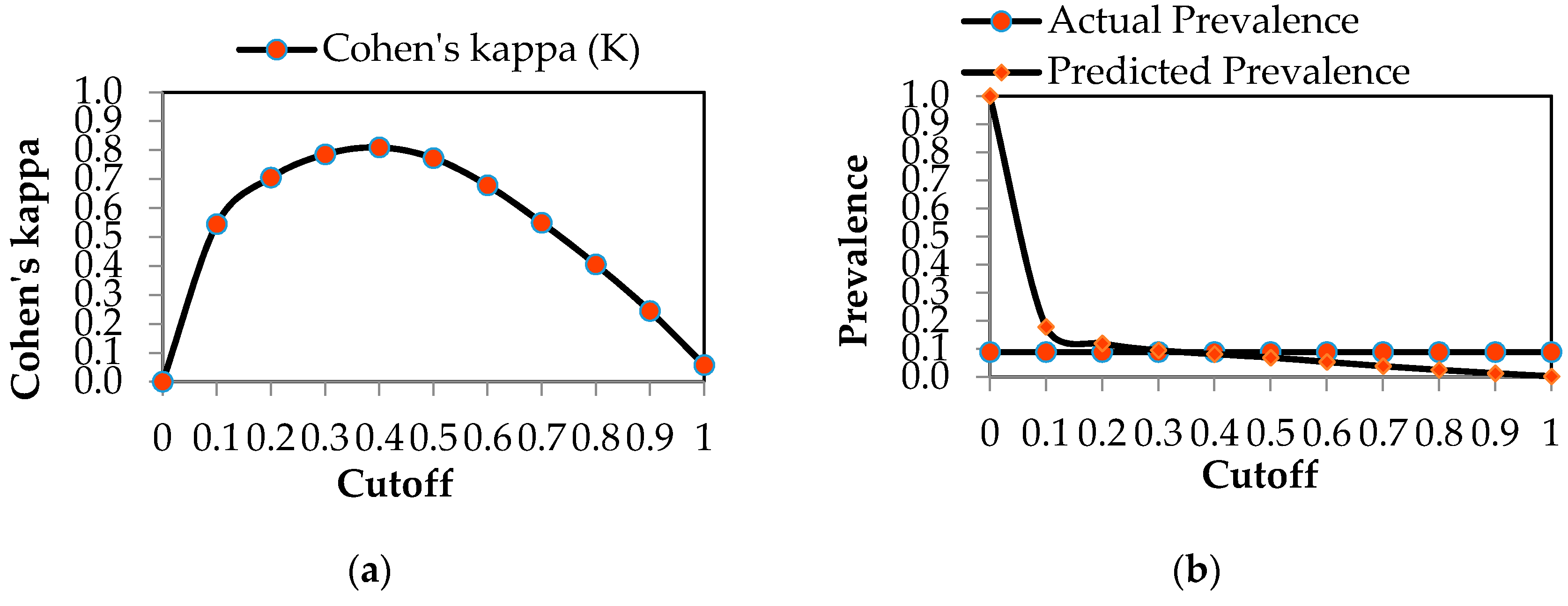
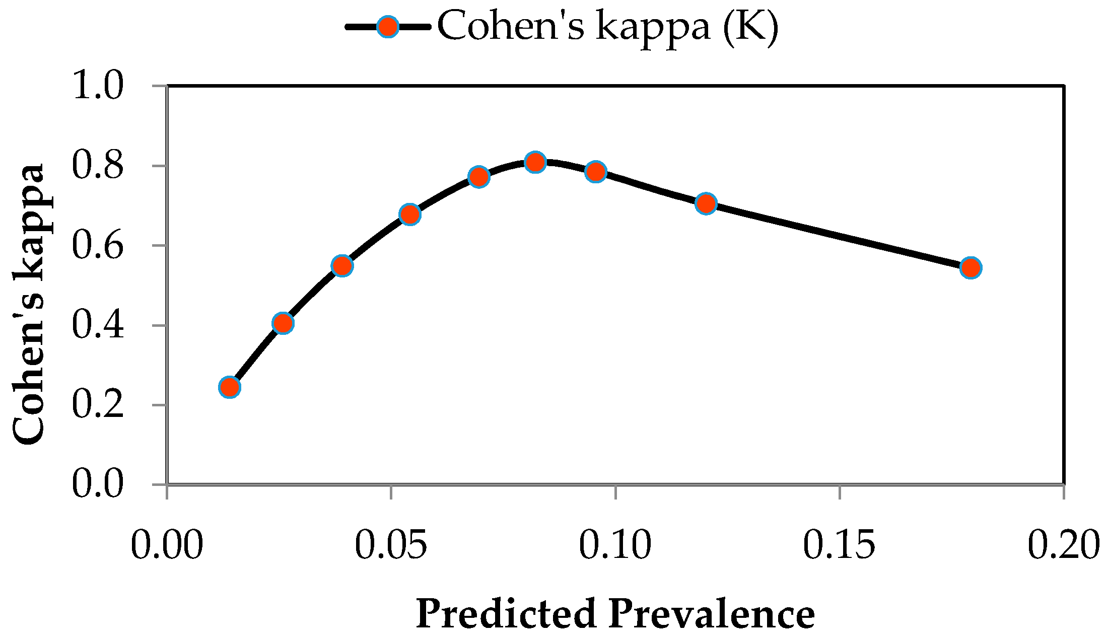
If kappa is plotted against binary classification cutoff value (Figure 6a) it is possible to visualize the sensitivity of kappa statistic to the selection of the threshold. The maximum kappa value of 0.81 is obtained with a threshold value of 0.4 which is equal to the threshold value that would be selected if the actual prevalence curve intersects the predicted prevalence curve (Figure 6b). Even though Cohen’s kappa provides a simple, effective and standardized statistic for assessment and comparison of classifiers, kappa has been found to be affected by prevalence. As it is shown in Figure 7, kappa is maximized approximately where predicted prevalence is equal to the actual prevalence of 0.09.

4. Discussion

This study was able to develop a methodology to create a groundwater dependence probability map. This product can be used in a variety of resource management applications, ranging from preventive or proactive management approaches (e.g., developing policies that focus in the protection of GDEs that have important values for groundwater users and ecosystem managers) to reactive management techniques (e.g., to mitigate and reverse the loss of groundwater dependent vegetation caused by increased groundwater pumping). Providing users with the continuous probability map, instead of a binary classification map, allows selection of the threshold value that can be matched to the interests of the main stakeholders and the map’s final use. The evaluation of different criteria for the selection of the cutoff probability should be based on the potential range of interests of groundwater stakeholders. This assessment could be used for systematic GDE conservation planning. In other words, land ecosystems dependent on groundwater within a given region can be protected by placing constraints in activities or land uses that may pose a threat. The scenarios presented here can be considered as different means to articulate the GDE conservation planning problem [21].
A cutoff probability can be selected using several approaches. The simplest and most commonly used method is to select a cutoff probability equal to 0.5. Using this value, an instance or pixel is classified as groundwater dependent if its probability of presence is greater or equal than 0.5. Otherwise, we classify the pixel as NON-GDE. However, selection of this cutoff probability does not always result in the highest prediction accuracy. In general, a threshold value of 0.5 is valid when the cost of misclassification is equal for both classes, which means that the benefit of making a correct classification is not higher for one class than the other. An important disadvantage of using this cutoff value is the fact that unequal class distributions in the response variable can greatly affect the probabilities that are calculated using the classifiers. The obtained probability surface map is often biased toward the class with the predominant size [21]. For this study, it is clear that class sizes are unequal for the response variable (9% of pixels are GDE and 91% are NON-GDE) and it is expected that the predicted probability values will be biased toward zero and few will exceed 0.5. Thus, we do not generally recommend the use of a threshold of 0.5 for any applications involving the use of a continuous GDE probability map.
Another criterion that has become popular for selection of thresholds involves ROC plots. Since the upper left corner of the ROC curve is considered to represent the “best” model, the cutoff value that is able to minimize the distance between the ROC curve and this point is considered as the “optimal cutoff probability”. This threshold minimizes (1-sensitivity)2 + (specificity-1)2. Figure 8 shows the ROC plots obtained for the independent test set (a) and the training test set (b) in the implementation of the random forest algorithm. The test set, for example, yields an optimal cutoff probability of 0.08.
Although this criterion is visually intuitive, its quadratic dependence on sensitivity and specificity need not coincide with the interests of groundwater stakeholders. Another alternative for threshold selection is the maximization of the sum of sensitivity and specificity. That is equivalent to maximizing the proportion of correctly predicted observations in conjunction with the proportion of correctly predicted negative observations. However, Manel, et al found that this criterion applied in the problem of mapping species distribution could result in the distribution of rare species being overestimated [75]. In this study, this would mean a bias toward overestimating the number of pixels classified as GDEs compared with the actual prevalence. The choice of threshold can also be optimized based on particular management applications. In other words, based on user specified accuracy values, a cutoff probability that will meet a particular management goal can be chosen. For instance, if the objective is to limit the search window for developing a field based GDEs inventory or a sampling effort, it is critical that the survey takes into account all of the pixels that could potentially be groundwater dependent. From this perspective, the emphasis needs to be placed in meeting a predetermined sensitivity that is able to maximize the number of true positives. Therefore, if the users involved in the decision determine that it is inadmissible to miss more than 2% of the GDE pixels, a sensitivity of 0.98 will be required.
On the other hand, if a preventive management approach is attempted, the threshold selection process could be based on required specificity. This criterion has been defined as the threshold that will provide the highest possible sensitivity, while still meeting a predetermined specificity [41]. With this criterion, the user can define the maximum percentage that is allowed for misclassification of NON-GDEs. In this case, a conservation planner might prefer to ensure that only highly suitable areas are selected as GDEs for preventative management based on the limited resources available for conservation.
On the contrary, if a reactive management approach is necessary, a less stringent threshold probability would be required and, therefore, a cutoff value based on a required sensitivity is suggested. This criterion will yield the highest possible specificity while still meeting a predetermined sensitivity. In other words, the user has the ability to define the maximum acceptable percentage of misclassified GDEs, therefore requiring a specific sensitivity value. This approach is useful in cases where it is most important that the area classified as GDE does not miss actual GDEs. This is particularly the case for areas where poor control over groundwater resource extraction has already had negative impacts on GDEs. The importance of reactive actions in these areas could mean the difference between ecosystems irreversibly losing their ecological function or ecosystems recovering their structure and function after restrictions are placed on the volume and distribution of groundwater withdrawal and rigorous constraints are placed over the generation of groundwater contaminant loads [82].
Another way of approaching the selection of the threshold value can take into account the surface water shortage in a given region. Three scenarios are defined that include no surface water shortage, moderate shortage, and high shortage (See Table 5).
For a sustainable development of water resources, both the satisfaction of basic human needs and the conservation of ecosystems are called for. However, when drought conditions occur, the urgencies of different stakeholders could be conflicting and a priority stakeholder should be established. If there is no surface water shortage, the priority could be placed in the safeguarding and maintenance of ecosystems since water requirements for human activities can be met with surface water supplies. From this perspective, priority would be given to stakeholders that are focused in ecological conservation, such as local water resource, land planning, and environmental protection agencies (WB). For this purpose, the recommendation is to set a predetermined sensitivity as the criterion for threshold selection. On the other hand, if there is a moderate surface water shortage, equal importance should be given to the safeguarding of ecosystems and the sufficient allocation of water for human use. In this case, it is important that the predicted prevalence (threshold-dependent) is able to represent the actual prevalence (independent of threshold) which means that the management objective will be focused in providing unbiased estimates of ecosystems prevalence. Finally, if there is a high surface water shortage, meeting basic water needs for humans might be essential before considering ecological water needs. Therefore, the stakeholders that will have priority may include the rural, urban, and industrial sectors. Therefore, threshold selection criteria could be based in the achievement of a required specificity to focus on the areas most likely to contain GDEs.

5. Conclusions

The probability of an ecosystem to being reliant on groundwater is defined here based on a random forest classifier model. When given a set of relevant characteristics for a particular pixel, namely WTD and AI, along with training data, RF enables one to answer whether that point is likely dependent on groundwater. Shallow water tables occur in areas where ecosystem groundwater dependence is expected. Additionally, water level is the most important limiting factor for groundwater availability and use by plants. Therefore, pixels with shallow water tables have higher probability estimates to be GDEs than pixels with deep water tables. This means that an ecosystem with a greater access to groundwater is expected to develop greater dependency on this resource. On the other hand, AI quantifies the precipitation availability and atmospheric water demand, which means that higher AI values represent more humidity and low AI values represent high aridity and consequently less availability of surface water to supply ecosystem water requirements. For this reason, pixels with low AI values have higher GDE probability than pixels with high AI values.
Based on the AUC value, random forest classification provides a superior capability, when compared to a single classification tree, to generate probability estimates. Considering a threshold value that minimizes the misclassification rate for each model, a random forest is also proven to be more accurate than classification trees for both the training and the testing data. For the training data, all of the performance measures considered (accuracy, sensitivity, specificity, kappa) are higher for the random forest than for classification trees. Regarding test data, classification trees result in higher accuracy, specificity, and kappa values. Higher values for CT of accuracy and kappa highlight the fact that both measures are very affected by low prevalence, which is a characteristic of the data used in this study. Because of this low prevalence, the classification trees try to maximize accuracy by assigning the NON-GDE class to the majority of pixels. In consequence, a high specificity is obtained and the resulting model is biased towards the NON-GDE class. The kappa statistic may not be adequate for accuracy assessment where prevalence is low.
The outcome of RF modeling is a GDE probability map that can be used to classify cases into one of two groups, GDE or NON-GDE, which results in a binary classification problem that arises when data needs to be separated into two distinct classes using some “optimal” method. This is achieved by selecting a cutoff value. The choice of the cutoff probability value has important consequences on model accuracy and for the overall proportion of locations where the ecosystems are found to be groundwater dependent by changing the frequencies of the two possible misclassification errors, false positives versus false negatives. Different criteria for choosing a cutoff value are possible, which can be related to management priorities and the relative importance of avoiding the two types of errors.

Acknowledgments

The authors gratefully acknowledge support from NOAA awards NA11SEC4810004, NA12OAR4310084, NA15OAR4310080; PSC-CUNY Award 68346-00 46; CUNY CIRG Award 2207; and the USAID IPM Innovation Lab award “Participatory Biodiversity and Climate Change Assessment for Integrated Pest Management in the Annapurna-Chitwan Landscape, Nepal”. All statements made are the views of the authors and not the opinions of the funding agency or the U.S. government.

Author Contributions

Isabel C. Pérez Hoyos collected and analyzed the data, interpreted results, and wrote the manuscript. Nir Y. Krakauer and Reza Khanbilvardi were responsible for supervising the study, providing key input for the methods and materials used in this research, and revising the manuscript.

Conflicts of Interest

The authors declare no conflict of interest.

References

  1. Glasser, S.; Gauthier-Warinner, J.; Keely, J.; Gurrieri, J.; Tucci, P.; Summers, P.; Wireman, M.; McCormack, K. Technical Guide to Managing Ground Water Resources; United States Department of Agriculture: Washington, DC, USA, 2007.
  2. Eamus, D. Identifying Groundwater Dependent Ecosystems: A Guide for Land and Water Managers; Australian Government, Land and Water Australia: Sydney, Australia, 2009.
  3. Contreras, S.; Jobbágy, E.G.; Villagra, P.E.; Nosetto, M.D.; Puigdefábregas, J. Remote sensing estimates of supplementary water consumption by arid ecosystems of central Argentina. J. Hydrol. 2011, 397, 10–22. [Google Scholar] [CrossRef]
  4. Mathie, A.M.; Welborn, T.L.; Susong, D.D.; Tumbusch, M.L. Phreatophytic Land-Cover Map of the Northern and Central Great Basin Ecoregion: California, Idaho, Nevada, Utah, Oregon, and Wyoming; U.S. Geological Survey: Reston, VA, USA, 2011.
  5. Lawford, R.; Strauch, A.; Toll, D.; Fekete, B.; Cripe, D. Earth observations for global water security. Curr. Opin. Environ. Sustain. 2013, 5, 633–643. [Google Scholar] [CrossRef]
  6. Münch, Z.; Conrad, J. Remote sensing and GIS based determination of groundwater dependent ecosystems in the Western Cape, South Africa. Hydrogeol. J. 2006, 15, 19–28. [Google Scholar] [CrossRef]
  7. Merz, S.K. Atlas of Groundwater Dependent Ecosystems (GDE Atlas); Australian Government, National Water Commission: Melbourne, Australia, 2012.
  8. Colvin, C.; Le Maitre, D.; Hughes, S. Assessing Terrestrial Groundwater Dependent Ecosystems in South Africa; Water Research Commission: Pretoria, South Africa, 2003. [Google Scholar]
  9. Gow, L.; Brodie, R.S.; Green, R.; Punthakey, J.; Woolley, D.; Redpath, P.; Bradburn, A. Identification and monitoring GDEs using MODIS time series: Hat Head National Park—A case study. In Groundwater 2010: The Challenge of Sustainable Management; National Convention Centre: Canberra, Australia, 2010. [Google Scholar]
  10. Werstak, C.E.; Housman, I.; Maus, P.; Fisk, H.; Gurrieri, J.; Carlson, C.P.; Johnston, B.C.; Stratton, B.; Hurja, J.C. Groundwater-Dependent Ecosystem Inventory Using Remote Sensing, RSAC-10011-RPT1; Remote Sensing Applications Center: Salt Lake City, UT, USA, 2012. [Google Scholar]
  11. Heidel, B.; Rodemaker, E. Inventory of Peatland Systems in the Beartooth Mountains, Shoshone National Forest; Environmental Protection Agency: Laramie, WY, USA, 2008.
  12. Brown, J.; Wyers, A.; Bach, L.; Aldous, A. Groundwater-Dependent Biodiversity and Associated Threats: A Statewide Screening Methodology and Spatial Assessment of Oregon; The Nature Conservancy: Arlington, VA, USA, 2009. [Google Scholar]
  13. Howard, J.; Merrifield, M. Mapping groundwater dependent ecosystems in California. PLoS ONE 2010, 5. [Google Scholar] [CrossRef] [PubMed]
  14. Brown, J.; Bach, L.; Aldous, A.; Wyers, A.; DeGagné, J. Groundwater-dependent ecosystems in Oregon: An assessment of their distribution and associated threats. Front. Ecol. Environ. 2011, 9, 97–102. [Google Scholar] [CrossRef]
  15. Elith, J.; Leathwick, J.R. Species Distribution Models: Ecological Explanation and Prediction across Space and Time. Annu. Rev. Ecol. Evol. Syst. 2009, 40, 677–697. [Google Scholar] [CrossRef]
  16. Manel, S.; Dias, J.M.; Buckton, S.T.; Ormerod, S.J. Alternative methods for predicting species distribution: An illustration with Himilayan river birds. J. Appl. Ecol. 1999, 36, 734–747. [Google Scholar] [CrossRef]
  17. Kath, J.; Le Brocque, A.; Leyer, I.; Mosner, E. Hydrological and land use determinants of Eucalyptus camaldulensis occurrence in floodplain wetlands. Austral Ecol. 2014, 39, 643–655. [Google Scholar] [CrossRef]
  18. Leyer, I. Predicting plant species’ responses to river regulation: The role of water level fluctuations. J. Appl. Ecol. 2005, 42, 239–250. [Google Scholar] [CrossRef]
  19. Kath, J.; Powell, S.; Reardon-Smith, K.; El Sawah, S.; Jakeman, A.J.; Croke, B.F.W.; Dyer, F.J. Groundwater salinization intensifies drought impacts in forests and reduces refuge capacity. J. Appl. Ecol. 2015, 52, 1116–1125. [Google Scholar] [CrossRef]
  20. Cunningham, S.C.; Thomson, J.R.; Mac Nally, R.; Read, J.; Baker, P.J. Groundwater change forecasts widespread forest dieback across an extensive floodplain system. Freshw. Biol. 2011, 56, 1494–1508. [Google Scholar] [CrossRef]
  21. Wilson, K.A.; Westphal, M.I.; Possingham, H.P.; Elith, J. Sensitivity of conservation planning to different approaches to using predicted species distribution data. Biol. Conserv. 2005, 122, 99–112. [Google Scholar] [CrossRef]
  22. Pérez Hoyos, I.; Krakauer, N.; Khanbilvardi, R.; Armstrong, R. A review of advances in the identification and characterization of groundwater dependent ecosystems using geospatial technologies. Geosciences 2016, 6. [Google Scholar] [CrossRef]
  23. Batelaan, O.; Witte, J.P.M. Ecohydrology and groundwater dependent terrestrial ecosystems. In Proceedings of the 28th Annual Conference of the International Association of Hydrogeologists (Irish Group), Tullamore, Ireland, 22–23 April 2008; pp. 1–8.
  24. Rodriguez-Iturbe, I. Ecohydrology: A hydrologic perspective of climate-soil-vegetation dynamics. Water Resour. Res. 2000, 36, 3–9. [Google Scholar] [CrossRef]
  25. Froend, R.; Loomes, R.; Horwitz, P.; Bertuch, M.; Storey, A.; Bamford, M. Study of Ecological Water Requirements on the Gnangara and Jandakot Mounds under Section 46 of the Environmental Protection Act Task 2: Determination of Ecological Water Requirements; Center for Ecosystem Management: Perth, Australia, 2004. [Google Scholar]
  26. Kløve, B.; Ala-aho, P.; Bertrand, G.; Boukalova, Z.; Ertürk, A.; Goldscheider, N.; Ilmonen, J.; Karakaya, N.; Kupfersberger, H.; Kvoerner, J.; et al. Groundwater dependent ecosystems. Part I: Hydroecological status and trends. Environ. Sci. Policy 2011, 14, 770–781. [Google Scholar] [CrossRef]
  27. Laio, F.; Tamea, S.; Ridolfi, L.; D’Odorico, P.; Rodriguez-Iturbe, I. Ecohydrology of groundwater-dependent ecosystems: 1. Stochastic water table dynamics. Water Resour. Res. 2009, 45. [Google Scholar] [CrossRef]
  28. Guswa, A.J.; Celia, M.; Rodriguez-Iturbe, I. Models of soil moisture dynamics in ecohydrology: A comparative study. Water Resour. Res. 2002, 38. [Google Scholar] [CrossRef]
  29. Guswa, A.J. Soil-moisture limits on plant uptake: An upscaled relationship for water-limited ecosystems. Adv. Water Resour. 2005, 28, 543–552. [Google Scholar] [CrossRef]
  30. Laio, F. A vertically extended stochastic model of soil moisture in the root zone. Water Resour. Res. 2006, 42, 1–10. [Google Scholar] [CrossRef]
  31. Laio, F.; Porporato, A.; Fernandez-Illescas, C.; Rodriguez-Iturbe, I. Plants in water-controlled ecosystems: Active role in hydrologic processes and response to water stress. Adv. Water Resour. 2001, 24, 745–762. [Google Scholar] [CrossRef]
  32. Porporato, A.; D’Odorico, P.; Laio, F.; Ridolfi, L.; Rodriguez-Iturbe, I. Ecohydrology of water-controlled ecosystems. Adv. Water Resour. 2002, 25, 1335–1348. [Google Scholar] [CrossRef]
  33. Rodríguez-Iturbe, I.; Porporato, A. Ecohydrology of Water-Controlled Ecosystems; Soil Moisture and Plant Dynamics; Cambridge University Press: Cambridge, UK, 2004. [Google Scholar]
  34. Rodriguez-Iturbe, I.; Porporato, A.; Ridolfi, L.; Isham, V.; Coxi, D.R. Probabilistic modelling of water balance at a point: The role of climate, soil and vegetation. Proc. R. Soc. Lond. A Math. Phys. Eng. Sci. 1999, 455, 3789–3805. [Google Scholar] [CrossRef]
  35. Tamea, S.; Laio, F.; Ridolfi, L.; D’Odorico, P.; Rodriguez-Iturbe, I. Ecohydrology of groundwater-dependent ecosystems: 2. Stochastic soil moisture dynamics. Water Resour. Res. 2009, 45. [Google Scholar] [CrossRef]
  36. D’odorico, P.; Laio, F.; Porporato, A.; Ridolfi, L.; Rinaldo, A.; Rodriguez, I. Ecohydrology of Terrestrial Ecosystems. Bioscience 2010, 60, 898–907. [Google Scholar] [CrossRef]
  37. Asbjornsen, H.; Goldsmith, G.R.; Alvarado-Barrientos, M.S.; Rebel, K.; Van Osch, F.P.; Rietkerk, M.; Chen, J.; Gotsch, S.; Tobón, C.; Geissert, D.R.; et al. Ecohydrological advances and applications in plant-water relations research: A review. J. Plant Ecol. 2011, 4, 3–22. [Google Scholar] [CrossRef]
  38. Sinclair Knight Merz Pty. Ltd. Environmental Water Requirements to Maintain Groundwater Dependent Ecosystems; Commonwealth of Australia: Canberra, Australia, 2001.
  39. Richardson, S.; Irvine, E.; Froend, R.; Boon, P.; Barber, S.; Bonneville, B. Australian Groundwater Dependent Ecosystems Toolbox Part 1: Assessment Framework; National Water Commission: Canberra, Australia, 2011.
  40. Dresel, P.E.; Clark, R.; Cheng, X.; Reid, M.; Terry, A.; Fawcett, J.; Cochrane, D. Mapping Terrestrial Groundwater Dependent Ecosystems: Method Development and Example Output; Department of Primary Industries: Melbourne, Australia, 2010.
  41. Freeman, E.A.; Moisen, G.G. A comparison of the performance of threshold criteria for binary classification in terms of predicted prevalence and kappa. Ecol. Model. 2008, 217, 48–58. [Google Scholar] [CrossRef]
  42. Perez Hoyos, I.C.; Krakauer, N.; Khanbilvardi, R. Random Forest for Identification and Characterization of Groundwater Dependent Ecosystems. WIT Trans. Ecol. Environ. 2015, 196, 89–100. [Google Scholar]
  43. Weisberg, P. Nevada Vegetation Overview. Available online: http://www.onlinenevada.org/articles/nevada-vegetation-overview (accessed on 14 November 2015).
  44. Pritchett, D.; Manning, S.J. Response of an Intermountain Groundwater-Dependent Ecosystem to Water Table Drawdown. West. N. Am. Nat. 2012, 72, 48–59. [Google Scholar] [CrossRef]
  45. Pritchett, D.W.; Manning, S.J. Effects of Fire and Groundwater Extraction on Alkali Meadow Habitat in Owens Valley, California. Madroño 2009, 56, 89–98. [Google Scholar] [CrossRef]
  46. Aldous, A.R.; Bach, L.B. Hydro-ecology of groundwater-dependent ecosystems: Applying basic science to groundwater management. Hydrol. Sci. J. 2014, 59, 530–544. [Google Scholar] [CrossRef]
  47. Roberts, J.J.; Best, B.D.; Dunn, D.C.; Treml, E.A.; Halpin, P.N. Environmental Modelling & Software Marine Geospatial Ecology Tools: An integrated framework for ecological geoprocessing with ArcGIS, Python, R, MATLAB, and C++. Environ. Model. Softw. 2010, 25, 1197–1207. [Google Scholar]
  48. Threneau, T.; Atkinson, B.; Ripley, B. Package “rpart”: Recursive Partitioning and Regression Trees; CRANR Project: Rochester, NY, USA, 2015; pp. 1–34. [Google Scholar]
  49. Liaw, A.; Wiener, M. Classification and Regression by Random Forest. R News 2002, 2, 18–22. [Google Scholar]
  50. R Foundation for Statistical Computing. R Development Core Team: A Language and Environment for Statistical Computing; R Core Team: Vienna, Austria, 2011. [Google Scholar]
  51. ESRI ArcGIS Desktop: Release 10.2. Environmental Systems Research Institute: Redlands, USA, 2013.
  52. Middleton, N.; Thomas, D. World Atlas of Desertification, 2nd ed.; United Nations Environment Program, Ed.; Routledge: London, UK, 1997. [Google Scholar]
  53. Fan, Y.; Li, H.; Miguez-Macho, G. Global Patterns of Groundwater Table Depth. Science 2013, 339, 940–943. [Google Scholar] [CrossRef] [PubMed]
  54. Perez Hoyos, I.C.; Krakauer, N.; Khanbilvardi, R. Prediction of water table depth from geospatial and remote sensing data using random forests. WIT Int. J. Sustain. Dev. Plan. 2016. submitted. [Google Scholar]
  55. Zomer, R.J.; Trabucco, A.; Bossio, D.A.; Verchot, L.V. Climate change mitigation: A spatial analysis of global land suitability for clean development mechanism afforestation and reforestation. Agric. Ecosyst. Environ. 2008, 126, 67–80. [Google Scholar] [CrossRef]
  56. Zomer, J.R.; Bossio, A.D.; Trabucco, A.; Yuanjie, L.; Gupta, C.D.; Singh, P.V. Trees and Water: Smallholder Agroforestry on Irrigated Lands in Northern India; International Water Management Institute: Colombo, Sri Lanka, 2007. [Google Scholar]
  57. Piper, M.E.; Loh, W.-Y.; Smith, S.S.; Japuntich, S.J.; Baker, T.B. Using decision tree analysis to identify risk factors for relapse to smoking. Subst. Use Misuse 2011, 46, 492–510. [Google Scholar] [CrossRef] [PubMed]
  58. Buto, S.G.; Sweetkind, D.S. 1:1,000,000-Scale Hydrographic Areas and Flow Systems for the Great Basin Carbonate and Alluvial Aquifer System of Nevada, Utah, and Parts of Adjacent States; U.S. Geological Survey: Reston, VA, USA, 2011.
  59. Batelaan, O.; De Smedt, F.; Triest, L. Regional groundwater discharge: Phreatophyte mapping, groundwater modelling and impact analysis of land-use change. J. Hydrol. 2003, 275, 86–108. [Google Scholar] [CrossRef]
  60. Tóth, J. Groundwater Discharge: A Common Generator of Diverse Geologic and Morphologic Phenomena. Int. Assoc. Sci. Hydrol. Bull. 1971, 16, 7–24. [Google Scholar] [CrossRef]
  61. Klijn, F.; Witte, J.P.M. Eco-hydrology: Groundwater flow and site factors in plant ecology. Hydrogeol. J. 1999, 7, 65–77. [Google Scholar] [CrossRef]
  62. Rosenberry, D.O.; Striegl, R.G.; Hudson, D.C. Plants as indicatosr of focused ground water discharge to a Northern Minnesota Lake. Ground Water 2000, 38, 296–303. [Google Scholar] [CrossRef]
  63. Laczniak, R.J.; Moreo, M.T.; Smith, J.L.; Harper, D.P.; Welborn, T.L. Potential Areas of Ground-Water Discharge in the Basin and Range Carbonate-Rock Aquifer System, White Pine County, Nevada, and Adjacent Parts of Nevada and Utah; U.S. Geological Survey: Reston, VA, USA, 2007.
  64. Provost, F.; Domingos, P. Well-Trained PETs: Improving Probability Estimation Trees; New York University: New York, NY, USA, 2000. [Google Scholar]
  65. Prasad, A.M.; Iverson, L.R.; Liaw, A. Newer Classification and Regression Tree Techniques: Bagging and Random Forests for Ecological Prediction. Ecosystems 2006, 9, 181–199. [Google Scholar] [CrossRef]
  66. Waljee, A.K.; Higgins, P.D.R.; Singal, A.G. A primer on predictive models. Clin. Transl. Gastroenterol. 2014, 5. [Google Scholar] [CrossRef] [PubMed]
  67. Moons, K.G.M.; Royston, P.; Vergouwe, Y.; Grobbee, D.E.; Altman, D.G. Prognosis and prognostic research: What, why, and how? BMJ 2009, 338. [Google Scholar] [CrossRef] [PubMed]
  68. Chawla, N.; Cieslak, D. Evaluating probability estimates from decision trees. Am. Assoc. Artif. Intell. 2006, 23, 18–23. [Google Scholar]
  69. Provost, F.; Domingos, P. Tree Induction for Probability-based Ranking. Mach. Learn. 2003, 52, 199–215. [Google Scholar] [CrossRef]
  70. Zadrozny, B.; Elkan, C. Learning and making decisions when costs and probabilities are both unknown. In Proceedings of the Seventh International Conference on Knowledge Discovery and Data Mining, San Diego, CA, USA, 21–24 August 2001; pp. 204–213.
  71. Moisen, G.G.; Freeman, E.A.; Blackard, J.A.; Frescino, T.S.; Zimmermann, N.E.; Edwards, T.C. Predicting tree species presence and basal area in Utah: A comparison of stochastic gradient boosting, generalized additive models, and tree-based methods. Ecol. Model. 2006, 199, 176–187. [Google Scholar] [CrossRef]
  72. Fawcett, T. An introduction to ROC analysis. Pattern Recognit. Lett. 2006, 27, 861–874. [Google Scholar] [CrossRef]
  73. Swets, J.A. Measuring the Accuracy of Diagnostic Systems. Science 1988, 240, 1285–1293. [Google Scholar] [CrossRef] [PubMed]
  74. Fielding, A.H.; Bell, J.F. A review of methods for the assessment of prediction errors in conservation presence/absence models. Environ. Conserv. 1997, 24, 38–49. [Google Scholar] [CrossRef]
  75. Manel, S.; Ceri Williams, H.; Ormerod, S.J. Evaluating presence-absence models in ecology: The need to account for prevalence. J. Appl. Ecol. 2001, 38, 921–931. [Google Scholar] [CrossRef]
  76. Krakauer, N.Y.; Grossberg, M.D.; Gladkova, I.; Aizenman, H. Information content of seasonal forecasts in a changing climate. Adv. Meteorol. 2013, 2013. [Google Scholar] [CrossRef]
  77. Allouche, O.; Tsoar, A.; Kadmon, R. Assessing the accuracy of species distribution models: Prevalence, kappa and the true skill statistic (TSS). J. Appl. Ecol. 2006, 43, 1223–1232. [Google Scholar] [CrossRef]
  78. Viera, A.J.; Garrett, J.M. Understanding interobserver agreement: The kappa statistic. Fam. Med. 2005, 37, 360–363. [Google Scholar] [PubMed]
  79. Eamus, D.; Zolfaghar, S.; Villalobos-Vega, R.; Cleverly, J.; Huete, A. Groundwater-dependent ecosystems: Recent insights from satellite and field-based studies. Hydrol. Earth Syst. Sci. 2015, 19, 4229–4256. [Google Scholar] [CrossRef]
  80. Lv, J.; Wang, X.S.; Zhou, Y.; Qian, K.; Wan, L.; Eamus, D.; Tao, Z. Groundwater-dependent distribution of vegetation in Hailiutu River catchment, a semi-arid region in China. Ecohydrology 2013, 6, 142–149. [Google Scholar] [CrossRef]
  81. Jin, X.M.; Schaepman, M.E.; Clevers, J.G.P.W.; Su, Z.B.; Hu, G.C. Groundwater Depth and Vegetation in the Ejina Area, China. Arid Land Res. Manag. 2011, 25, 194–199. [Google Scholar] [CrossRef]
  82. Foster, S.; Koundouri, P.; Tuinhof, A.; Kemper, K.; Nanni, M.; Garduño, H. Groundwater Dependent Ecosystems: The Challenge of Balanced Assessment and Adequate Conservation; The World Bank: Washington, DC, USA, 2006. [Google Scholar]
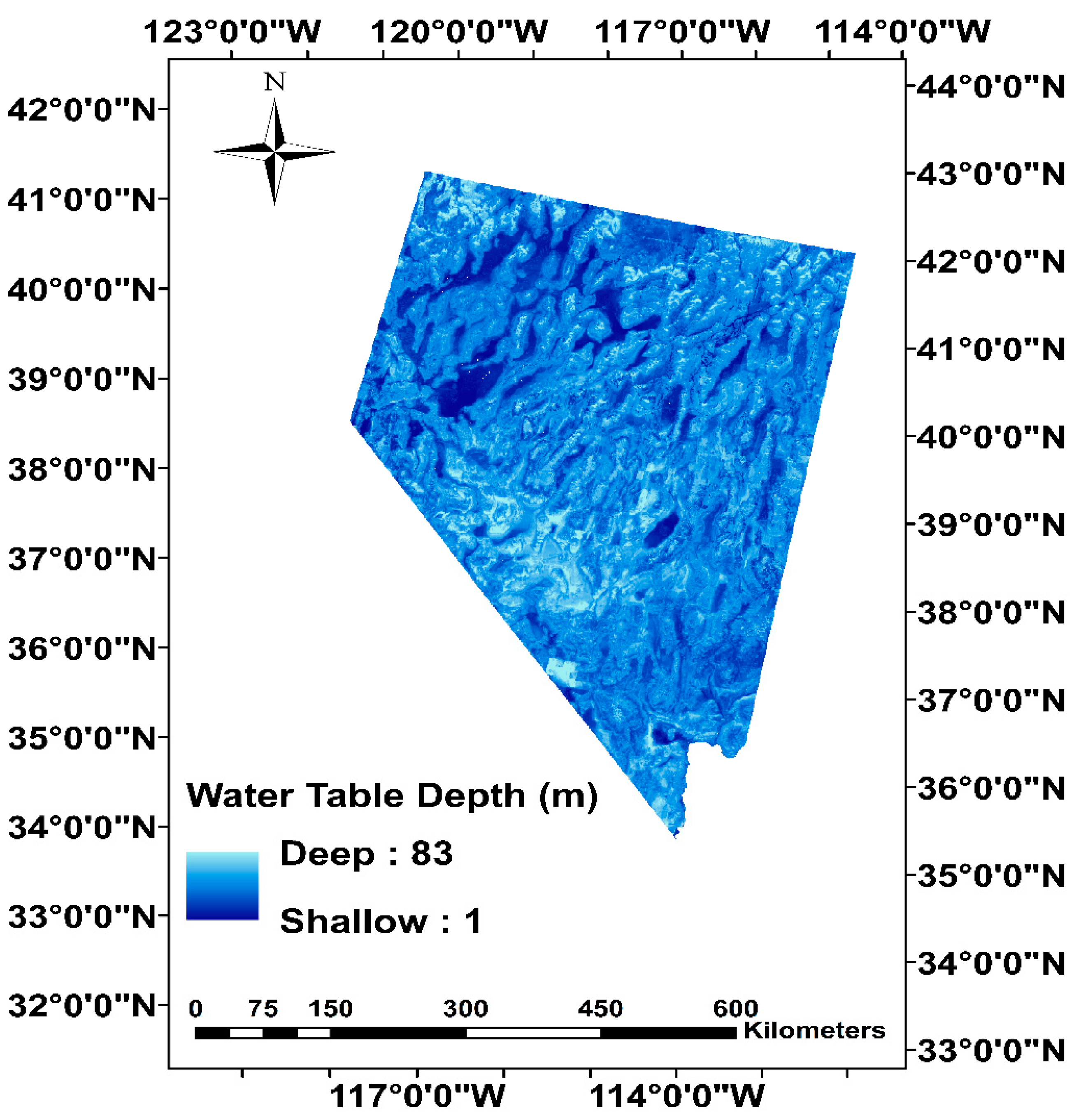
Figure 1. Water table depth map for Nevada at 1 km spatial resolution [42].
Environments 03 00009 g001
Figure 2. Aridity index map for Nevada at 1 km spatial resolution.
Environments 03 00009 g002
Figure 3. GDE Probability Estimates for Nevada obtained with random forest.
Environments 03 00009 g003
Figure 4. Percentage of GDEs and NON-GDEs predicted against binary classification cutoff values.
Environments 03 00009 g004
Figure 5. Evaluation of performance measures against binary classification cutoff value: (a) accuracy and error rate against cutoff value; and (b) sensitivity and specificity against cutoff value.
Environments 03 00009 g005
Figure 6. Evaluation of kappa and prevalence against binary classification cutoff value: (a) Cohen’s Kappa against cutoff value; (b) Actual and predicted prevalence against cutoff value.
Environments 03 00009 g006
Figure 7. Effect of predicted prevalence on the Kappa statistic.
Environments 03 00009 g007
Figure 8. ROC analysis for Random Forest. The ROC curves are color coded based on the binary classification cutoff value: (a) ROC curves for the test data; and (b) ROC curves for the training data.
Environments 03 00009 g008
Table 1. Overview of the datasets used for training of CT and RF models. Mapping scale is used for polygon features and spatial resolution is used for rasters.
DatasetsMapping Scale or Spatial ResolutionMapped FeaturesSpatial ExtentData SourceReference
Groundwater discharge as evapotranspiration1:1,000,000-scale map (Horizontal accuracy estimation of 550 m)Outer extent of preatophyte areasGreat Basin carbonate and alluvial aquifer system. Includes portions of Nevada, Utah, California, and IdahoData compiled from previous studies: BARCAS, DVRFS, Eastern Nevada, and RASA. These studies are a combination of satellite, aerial imagery, field studies, and visual verification.[58]
Potential areas of ground-water discharge1:1,000,000-scale map (Horizontal accuracy estimation of 550 m)Outer extent of preatophyte areasEastern Nevada and Western UtahUSGS and SNWA data mapped during aerial field reconnaissance. Field verification was done using GPS and visual verification.[63]
Phreatophytic Land-Cover Map of the Northern and Central Great Basin Ecoregion: California, Idaho, Nevada, Utah, Oregon, and Wyoming30 mPhreatophytic vegetationNorthern and Central Great Basin Ecoregion: California, Idaho, Nevada, Utah, Oregon, and WyomingThe data are based on the combination of land cover phreatophytic vegetation classes (obtained from Shrub Map and GAP data which are both a combiation of satellite imagery with digital elevation model derived datasets).[4]
Table 2. Comparison of classification trees (CT) and random forests (RF) modeling techniques based on accuracy measures obtained with the evaluation of testing data (30%) and training data (70%).
Accuracy MeasureTest Data (n = 85,888)Training Data (n = 200,405)
CTRFCTRF
Area under the ROC curve (AUC)0.7400.8130.7411.000
Cutoff value0.2240.0800.2240.300
Accuracy (ACC)0.8790.7860.8800.993
True positive rate (Sensitivity)0.5510.7090.5540.997
True negative rate (Specificity)0.9110.7940.9120.992
Cohen’s kappa (K)0.3840.2770.3860.957
Table 3. Percentage of pixels classified as Groundwater Dependent Ecosystems (%GDE) and percentage of pixels classified as non-groundwater dependent (%NON-GDE) for cutoff values from 0.0 to 0.4. Rows 4–8 show model performance measures for all the possible values of binary classification cutoff.
Specified Cutoff0.00.10.20.30.4
Number of pixels classified as GDEs286,29151,29434,40727,35923,500
%GDE100.017.912.09.68.2
Number of pixels classified as NON-GDEs0.000234,997251,884258,932262,791
%NON-GDE0.082.188.090.491.8
Accuracy (acc)0.0890.8920.9450.9640.970
Misclassification or Error Rate (err)0.9110.1080.0550.0360.030
True positive rate (tpr, or sensitivity)1.0000.9020.8640.8350.794
True negative rate (tnr, or specificity)0.0000.8910.9520.9770.987
Cohen’s kappa (K)0.0000.5440.7050.7850.809
Table 4. Percentage of pixels classified as Groundwater Dependent Ecosystems (%GDE) and percentage of pixels classified as non-groundwater dependent (%NON-GDE) for cutoff values from 0.5 to 1.0. Rows 4–8 show model performance measures for possible values of binary classification cutoff.
Specified Cutoff0.50.60.70.80.91.0
Number of pixels classified as GDEs19,90015,49811,16773873986848
%GDE7.05.43.92.61.40.3
Number of pixels classified as NON-GDEs266,391270,793275,124278,904282,305285,443
%NON-GDE93.094.696.197.498.699.7
Accuracy (acc)0.9670.9570.9450.9350.9240.914
Misclassification or Error Rate (err)0.0330.0430.0550.0650.0760.086
True positive rate (tpr, or sensitivity)0.7040.5620.4120.2770.1520.033
True negative rate (tnr, or specificity)0.9920.9950.9970.9991.0001.000
Cohen’s kappa (K)0.7720.6780.5490.4050.2440.058
Table 5. Guidelines for selection of binary classification cutoff value based on surface water shortage.
Surface Water ShortagePriority StakeholderThreshold Selection Criteria
No shortageEnvironment—Local water resource, land planning, and environmental protection agenciesRequired sensitivity
Moderate shortageHumans and Environment (Rural, urban, industrial, tourism sectors, and Environment)Predicted prevalence = Actual prevalence
High shortageHumans (Rural, urban, industrial, tourism sectors)Required specificity