Allometric Equations for Aboveground Biomass Estimation in Wet Miombo Forests of the Democratic Republic of the Congo Using Terrestrial LiDAR

Abstract

Accurate assessments of aboveground biomass (AGB) stocks and their changes in extensive Miombo forests are challenging due to the lack of site-specific allometric equations (AEs). Terrestrial Laser Scanning (TLS) is a non-destructive method that enables the calibration of AEs and has recently been validated by the IPCC guidelines for carbon accounting within the REDD+ framework. TLS surveys were carried out in five non-contiguous 1-ha plots in two study sites in the wet Miombo forest of Katanga, in the Democratic Republic Congo. Local wood densities (WD) were determined from wood cores taken from 619 trees on the sites. After a careful checking of Quantitative Structure Models (QSMs) output, the individual volumes of 213 trees derived from TLS data processing were converted to AGB using WD. Four AEs were calibrated using different predictors, and all presented strong performance metrics (e.g., R² ranging from 90 to 93%), low relative bias and relative individual mean error (11.73 to 16.34%). Multivariate analyses performed on plot floristic and structural data showed a strong contrast in terms of composition and structure between sites and between plots within sites. Even though the whole variability of the biome has not been sampled, we were thus able to confirm the transposability of results within the wet Miombo forests through two cross-validation approaches. The AGB predictions obtained with our best AE were also compared with AEs found in the literature. Overall, an underestimation of tree AGB varying from −35.04 to −19.97% was observed when AEs from the literature were used for predicting AGB in the Miombo of Katanga.

1. Introduction

Quantifying the role of tropical forests in the global carbon cycle and climate requires more and better ground-estimates of carbon density across the biome [1,2]. In addition, improved estimates will allow developing countries such as the Democratic Republic of the Congo (DRC) to achieve higher bids in international carbon trading schemes, such as the Reducing emissions from deforestation and forest degradation (REDD+) initiative. As most forest carbon is in the above ground biomass (AGB) of trees, attention was paid to the development of allometry equations, which are statistical models linking routine forest inventory measurements (diameter at breast height—DBH, total Height—H, and species mean wood density) to tree biomass. Traditionally, these models were calibrated using destructively sampled trees. Sampling limitation, such as the difficulty to weigh large trees or to cover all geographical and biological extant variability, is known to lead to locally important bias in estimations [3]. The AGB of the largest trees are indeed generally underestimated (by as much as 50%) even though these trees concentrate most of the carbon stock of a forest. When estimating carbon in a specific forest type, such as the Miombo forests of DRC, the current options are either to find published allometry equations calibrated in a similar vegetation type or to use pantropical or continental equations. In the first case, models are usually built on small datasets comprising mostly small-sized trees from a single site and rarely consider tree height. In the other case, datasets used for calibration are bigger, but the vegetation type of interest or the region of interest may not have been included.

These issues led to the adoption of a new technology in the last update of the IPCC guidelines [4], namely Terrestrial Laser scanning (TLS), which allows collecting non-destructive three-dimensional data describing tree and stand structure with remarkable accuracy and detail [5,6,7,8,9,10,11]. Tree structure analysis from TLS data has now reached a level of maturity allowing operational use, with fast and efficient data acquisition and processing chains being released [12,13,14,15,16,17,18]. Thus, routines for tree segmentation in plots, wood/leaves separation, the estimation of crown dimensions and tree volumes (by Quantitative Structural Models—QSMs) and indirectly AGB (through volume conversion by specific wood density) at tree and stand scales are now well documented [19,20,21,22,23,24,25]. However, manual supervision and correction remains necessary [24,26,27], which still prevents the generalization of the method to routine forest inventory. TLS also presents limitations, such as occlusion in dense forest and sensitivity to scan positioning [23,28]. However, for allometry model calibration, the compromise in terms of efficiency and precision is ideal, and the approach will allow a much better sampling of large trees and varied biotic and abiotic conditions.

Miombo woodland, with approximately 2.7 million of km², represents the most extensive tropical seasonal and dry forest which covers substantial portions of Angola, Namibia, Burundi, Democratic Republic of the Congo, Botswana, Malawi, Mozambique, Tanzania, Zambia, Zimbabwe, and South Africa [29]. Based on a mean annual precipitation, two types of Miombo have been defined: wet Miombo with precipitation > 1000 mm and dry with precipitation between 700 and 1000 mm [30,31]. The dominance of tree species in the Fabaceae subfamily Detarioideae, particularly trees in the Brachystegia, Julbernardia and Isoberlinia genera constitute the main floristic difference between Miombo forest and other ecosystems such as savannah, woodland, and forest [32]. The undergrowth of the miombo forest is dominated by Poaceae family. But as the canopy evolves, the intensity of light reaching the ground diminishes and the Poaceae are replaced by other, more shade-tolerant herbaceous species, including lianas, which widely found on diverse and poor soil types [33,34]. Miombo forests are one of the world’s hotspots of biodiversity as they contain a considerable plant diversity with about 8500 species of higher plants of which 54% are endemic [32,35]. In Katanga, the South-east of DRC, forest landscape is mainly characterized by Miombo and appears as a large forest matrix with relics of dry dense forest, gallery forest and termite mound vegetation. Considering its great importance particularly for providing ecosystem services, it is essential for the REDD+ process to be used to accurately quantify carbon stock (loss or store) in this forest in relation to the magnitude of diverse anthropogenic pressures that it faces.

Here, we evaluate the effectiveness of terrestrial LiDAR data to build a non-destructive biometric database required to calibrate local AGB allometries specific to the Miombo forest in DRC. More specifically, we aim to (i) propose and validate allometric equations; and (ii) compare predictions derived from our local allometries with those derived from equations commonly used at the stand-level for carbon estimation.

2. Materials and Methods

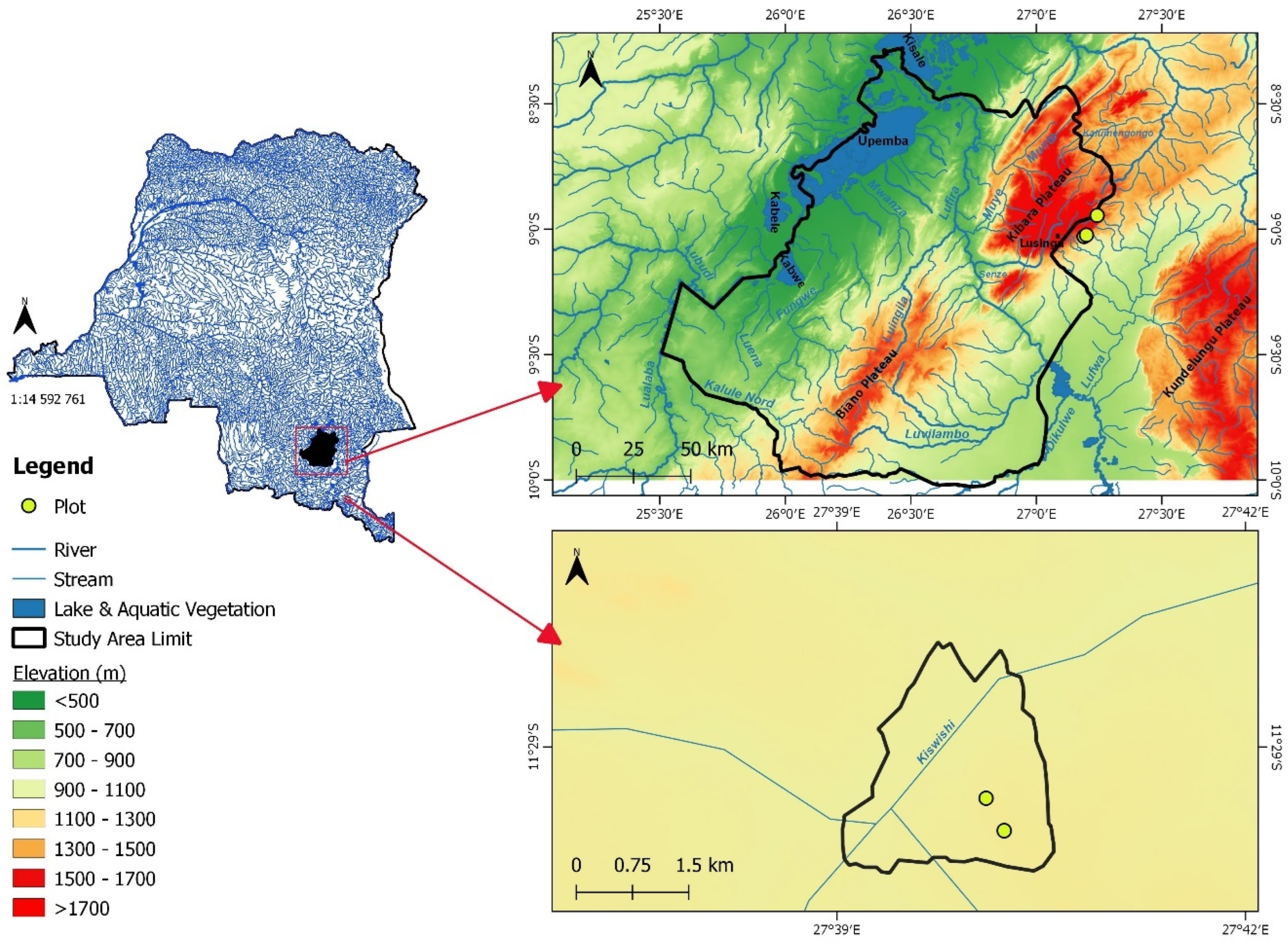
2.1. Study Sites and Data Collection

2.1.1. Study Sites

Data were collected in Mikembo Wildlife Reserve and Upemba National Park (UNP), both located in the Katanga region of DRC (Figure 1). These sites are characterised by a tropical climate with two distinct seasons of equal length [33,34].

UNP was created in 1939 in the heart of the Katanga province on an area of nearly 1,200,000 hectares. The initiative to create this protected area lies in the protection and conservation of a subspecies of zebra (Equus burchelii bohomi) endemic to the region [36]. Located in the Kamalondo depression, UNP hosts a matrix of grasslands, open forests, and gallery forests. In particular, the site is characterized by the presence of hills and high plateaus covered by open forests, where species of Monotes (Dipterocarpaceae) and Uapaca (Phillanthaceae) genus dominate. Approximately 10 km south of these plateaus, a plain shelters Miombo vegetation, characterized by a variety of species of Brachystegia and Isoberlinia (Detarioideae) genus. The soil on the plain is relatively deep and the litter layer thicker than in the open Monotes-Uapaca forests found on the plateaus and hills. During dry months, temperatures in the park range from 20 to 22 °C in the daytime and drop to 8 °C by night and average annual rainfall varies between 1200 to 1500 mm.

Mikembo reserve, located 1200 m a.s.l (at ca. 30–40 km northeast of Lubumbashi city), is an 800-ha private protected area where 442-ha of natural vegetation have been protected for at least fifteen years. The mean annual temperature and rainfall is 20.3 °C and 1240 mm, respectively. The dominant vegetation is typical wet Miombo woodland (characterized by species of genus Brachystegia spp., Julbernardia spp. and Marquesia macroura) with a sparse herbaceous stratum generally affected by high drainage during rainy season. This landscape has a flat topography with termite mounds up to 8 m high and the geological substrate of this area is characterized by dolomitic shales and siltstones from the Neoproterozoic, Nguba and Roan group [37]. For more details, we recommend reading also [38].

2.1.2. Data Collection

Forest Inventory Data

We set up two and three square 1 ha forest sample plots in Mikembo and UNP, respectively. Within each site, the choice of plots location was based on expert knowledge and aimed at sampling contrasted forest stands in terms of species composition and structure. Plot census protocol followed classical scientific forest inventory practices [39] and the Seosaw protocol [40]. Within each plot, the diameter at breast height (DBH) and taxonomic identification of all trees with DBH ≥ 10 cm were recorded. During the process of the establishment, plots were subdivided into 20 × 20 m quadrats and the relative coordinates of each censused tree within quadrats were recorded using a measuring tape and Suunto compass.

Terrestrial Laser Scanning Data

After plots census, each plot was scanned using a Leica C10 (https://cpec.leica-geosystems.com/fr/producto/leica-scanstation-c10/, accessed on 28 June 2025) terrestrial laser scanner following a systematic sampling design with one scan performed on each node of a regular grid of 20 m resolution (i.e., one scan on each quadrat corner). This resulted in a total of 36 scans per plot. The scanning resolution was set to “high”, corresponding to a point spacing of 5 cm at 100 m. The scanning protocol is described in detail in [27] and requires only two targets between scans (aka “backsight procedure”, [41]) to perform scans co-registration.

Wood Density Data

In addition to inventory and LiDAR data, we collected wood samples from a subset of trees within plots. For selected trees, wood samples were extracted from bark and pith slightly below the DBH measurement point, using a wood auger. After extraction, samples were directly stored in individual plastic straws and their fresh volume was recorded the same day using the volume displacement method [42,43,44]. After each field campaign, wood samples were brought to the laboratory. Dry mass was measured with a Kern and Sohn electronic scale with a capacity of 500 g and an accuracy of 0.001 g of all the samples after drying to constant weight (generally obtained after 60 to 72 h, depending on the tree species). Thus, the species Wood Density (WD) was computed as the ratio of dry weight over fresh volume. In total, we sampled 36 trees in Mikembo and 158 trees in UNP. Beside these data, we collected 425 additional WD estimates from Miombo forests species nearby Lubumbashi that were measured in the frame of previous projects [45]. Therefore, the total set of local WD estimates spans of 619 trees spread to over 81 species.

2.2. Methods

2.2.1. Terrestrial Laser Scanning Data Processing

For each forest sample plot, all TLS scans were co-registered using the automatic co-registration procedure implemented in Leica proprietary Cyclone software (v.9.2) based on forward and backward targets and point-based optimization. The full point cloud was then exported and underwent three main processing steps: (i) extraction of individual trees from the stand, (ii) for each tree, segmentation to separate leaf from wood points and (iii) from the cloud of wood points, reconstruction of the tree using quantitative structure modelling. The three processing steps mix automatic approaches using different algorithms and software (to obtain an initial result) and manual refinement of those initial results. The entire processing chain is described in [27] to which we refer the reader for details, and only provide a brief summary of each step hereafter:

-

An R code developed by Martin-ducup [27] was modified and used to automatically extract individual trees. For each tree, the code builds a cylindrical bounding box centered on that tree (using tree relative coordinates from forest inventory data) and sized so as to englobe the entire tree (using tree DBH from forest inventory data as well as height and crown diameter allometry models, [46]. The bounding box was then used to subset the stand points cloud and export points within the bounding box as a separate CSV file. The file was then imported into the 3Dforest software (Version 052) [16] for automatic ground removal, and into the CloudCompare software (Version V2.12) (Figure 2(C1–C3)) for a careful supervised refinement of the result i.e., the manual removal of points that do not belong to the focal tree.

-

An automatic wood/leaf segmentation was then performed on each focal tree using the algorithm developed by [17] in MATLAB iDSM (R2018a version). Subsequently, a manual correction of misclassified points (i.e., wood classified as leaf or vis versa) was performed in CloudCompare (Figure 2D).

-

Last, the TreeQSM algorithm (V.2.3.3, [15] was used on the focal tree wood points cloud to generate a quantitative structure model (QSM). The automatic QSM was then manually refined in AMAPStudio-Scan (Figure 2(E1,E2)), see also [22].

In this study, we extracted and processed 106 trees at the Mikembo site and 107 trees at the UNP site following the same guidelines for tree selection as for the collection of wood samples (i.e., preferentially targeting trees from abundant species and that spanned the entire DBH gradient found within plots). Following the processing of those trees, we measured their respective height (H) from the points cloud in 3Dforest.

Figure 2. TLS processing workflow. (A) One hectare Canopy Height Model (CHM) derived from scans co-registration. (B1,B2) Top and side views of target tree inside the cylindrical points cloud. (C1–C3) Different steps for tree extraction. (D) Leaf and wood segmentation. (E1,E2) Automated and manual editing QSMs.

Figure 2. TLS processing workflow. (A) One hectare Canopy Height Model (CHM) derived from scans co-registration. (B1,B2) Top and side views of target tree inside the cylindrical points cloud. (C1–C3) Different steps for tree extraction. (D) Leaf and wood segmentation. (E1,E2) Automated and manual editing QSMs.

2.2.2. Computation of Reference Aboveground Biomass Estimates

For each tree, the tree QSM was used to derive total tree volume by summing the volume of all QSM cylinders. Reference tree aboveground biomass estimates (AGB_TLS) were then computed by multiplying tree total volume by (i) the individual WD estimate when the tree was sampled in the field or (ii) the species average WD estimate from our local WD database when the tree was not sampled in the field. It is noteworthy that some tree species show marked within-tree variation of WD, notably along a vertical gradient (from the stump to the branch tips). Basal WD estimates—such as the ones we used—may therefore not be representative of the whole tree WD, thereby propagating errors on biomass estimates from TLS data. This issue has been studied on dense forests by [47] whom proposed a model based on basal WD and tree diameter to predict whole tree WD estimates. This model builds upon species ontogenetic and functional strategies which may differ between dense/wet forests and drier Miombo forests (see for instance [48,49]. For this reason, the correction model proposed in [47] was not implemented for the results presented in the main text of this study, but alternative sets of results that integrate this correction on WD—and hence AGB_TLS—can be found in Supplementary Materials.

2.2.3. Statistical Analyses

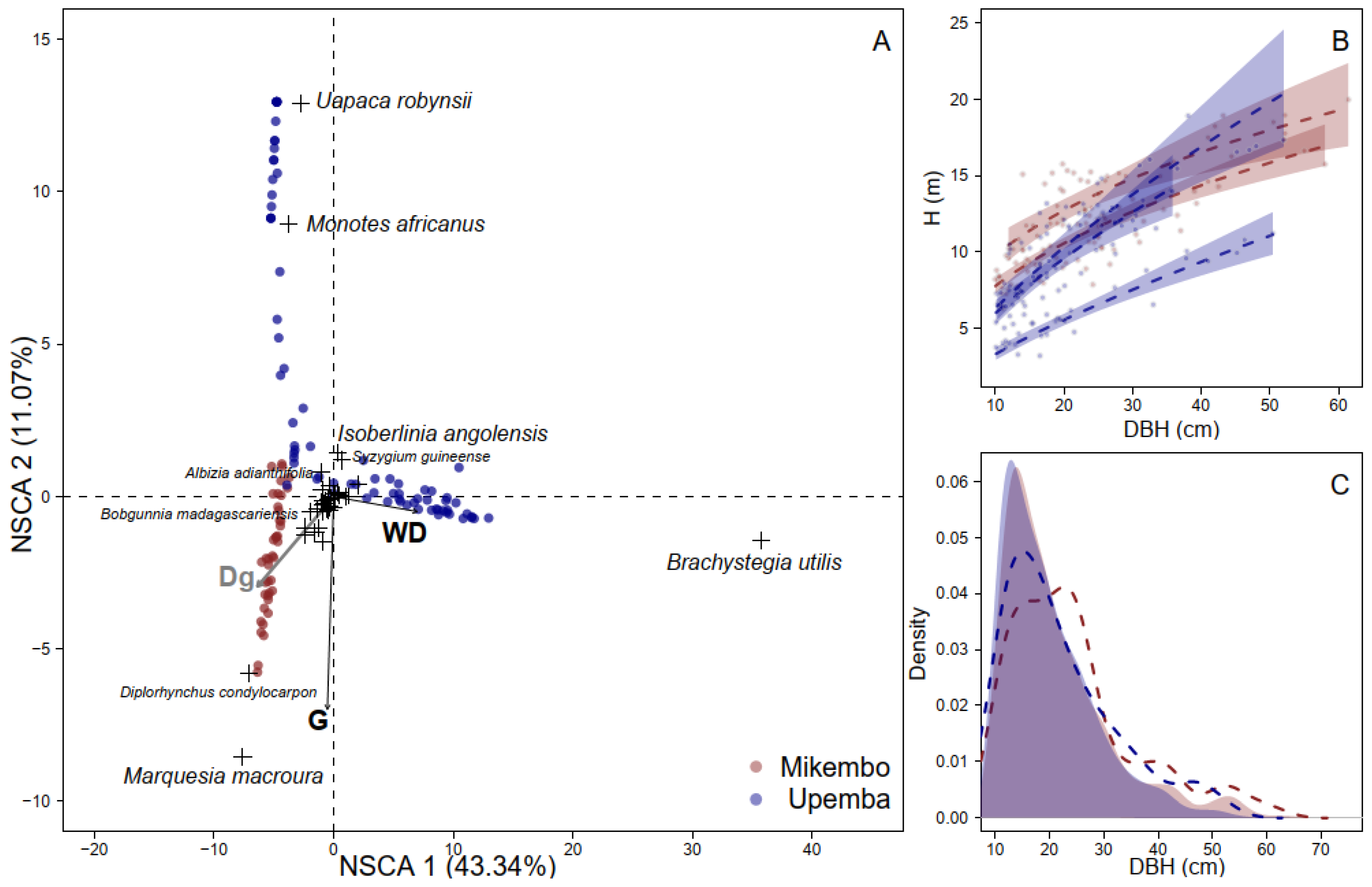
Flora Analysis

First, we analyze the flora composition from UNP and Mikembo in terms of species abundance, richness and frequency. We hypothesize that plots were distributed among a contrasted floristic assemblage. To illustrate this heterogeneity, we have used ade4 and vegan (Version 2.7-1 for vegan and Vesion 1.7-18 for ade4) packages to perform a Non-Symmetric Correspondence Analysis (NSCA) on the contingency table [50,51] of floristic data to obtain a synthetic description of the floristic variation. To fully capture the variation in the sampled stands, we introduce three additional variables: wood density (WD, g cm⁻³), mean diameter (Dg) and mean basal area (G, m² h⁻¹).

AGB Model Calibration

First, we selected a subset of 213 tree species as described in Section 2.2.1. For the sake of precision, we set up six DBH classes of 10 cm width, on which we performed the Chi² test of adequacy of distributions (with K⁻¹ degree of freedom) to check whether the subset had the same distribution as the original data. The results show that there is no significant difference in the distribution of trees in diameter classes between the two datasets (X-squared = 0.09762, df = 5, p-value = 0.9998 ns) assuming that the subset is representative of the original dataset.

We built four linear AGB allometric models on log-transformed data that are specified as follows:

$$\left(m1\right): log\left({AGB}_{TLS}\right)~ a + b \times log\left(DBH\right)+ \epsilon$$

(1)

$$\left(m2\right): log\left({AGB}_{TLS}\right) ~ a+b\times log\left(DB{H}^2\times H\right)+\epsilon$$

(2)

$$\left(m3\right): log\left({AGB}_{TLS}\right) ~ a+b\times log\left(DB{H}^2\times H\times W{D}_i\right)+\epsilon$$

(3)

$$\left(m4\right): log\left({AGB}_{TLS}\right) ~ a+b\times log\left(DBH\right)+c\times log\left(H\right)+d\times log\left({WD}_i\right)+\epsilon$$

(4)

with ${AGB}_{TLS}$ (in Kg) the reference tree aboveground biomass, DBH (in cm) the diameter at breast height, H (in m) the total tree height, $W{D}_i$ (in g cm⁻³) the tree wood density and ε the error term, which is assumed to follow a normal distribution N~(0, RSE²), where RSE is the Residual Standard Error of the model.

The model (m1) exclusively takes DBH as a predictor of AGB because it usually explains about half of AGB variation in tropical forests [52]. In addition to DBH, the second model (m2) integrates tree height and should thus provide a better approximation of tree volume [26,49,51]. Even more so that H-DBH relationships are known to be spatially structured [53,54] and thus to vary systematically between forest plots and sites [53]. This can result in stand level bias if the two variables are not accounted for. The third model (m3) combines DBH, H and $W{D}_i$ in a compound variable as in the widely-used pantropical AGB model [55], and should thus account for variation in WD among trees of similar volume. The last model (m4) includes three predictors of m3 but in separate terms and should provide a better fit than m3 at the cost of model generality. We assessed model fit using classical statistics: the coefficient of determination (R²), the Residual Standard Error (RSE), the Akaike Information Criterium (AIC) and Bayesian Information Criteria (BIC). We also quantified model uncertainty on back-transform predictions ($AG{B}_{pred}$) using the relative individual mean error (S, in %, Equation (5)) and the mean relative bias (B, in %, Equation (6)):

$$S={\displaystyle \frac{1}{n}}\times {\sum }_{i=1}^n\left({\displaystyle \frac{\left(AG{B}_{pred,i}-AG{B}_{TLS,i}\right)}{AG{B}_{TLS,i}}}\right)\times 100$$

(5)

$$B=\left({\displaystyle \frac{(\widehat{AG{B}_{pred}}-\widehat{AG{B}_{TLS}}}{\widehat{AG{B}_{TLS}}}}\right)\times 100$$

(6)

with i denoting individual trees. Due to the bias induced when back-transforming predictions from logarithmic to natural units (Kg), back-transformed AGB predictions were corrected using the Correction Factor (CF), $CF=e^{{\displaystyle \frac{RS{E}^2}{2}}}$ [55].

Model Cross-Validation

To assess model predictive performance, we first performed a 10-fold cross-validation (CV). This CV procedure consists of randomly splitting the tree dataset in 10 groups of equal size, then iteratively using nine folds for model calibration and the remaining fold for model testing. To further test models’ predictive performance outside sampled areas, we also used a leave-one-site-out model CV, which consisted in training models on data from one site and predicting tree AGB on data from the left-out site. For each CV procedure, we used back-transformed AGB predictions to compute a pseudo-R² (i.e., the squared correlation between $AG{B}_{pred}$ and $AG{B}_{TLS}$) as well as the S and B statistics described above (Equations (5) and (6)).

Comparison of Local and Literature-Based Model Predictions

Tree AGB predictions derived from the best local model were compared to those of AGB models from the literature, notably (i) the pantropical model of Chave et al. [55], (ii) the regional model of Fayolle et al. [56] as well as (iii) models built on trees of Miombo forests, namely by Chidumayo [57] and Mugasha et al. [58,59] which were applied in Zambia and Tanzania, respectively. Comparison with existing models is a good way of validating and better understanding the variation of AGB across the region by using different models [60].

All data analyses were performed on the R (Version 2.1.8. for BIOMASS; Version 2.5 pour Factoshiny; Agricolae 1.3.5) statistical platform [61] using mainly the following packages: BIOMASS [62], Factoshiny [63], Agricolae [64] and Vegan [65].

3. Results

3.1. Floristic Structure

Among the 1667 trees censused on the five forest plots, we identified 61 species, 39 genera and 20 families (while 2 trees remained unidentified). The five most represented families on both sites are Fabaceae (57.47%), Dipterocarpaceae (14.70%), Apocynaceae (8.98%), Phyllanthaceae (8.34%) and Myrtaceae (2.88%). In terms of genera, Brachystegia (34.49%), Monotes (7.50%), Marquesia (7.20%), Diplorhynchus (7.08%) and Uapaca (7.02%) are the five most represented groups. Approximately half of the species (n = 30) were encountered at both sampling sites.

The first two NSCA axes explained 54.41% of the total variance in the data. The first axis opposed quadrats characterized by the abundance of Brachystegia utilis (from two 1-ha plots at the Upemba site, Figure 3A) compared to the other quadrats. The second axis opposed quadrats from the third Upemba plot on its positive side, which was dominated by the species Uapaca robynsii and Monotes africanus—compared to quadrats from the Mikembo site, which were on its negative side and were characterized by the abundance of the species Marquesia macroura and Diplorhynchus condylocarpon.

Floristic assemblages influenced the average wood density found at quadrat level (WD), which positively correlated with the first NSCA axis (Figure 3A) and indicated a higher average wood density for Upemba‘s quadrats dominated by Brachystegia utilis—which had a relatively high species-level wood density (c. 0.83 g·cm⁻³). From the structural standpoint, Mikembo’s plots had a larger basal area on average (i.e., 22.75 m²·ha⁻¹) than UNP’s plots (11.18 m²·ha⁻¹) due to the presence of larger trees (Figure 3C), notably at Mik2 (G: 30.1 m²·ha⁻¹). This between-site difference was reflected in the size-distribution of trees selected for allometry model building (Figure 3C, dashed lines). Lastly, canopy height and H: DBH allometry were homogeneous across plots at the exception of UP3, where trees reached much lower heights for similar DBHs (Figure 3B).

3.2. Calibrating and Validating Allometry Models

Using the set of 213 scanned trees to calibrate AGB allometry models, we found that each model’s functional form performed relatively well (R² > 0.9,

Table 1. Statistics of AGB models calibration fit. Models’ predictors include the diameter at breast height (DBH in cm), the mean specific wood density (WDi in g·cm⁻³), the total tree height (H in m), and tree aboveground biomass (AGB), in kg. Provided statistics include the share variance explained (R²), the residual standard error (RSE), the AIC, the BIC, the relative individual mean error (S, in %) and the mean relative bias (B, in M·g). Model coefficient estimates (a, b, c and d) are provided along with standard error (SE).

Model	Performance Criteria						Coefficient Estimates (±SE)
	R2	RSE	AIC	BIC	S	B	a	b	c	d
(m1) log (AGB) ~ a + b × log (DBH)	0.91	0.37	193.90	203.99	16.34	2.78	−2.6230 (±0.1792)	2.6338 (±0.0584)	-	-
(m2) log (AGB) ~ a + b × log (DBH2 × H)	0.90	0.38	198.19	208.28	15.67	−0.27	−2.9297 (±0.1881)	0.9920 (±0.0222)	-	-
(m3) log (AGB) ~ a + b × log (DBH2 × H × WDi)	0.92	0.34	154.62	164.70	12.65	−0.71	−2.4368 (±0.1585)	0.9790 (±0.0196)	-	-
(m4) log (AGB) ~ a + b × log (DBH) + c × log (H) + d × log (WDi)	0.93	0.32	137.15	153.96	11.73	0.53	−2.2499 (±0.1974)	1.0871 (±0.0378)	0.6485 (±0.0853)	1.2101 (±0.2124)

). As expected, the successive addition of key additional AGB predictors (from m1 to m3) gradually improved model fit by increasing the share of variance explained (R²) and decreasing tree-level mean percent error (S) and model’s AIC (Table 1). Further, splitting the compound predictor variable of m3 into three separate predictors in m4 led to an additional improvement in fit statistics (AIC of 154.63 vs. 137.15 for m3 and m4, respectively).

To assess the generality of AGB models, we performed a random 10-fold and a leave-one-site-out model CVs. CV statistics show that models m1 and m4 tend to explain slightly more variation in tree AGB than m2 and m3, but with relatively similar or higher levels of tree- and plot-level biases (

Table 2. Statistics of AGB models predictive performance from random and leave-one-site-out model CV. Models’ predictors include the diameter at breast height (DBH in cm), the mean specific wood density ($\mathrm{W}{\mathrm{D}}_{\mathrm{i}}$ in g cm⁻³) and the total tree height (H in m), and the tree aboveground biomass (AGB) in kg. Provided statistics include the share variance explained (R²), the relative individual mean error (S, in %) and the mean relative bias (B, in M·g).

Models	10-Fold CV			Spatial CV
	R2	S	B	R2	S	B
(m1) AGB_kg = 0.0718 × DBH2.6338	0.91	16.41	2.92	0.91	19.45	3.52
(m2) AGB_kg = 0.0534 × (DBH2 × H)0.992	0.87	15.75	−0.21	0.87	16.11	2
(m3) AGB_kg = 0.0927 × (D2 × H × WDi)0.979	0.90	12.72	−0.64	0.90	12.86	0.22
(m4) AGB_kg = 0.1054× DBH1.0871 × H0.6485 × WDi1.210	0.91	14.70	3.22	0.90	17.13	3.68

). In the case of the 10-fold random CV for example, R² values for m1 and m4 was 0.91 against 0.88 for m2 and 0.90 for m3, but their plot-level bias (B) was close to 3 M·g. against B < 1 M·g. for both m2 and m3. This pattern is explained by the better predictive performance of m2 and m3 on small and medium sized trees—which dominates the dataset and disproportionally affect bias metrics—while m1 and m4 slightly outperform m2 and m3 on the few large trees. Further, the leave-one-site-out CV confirmed the higher generality of m3’s functional form which better transposed to new sites, with lower tree- and plot-level prediction biases than any other models (i.e., S = 12.86% and B = 0.22 M·g, Table 2).

3.3. Comparing Local Allometry Equations with State of Art

Aboveground biomass predictions derived from the m3 AGB model were compared with predictions from the pantropical model (denoted as Chave et al. (2014) [55] in Figure 4), a regional model (denoted as Fayolle et al. 2018) [42] as well as two local models developed on Miombo’s forests in neighboring countries (denoted as Chidumayo (2013) [57] and Mugasha et al. (2013)) [59]. Overall, this comparison shows that AGB models from literature tend to underestimate tree AGB in the wet Miombo forests of DRC, which is particularly evident for trees larger than 1000 kg (Figure 4A), while predictions from the model m3 developed in this study are closer to a 1:1 line. Across all trees, the underestimation observed by AGB models from the literature lead to a substantial negative bias of c. 29.58–35.04% for the pantropical and regional model, and of c. 19.97–21.47% for models developed on Miombo forests (Figure 4B).

4. Discussion

4.1. Floristic Communities

The survey carried out on the two sites showed that the flora is mainly dominated by Detarioideae species. The predominance of this family reveals that the two sites are mainly home to miombo type vegetation [32,67]. The projection of the flora in an NSCA analysis showed the distinction of three distinct plant communities. The community with Brachystegia and Isoberlinia is classified as being in the Mesobrachytegion phytosociological alliance. The latter is a type of vegetation growing on generally deep colluvial soils on the hillside [68]. The second is that of the Marquesia and the Julbernardia, which he classifies as being in the Berlinio-Marquesion, a type of vegetation found on flat ground, and which are relics of dense dry forests. While a third community is that of Uapaca and Monotes which the same author classifies in the Xerobrachystegion. It is a type of vegetation developing on rocky, xeric substrates, with a superficial horizon very poor in clay and organic matter than the previous ones [68,69]. These types of vegetation have also been encountered elsewhere, such as in Zambia [57], Tanzania [70]. These results show that the vegetation used to establish this allometry equation is both varied and representative of forest ecosystems evolving in the landscape of the Miombo ecoregion in Haut-Katanga. Additionally, the high abundance of D. condylocarpon which is an heliophilous undergrowth species [71], tolerant to bush fire [72] confirms that the Mikembo forest is more degraded than the Upemba forest and can therefore be considered as representative of a forest that is recovering after a degradation process.

4.2. Allometric Models

We calibrated a set of allometry models using a relatively large dataset (213 trees, i.e., more than all previous studies in the region [55,56,57,58,59,73] and covering a representative DBH (10 to 61.4 cm) and wood density range.

The protocol used for terrestrial LiDAR scanning data acquisition and processing follows currently established standards with the addition of careful manual check. This last step can make substantial difference as previously shown [22,27]. During calibration of allometry equations (AEs), DBH measured from our floristic survey were used instead of those derived from TLS to avoid possible cross-modality error in DBH estimation [22,74], as the developed models are targeted to an operational use within traditional forest inventories, and in particular the DRC National Forest Inventory. Also, Tree height (H) was derived from the TLS point clouds by identifying the highest point associated with each segmented tree. TLS generally improves accuracy compared to manual or LiDAR aerial approaches; some uncertainty remains due to factors such as occlusion, scan angle or canopy density, and crown complexity. Recent studies in tropical forests have quantified the accuracy of TLS-derived height estimates, reporting root mean square errors (RMSEs) typically ranging between 0.5 and 1.5 m, depending on forest structure and scanning configuration [25]. During our field work, all scans were performed in high resolution which means that 0.05 m between points at 100 m [22].

Cross-validation showed the AE models calibrated in this study—and particularly the m3 model—were transposable across sites within wet Miombo, despite strong difference in forest composition and structure. Surprisingly, the simplest model accounting only for DBH worked nearly as well as model m4 which also accounted for tree height and wood density. It is worth noting however that the cross-validation was performed at the site level, whereas H-DBH (and WD) have been shown (including in this study) to present their largest variability locally between plots rather than across sites. This is notably because H-DBH relationships are largely modulated by the competition for light (e.g., through stand basal area) [54]. The Miombo being open, this modulation might arguably be less intense than in denser forested ecosystems, but this would deserve more in-depth study before concluding that local H-DBH relationship can be disregarded for the estimation of AGB in Miombo forest. Regarding wood density, it is of course impacted by the local history of perturbation and succession, but it has been shown to be a less important descriptor even in dense forest ecosystems, in terms of explained inter-site variance in AGB [75,76]

4.3. Comparison with Models from State of Art

Published allometry models seem to underestimate AGB from our Miombo trees with an overall bias ranging from c. −35% to c. −20%. This underestimation is more important for equations calibrated in other forest types [54] different from the Miombo [57,59]. In particular, despite its remarkable calibration dataset (845 tropical trees, 55 species covering a wide range in diameter up to 200 cm), the regional model of [42] yielded the largest bias, which we attribute to the fact that all six forest strata sampled in this study were not structurally and floristically close to Miombo. This contrast with the pantropical AGB model [55]—which included data from two Miombo forest sites in its calibration set and yielded the second largest bias. However, these data only represented 142 trees over a total sample of more than 4000 trees. Our results are in line with previous studies showing that large systematic deviations in model predictions may occur when AGB models are applied on forest strata that differ from that on which they were calibrate. For example, [42] reported a bias of nearly 80% in AGB when applying a model developed on a tropical moist forest to a wet Miombo forest. Such biases have also been explored in other studies [56]. Finally, allometry equations adjusted in Miombo from neighboring countries produced a more moderate—but still noteworthy—bias. The AE from [57] yielded the closest AGB predictions to our reference trees. Interestingly, the tree dataset used in the latter study shares the same dominant flora composition (Brachystegia boehmii, B. manga, B. spiciformis, Julbernardia globiflora, Isoberlinia angolensis and Uapaca spp.) as [59]. The Chidumayo model yields the closest predictions to ours, as the site is also in the Wet Miombo type and shares the same dominant Flora. The Mugasha model presents larger differences, being calibrated in dry Miombo forest. These results show that injecting miombo species into the model tends to bring biomass estimators closer together. Finally, we noticed that the Fayolle’s model, which does not include any miombo species, induces a greater bias than the others. As we move closer to our study area, the bias decreases. Bias can therefore vary geographically, but also according to the biome or vegetation type considered in the development of regional pantropical models. These findings highlight the importance of locally calibrated models for accurate biomass estimation in Miombo ecosystems.

5. Conclusions

This study fills an important gap by developing specific allometric equations for estimating aboveground biomass (AGB) in the Miombo forests of the Democratic Republic of Congo (DRC). To minimize errors in the results obtained, we used a combination of methodological tools to evaluate AGB and allometry equations in a non-destructive and robust way. Our analysis demonstrates that TLS measurements can be efficiently converted into AGB (with quantitative structure models and wood density) and help to rapidly construct an allometry equation for Miombo.

We found that the use of regional or pantropical allometry equations produces a significant bias in the prediction of Miombo biomass in Upper Katanga that we attribute to the limited representativeness of this forest type in global tree biomass databases. This may also be true for the other forest biomes of the Miombo ecoregion. It would therefore be necessary to produce specific equations for each biome to avoid large systematic error in biomass predictions, which would be detrimental to the scaling up necessary for monitoring ecosystem dynamics within the MRV framework—Monitoring, Reporting and Verification—to support the REDD+ process and achieve sustainable development goals.

References

1. Goodman, R.; Herold, M. Why Maintaining Tropical Forests is Essential and Urgent for a Stable Climate; Center for Global Development Working Paper, no 385; Center for Global Development: Washington, DC, USA, 2014. [Google Scholar] [CrossRef]
2. Chave, J.; Davies, S.J.; Phillips, O.L.; Lewis, S.L.; Sist, P.; Schepaschenko, D.; Armston, J.; Baker, T.R.; Coomes, D.; Disney, M.; et al. Ground Data are Essential for Biomass Remote Sensing Missions. Surv. Geophys. 2019, 40, 863–880. [Google Scholar] [CrossRef]
3. Calders, K.; Verbeeck, H.; Burt, A.; Origo, N.; Nightingale, J.; Malhi, Y.; Wilkes, P.; Raumonen, P.; Bunce, R.G.H.; Disney, M. Laser scanning reveals potential underestimation of biomass carbon in temperate forest. Ecol. Solut. Evid. 2022, 3, e12197. [Google Scholar] [CrossRef]
4. IPCC SESSION OF THE IPCC 8–12 May 2019, Kyoto, Japan Decisions adopted by the Panel Decision IPCC-XLIX-1. Adoption of the Provisional Agenda. 2019, 1–17. Available online: https://www.ipcc.ch/site/assets/uploads/2019/05/IPCC-49_decisions_adopted.pdf (accessed on 28 June 2025).
5. Calders, K.; Newnham, G.; Burt, A.; Murphy, S.; Raumonen, P.; Herold, M.; Culvenor, D.; Avitabile, V.; Disney, M.; Armston, J.; et al. Nondestructive estimates of above-ground biomass using terrestrial laser scanning. Methods Ecol. Evol. 2015, 6, 198–208. [Google Scholar] [CrossRef]
6. Dassot, M.; Constant, T.; Fournier, M. The use of terrestrial LiDAR technology in forest science: Application fields, benefits and challenges. Ann. For. Sci. 2011, 68, 959–974. [Google Scholar] [CrossRef]
7. Dassot, M.; Colin, A.; Santenoise, P.; Fournier, M.; Constant, T. Terrestrial laser scanning for measuring the solid wood volume, including branches, of adult standing trees in the forest environment. Comput. Electron. Agric. 2012, 89, 86–93. [Google Scholar] [CrossRef]
8. Demol, M.; Verbeeck, H.; Gielen, B.; Armston, J.; Burt, A.; Disney, M.; Duncanson, L.; Hackenberg, J.; Kükenbrink, D.; Lau, A.; et al. Estimating forest above-ground biomass with terrestrial laser scanning: Current status and future directions. Methods Ecol. Evol. 2022, 13, 1628–1639. [Google Scholar] [CrossRef]
9. Demol, M.; Calders, K.; Verbeeck, H.; Gielen, B. Forest above-ground volume assessments with terrestrial laser scanning: A ground-truth validation experiment in temperate, managed forests. Ann. Bot. 2021, 128, 805–819. [Google Scholar] [CrossRef]
10. Disney, M.; Burt, A.; Wilkes, P.; Armston, J.; Duncanson, L. New 3D measurements of large redwood trees for biomass and structure. Sci. Rep. 2020, 10, 16721. [Google Scholar] [CrossRef]
11. Malhi, Y.; Jackson, T.; Patrick Bentley, L.; Lau, A.; Shenkin, A.; Herold, M.; Calders, K.; Bartholomeus, H.; Disney, M.I. New perspectives on the ecology of tree structure and tree communities through terrestrial laser scanning. Interface Focus. 2018, 8, 20170052. [Google Scholar] [CrossRef]
12. Åkerblom, M.; Kaitaniemi, P. Terrestrial laser scanning: A new standard of forest measuring and modelling? Ann. Bot. 2021, 128, 653–662. [Google Scholar] [CrossRef] [PubMed]
13. Markku, Å.; Raumonen, P.; Kaasalainen, M.; Casella, E.; Markku, Å.; Raumonen, P.; Kaasalainen, M.; Casella, E. Analysis of Geometric Primitives in Quantitative Structure Models of Tree Stems. Remote Sens. 2015, 7, 4581–4603. [Google Scholar] [CrossRef]
14. Hackenberg, J.; Spiecker, H.; Calders, K.; Disney, M.; Raumonen, P. SimpleTree—An efficient open-source tool to build tree models from TLS clouds. Forests 2015, 6, 4245–4294. [Google Scholar] [CrossRef]
15. Raumonen, P.; Kaasalainen, M.; Akerblom, M.; Kaasalainen, S.; Kaartinen, H.; Vastaranta, M.; Holopainen, M.; Disney, M.; Lewis, P. Fast automatic precision tree models from terrestrial laser scanner data. Remote Sens. 2013, 5, 491–520. [Google Scholar] [CrossRef]
16. Trochta, J.; Kruček, M.; Vrška, T.; Kraâl, K. 3D Forest: An application for descriptions of three-dimensional forest structures using terrestrial LiDAR. PLoS ONE 2017, 12, e0176871. [Google Scholar] [CrossRef] [PubMed]
17. Wang, D.; Momo Takoudjou, S.; Casella, E. LeWoS: A universal leaf-wood classification method to facilitate the 3D modelling of large tropical trees using terrestrial LiDAR. Methods Ecol. Evol. 2020, 11, 376–389. [Google Scholar] [CrossRef]
18. Wilkes, P.; Disney, M.; Armston, J.; Bentley, L.; Brede, B.; Burt, A.; Calders, K.; Chavana-Bryant, C.; Clewley, D.; Duncanson, L.; et al. TLS2trees: A scalable tree segmentation pipeline for TLS data. bioRxiv 2022, 24. [Google Scholar] [CrossRef]
19. Bogdanovich, E.; Perez-Priego, O.; El-Madany, T.S.; Guderle, M.; Pacheco-Labrador, J.; Levick, S.R.; Moreno, G.; Carrara, A.; Martín, M.P.; Migliavacca, M. Using terrestrial laser scanning for characterizing tree structural parameters and their changes under different management in a Mediterranean open woodland. For. Ecol. Manag. 2021, 486, 118945. [Google Scholar] [CrossRef]
20. Burt, A.; Disney, M.; Calders, K. Extracting individual trees from lidar point clouds using treeseg. Methods Ecol. Evol. 2019, 10, 438–445. [Google Scholar] [CrossRef]
21. Hackenberg, J.; Wassenberg, M.; Spiecker, H.; Sun, D. Non-Destructive Method for Biomass Prediction Combining TLS Derived Tree Volume and Wood Density. Forests 2015, 6, 1274–1300. [Google Scholar] [CrossRef]
22. Momo Takoudjou, S.; Ploton, P.; Sonké, B.; Hackenberg, J.; Griffon, S.; De Coligny, F.; Kamdem, N.G.; Libalah, M.; Mofack, G.I.; Le Moguédec, G.; et al. Using terrestrial laser scanning data to estimate large tropical trees biomass and calibrate allometric models: A comparison with traditional destructive approach. Methods Ecol. Evol. 2018, 9, 905–916. [Google Scholar] [CrossRef]
23. Raumonen, P.; Casella, E.; Calders, K.; Murphy, S.; Åkerblom, M.; Kaasalainen, M. Massive-scale tree modelling from TLS data. ISPRS Ann. Photogramm. Remote Sens. Spat. Inf. Sci. 2015, 2, 189–196. [Google Scholar] [CrossRef]
24. Woodgate, W.; Jones, S.D.; Suarez, L.; Hill, M.J.; Armston, J.D.; Wilkes, P.; Soto-Berelov, M.; Haywood, A.; Mellor, A. Understanding the variability in ground-based methods for retrieving canopy openness, gap fraction, and leaf area index in diverse forest systems. Agric. For. Meteorol. 2015, 205, 83–95. [Google Scholar] [CrossRef]
25. Abd Rahman, M.Z.; Abu Bakar, M.A.; Razak, K.A.; Rasib, A.W.; Kanniah, K.D.; Wan Kadir, W.H.; Omar, H.; Faidi, A.; Kassim, A.R.; Abd Latif, Z. Non-destructive, laser-based individual tree aboveground biomass estimation in a tropical rainforest. Forests 2017, 8, 86. [Google Scholar] [CrossRef]
26. Phalla Thuch Ota Tetsuji Mizoue Nobuya et, a.l. The importance of tree height in estimating individual tree biomass while considering errors in measurements and allometric models. AGRIVITA J. Agric. Sci. 2017, 40, 131–140. [Google Scholar]
27. Martin-Ducup, O.; Mofack, G.; Wang, D.; Raumonen, P.; Ploton, P.; Sonké, B.; Barbier, N.; Couteron, P.; Pélissier, R. Evaluation of automated pipelines for tree and plot metric estimation from TLS data in tropical forest areas. Ann. Bot. 2021, 128, 753–765. [Google Scholar] [CrossRef] [PubMed]
28. Trochta, J.; Král, K.; Janík, D.; Adam, D. Arrangement of terrestrial laser scanner positions for area-wide stem mapping of natural forests. Can. J. For. Res. 2013, 43, 355–363. [Google Scholar] [CrossRef]
29. Timberlake, J.; Chidumayo, E. Division report. IEEE Control Syst. Mag. 2004, 3, 25. [Google Scholar] [CrossRef]
30. Ribeiro, N.S.; Silva de Miranda, P.L.; Timberlake, J. Biogeography and ecology of miombo woodlands. In Miombo Woodlands in a Changing Environment: Securing the Resilience and Sustainability of People and Woodlands; Springer International Publishing: Cham, Switzerland, 2020; pp. 9–53. [Google Scholar]
31. Tarimo, B.; Dick, Ø.B.; Gobakken, T.; Totland, Ø. Spatial distribution of temporal dynamics in anthropogenic fires in miombo savanna woodlands of Tanzania. Carbon Balance Manag. 2015, 10, 18. [Google Scholar] [CrossRef]
32. Campbell, B. The Miombo in Transition: Woodlands and Welfare in Africa; CIFOR, Center for International Forestry Research (CIFOR): Bogor, Indonesia, 1996; 273p. [Google Scholar]
33. Ilunga Muledi, J.; Bauman, D.; Drouet, T.; Vleminckx, J.; Jacobs, A.; Lejoly, J.; Meerts, P.; Shutcha, M.N. Fine-scale habitats influence tree species assemblage in a miombo forest. J. Plant Ecol. 2016, 10, rtw104. [Google Scholar] [CrossRef]
34. Bauman, D.; Raspe, O.; Meerts, P.; Degreef, J.; Ilunga Muledi, J.; Drouet, T. Multiscale assemblage of an ectomycorrhizal fungal community: The influence of host functional traits and soil properties in a 10-ha miombo forest. FEMS Microbiol. Ecol. 2016, 92, 151. [Google Scholar] [CrossRef]
35. Chirwa, P.; Syampungani, S.; Geldenhuys, C.J. The ecology and management of the Miombo woodlands for sustainable livelihoods in southern Africa: The case for non-timber forest products. South. For. J. For. Sci. 2008, 70, 237–245. [Google Scholar] [CrossRef]
36. Des, E.; Unis, E.; Washington, S.N.W. Parcs et Réserves de la République Démocratique du Congo Parcs et réserves de la République Démocratique du Congo. 2015; 1–149. Available online: https://papaco.org/wp-content/uploads/2015/09/RAPPAM-RDC-impression-110629-A4.pdf (accessed on 28 June 2025).
37. Batumike, M.J.; Kampunzu, A.B.; Cailteux, J.H. Petrology and geochemistry of the Neoproterozoic Nguba and Kundelungu Groups, Katangan Supergroup, southeast Congo: Implications for provenance, paleoweathering and geotectonic setting. J. Afr. Earth Sci. 2006, 44, 97–115. [Google Scholar] [CrossRef]
38. KayaMuyumba D._2015. Available online: https://doaj.org/article/f6853ed0ff8a4912a100ec46f1aa2ce6 (accessed on 28 June 2025).
39. Phillips, O.; Baker, T.; Feldpausch, T.; Brienen, R. RAINFOR Field Manual for Plot Establishment and Remeasurement. 2009. Available online: https://forestplots.net/upload/manualsenglish/rainfor_field_manual_en.pdf (accessed on 28 June 2025).
40. SEOSAW partnership. A network to understand the changing socio-ecology of the southern African woodlands (SEOSAW): Challenges, benefits, and methods. Plants People Planet 2021, 3, 249–267. [Google Scholar] [CrossRef]
41. Wang, Z. Real-Time Updated free Station as a Georeferencing Method in Terrestrial Laser Scanning. 2011. Available online: http://www.diva-portal.org/smash/get/diva2:423230/FULLTEXT01.pdf (accessed on 28 June 2025).
42. Fayolle, A.; Ngomanda, A.; Mbasi, M.; Barbier, N.; Bocko, Y.; Boyemba, F.; Couteron, P.; Fonton, N.; Kamdem, N.; Katembo, J.; et al. A regional allometry for the Congo basin forests based on the largest ever destructive sampling. For. Ecol. Manag. 2018, 430, 228–240. [Google Scholar] [CrossRef]
43. Henry, M.; Besnard, A.; Asante, W.A.; Eshun, J.; Adu-Bredu, S.; Valentini, R.; Bernoux, M.; Saint-André, L. Wood density, phytomass variations within and among trees, and allometric equations in a tropical rainforest of Africa. For. Ecol. Manag. 2010, 260, 1375–1388. [Google Scholar] [CrossRef]
44. Vieilledent, G.; Vaudry, R.; Andriamanohisoa, S.F.; Rakotonarivo, O.S.; Randrianasolo, H.Z.; Razafindrabe, H.N.; Rakotoarivony, C.B.; Ebeling, J.; Rasamoelina, M. A universal approach to estimate biomass and carbon stock in tropical forests using generic allometric models. Ecol. Appl. 2012, 22, 572–583. [Google Scholar] [CrossRef]
45. Muledi, J.; Bauman, D.; Jacobs, A.; Meerts, P.; Shutcha, M.; Drouet, T. Tree growth, recruitment, and survival in a tropical dry woodland: The importance of soil and functional identity of the neighbourhood. For. Ecol. Manag. 2020, 460, 117894. [Google Scholar] [CrossRef]
46. Martinez Cano, I.; Muller-Landau, H.C.; Wright, S.J.; Bohlman, S.A.; Pacala, S.W. Interspecific variation in tropical tree height and crown allometries in relation to life history traits. Biogeosci. Discuss. 2018, 16, 847–862. [Google Scholar] [CrossRef]
47. Momo, S.T.; Ploton, P.; Martin-Ducup, O.; Lehnebach, R.; Fortunel, C.; Sagang, L.B.T.; Boyemba, F.; Couteron, P.; Fayolle, A.; Libalah, M.; et al. Leveraging Signatures of Plant Functional Strategies in Wood Density Profiles of African Trees to Correct Mass Estimations from Terrestrial Laser Data. Sci. Rep. 2020, 10, 2001. [Google Scholar] [CrossRef]
48. Lohbeck, M.; Lebrija-Trejos, E.; Martínez-Ramos, M.; Meave, J.A.; Poorter, L.; Bongers, F. Functional Trait Strategies of Trees in Dry and Wet Tropical Forests Are Similar but Differ in Their Consequences for Succession. PLoS ONE 2015, 10, e0123741. [Google Scholar] [CrossRef]
49. Poorter, L.; Rozendaal, D.M.A.; Bongers, F.; de Almeida-Cortez, J.S.; Almeyda Zambrano, A.M.; Álvarez, F.S.; Andrade, J.L.; Villa, L.F.A.; Balvanera, P.; Becknell, J.M.; et al. Wet and dry tropical forests show opposite successional pathways in wood density but converge over time. Nat. Ecol. Evol. 2019, 3, 928–934. [Google Scholar] [CrossRef]
50. Lombardo, R.; Beh, E.J.; Lombardo, M.R. Package ‘CAvariants’. Medicine 2017, 57, 947–961. [Google Scholar]
51. Lombardo, R.; Beh, E.J.; D’Ambra, L. Non-symmetric correspondence analysis with ordinal variables using orthogonal polynomials. Comput. Stat. Data Anal. 2007, 52, 566–577. [Google Scholar] [CrossRef]
52. Molto, Q.; Hérault, B.; Boreux, J.J.; Daullet, M.; Rousteau, A.; Rossi, V. Predicting tree heights for biomass estimates in tropical forests -A test from French Guiana. Biogeosciences 2014, 11, 315021–315030. [Google Scholar] [CrossRef]
53. Loubota Panzou, G.J.; Fayolle, A.; Jucker, T.; Phillips, O.L.; Bohlman, S.; Banin, L.F.; Lewis, S.L.; Affum-Baffoe, K.; Alves, L.F.; Antin, C.; et al. Pantropical variability in tree crown allometry. Glob. Ecol. Biogeogr. 2020, 30, 459–475. [Google Scholar] [CrossRef]
54. Feldpausch, T.R.; Banin, L.; Phillips, O.L.; Baker, T.R.; Lewis, S.L.; Quesada, C.A.; Affum-Baffoe, K.; Arets, E.J.M.M.; Berry, N.J.; Bird, M.; et al. Height-diameter allometry of tropical forest trees. Biogeosciences 2011, 8, 1081–1106. [Google Scholar] [CrossRef]
55. Chave, J.; Réjou-Méchain, M.; Búrquez, A.; Chidumayo, E.; Colgan, M.S.; Delitti, W.B.C.; Duque, A.; Eid, T.; Fearnside, P.M.; Goodman, R.C.; et al. Improved allometric models to estimate the aboveground biomass of tropical trees. Glob. Chang. Biol. 2014, 20, 3177–3190. [Google Scholar] [CrossRef]
56. Fayolle, A.; Doucet, J.L.; Gillet, J.F.; Bourland, N.; Lejeune, P. Tree allometry in Central Africa: Testing the validity of pantropical multi-species allometric equations for estimating biomass and carbon stocks. For. Ecol. Manag. 2013, 305, 29–37. [Google Scholar] [CrossRef]
57. Chidumayo, E.N. Estimating tree biomass and changes in root biomass following clear-cutting of Brachystegia-Julbernardia (miombo) woodland in central Zambia. Environ. Conserv. 2013, 41, 54–63. [Google Scholar] [CrossRef]
58. Mugasha, W.A.; Mwakalukwa, E.E.; Luoga, E.; Malimbwi, R.E.; Zahabu, E.; Silayo, D.S.; Sola, G.; Crete, P.; Henry, M.; Kashindye, A. Allometric models for estimating tree volume and aboveground biomass in lowland forests of Tanzania. Int. J. For. Res. 2016, 2016, 8076271. [Google Scholar] [CrossRef]
59. Mugasha, W.A.; Eid, T.; Bollandsås, O.M.; Malimbwi, R.E.; Chamshama, S.A.O.; Zahabu, E.; Katani, J.Z. Allometric models for prediction of above and belowground biomass of trees in the miombo woodlands of Tanzania. For. Ecol. Manag. 2013, 310, 87–101. [Google Scholar] [CrossRef]
60. Liu, B.; Bu, W.; Zang, R. Improved allometric models to estimate the aboveground biomass of younger secondary tropical forests. Glob. Ecol. Conserv. 2023, 41, e02359. [Google Scholar] [CrossRef]
61. R Core Team. R: A Language and Environment for Statistical Computing; R Foundation for Statistical Computing: Vienna, Austria, 2008; Available online: http://www.R-project.org/ (accessed on 10 June 2025).
62. Réjou-Méchain, M.; Tanguy, A.; Piponiot, C.; Chave, J.; Hérault, B. Biomass: An R Package for Estimating Above-Ground Biomass and Its Uncertainty in Tropical Forests. Methods Ecol. Evol. 2017, 8, 1163–1167. [Google Scholar] [CrossRef]
63. Vaissie, A.P.; Monge, A.; Husson, F.; Husson, M.F. Factoshiny. Available online: http://factominer.free.fr/graphs/factoshiny.html (accessed on 20 September 2021).
64. De Mendiburu, F. Agricolae: Statistical Procedures for Agricultural Research. R Package Version 1.3-5. 2021. Available online: https://cran.r-project.org/web/packages/agricolae/index.html (accessed on 10 June 2025).
65. Oksanen, J.; Blanchet, F.G.; Kindt, R.; Legendre, P.; Minchin, P.R.; O’Hara, R.B.; Simpson, G.L.; Solymos, P.; Stevens, M.H.H.; Szoecs, E. Vegan: Community Ecology Package [Internet]. The R Foundation. (CRAN: Contributed Packages). 2001. Available online: https://CRAN.R-project.org/package=vegan (accessed on 10 June 2025).
66. Pélissier, R.; Couteron, P.; Dray, S.; Sabatier, D. Consistency between ordination techniques and diversity measurements: Two strategies for species occurrence data. Ecology 2003, 84, 242–251. [Google Scholar] [CrossRef]
67. Chidumayo, E.N.; Gumbo, D.J. The Dry Forests and Woodlands of Africa: Managing for Products and Services; Routledge: London, UK, 2010. [Google Scholar] [CrossRef]
68. Schmitz, A. La Végétation de la Plaine de Lubumbashi: Région d‘Elisabethville (Haut-Katanga); Publication INEAC: Bruxelles, Belgium, 1971; 388p. [Google Scholar]
69. Paul, D. La végétation du Katanga et de ses sols métallifères. Bull. Société R. Bot. Belg. 1958, 90, 127–283. [Google Scholar]
70. Mugasha, W.A.; Bollandsås, O.M.; Eid, T. Relationships between diameter and height of trees in natural tropical forest in Tanzania. South. For. 2013, 75, 221–237. [Google Scholar] [CrossRef]
71. Chidumayo, E.N. Species structure in Zambian miombo woodland. J. Trop. Ecol. 1987, 3, 109–118. [Google Scholar] [CrossRef]
72. Backéus, I.; Pettersson, B.; Strömquist, L.; Ruffo, C. Tree communities and structural dynamics in miombo (Brachystegia-Julbernardia) woodland, Tanzania. For. Ecol. Manag. 2006, 230, 171–178. [Google Scholar] [CrossRef]
73. Ryan, C.M.; Williams, M.; Grace, J. Above- and belowground carbon stocks in a miombo woodland landscape of mozambique. Biotropica 2011, 43, 423–432. [Google Scholar] [CrossRef]
74. Gao, Y.; Xia, S.; Wang, P.; Xi, X.; Nie, S.; Wang, C. Lidar remote sensing meets weak supervision: Concepts, methods, and perspectives. arXiv 2025, arXiv:2503.18384. [Google Scholar] [CrossRef]
75. Brede, B.; Terryn, L.; Barbier, N.; Bartholomeus, H.M.; Calders, K.; Krishna, S.M.; Lau, A.; Levick, S.R.; Raumonen, P.; Verbeeck, H.; et al. Remote Sensing of Environment Non-destructive estimation of individual tree biomass: Allometric models, terrestrial and UAV laser scanning. Remote Sens. Environ. 2022, 280, 113180. [Google Scholar] [CrossRef]
76. Lewis, S.L.; Sonké, B.; Sunderland, T.; Begne, S.K.; Lopez-Gonzalez, G.; Van Der Heijden, G.M.; Phillips, O.L.; Affum-Baffoe, K.; Baker, T.R.; Banin, L.; et al. Above-ground biomass and structure of 260 African tropical forests. Philos. Trans. R. Soc. B Biol. Sci. 2013, 368, 20120295. [Google Scholar] [CrossRef] [PubMed]
Figure 1. Location of the study sites in R.D. Congo at Mikembo Wildlife Reserve and Upemba national Park.
Environments 12 00260 g001
Figure 3. (A) Two first axes of the NSCA analysis on 20 × 20 m quadrats’ floristic data. Species standing out in the NSCA ordination are labelled. Supplementary variables (i.e., Dg, G and WD) are represented with black and grey (not significant) arrows. Forest quadrats from the Upemba and Mikembo sites are represented in blue and maroon colors, respectively. Note that rare species (corresponding to 2.5% of the floristic dataset) were discarded from the data table prior to performing the NSCA, following Pélissier [66]. (B) Height-diameter relationships calibrated for each plot on the subset of scanned trees selected for allometry model building. (C) Description (dendrometric curves) of inventory and TLS data from Mikembo (maroon) and Upemba (blue).
Environments 12 00260 g003
Figure 4. Comparison of AGB predictions from our study (model m3) to those of models from literature. (A) Models predictions against reference AGB values (i.e., AGBTLS). (B) Model bias statistics (B, in %) in comparison to [55,56,57,58,59].
Environments 12 00260 g004