Assessment of Different Methods to Determine NH₃ Emissions from Small Field Plots After Fertilization

Abstract

Ammonia (NH₃) emissions affect the environment, climate and human health and originate mainly from agricultural sources like synthetic nitrogen fertilizers. Accurate and replicable measurements of NH₃ emissions are crucial for research, inventories and evaluation of mitigation measures. There exist specific application limitations of NH₃ emission measurement techniques and a high variability in method performance between studies, in particular from small plots. Therefore, the aim of this study was the assessment of measurement methods for ammonia emissions from replicated small plots. Methods were evaluated in 18 trials on six sites in Germany (2021–2022). Urea was applied to winter wheat as an emission source. Two small-plot methods were employed: inverse dispersion modelling (IDM) with atmospheric concentrations obtained from Alpha samplers and the dynamic chamber Dräger tube method (DTM). Cumulative NH₃ losses assessed by each method were compared to the results of the integrated horizontal flux (IHF) method using Alpha samplers (Alpha IHF) as a micrometeorological reference method applied in parallel large-plot trials. For validation, Alpha IHF was also compared to IHF/ZINST with Leuning passive samplers. Cumulative NH₃ emissions assessed using Alpha IHF and DTM showed good agreement, with a relative root mean square error (rRMSE) of 11%. Cumulative emissions assessed by Leuning IHF/ZINST deviated from Alpha IHF, with an rRMSE of 21%. For low-wind-speed and high-temperature conditions, NH₃ losses detected with Alpha IDM had to be corrected to give acceptable agreement (rRMSE 20%, MBE +2 kg N ha⁻¹). The study shows that quantification of NH₃ emissions from small plots is feasible. Since DTM is constrained to specific conditions, we recommend Alpha IDM, but the approach needs further development.

1. Introduction

Ammonia (NH₃) is a globally important air pollutant mainly emitted from agricultural sources. These emissions have negative effects on human health and on the environment by contributing to the formation of fine particulate matter (PM2.5) [1], eutrophication [2], acidification and loss of biodiversity [3]. With the new National Emission Ceilings Directive (NEC Directive) of the European Union 2016/2284, Germany has committed itself to reducing national emissions of NH₃ by 29% in 2030 compared to 2005. Emissions from synthetic nitrogen fertilizers, with a high share of emissions connected to urea fertilization, contributed about 7% of total German emissions in the year 2021 [4]. Since the year 2020, urea fertilizer may only be applied in combination with a urease inhibitor or, alternatively, has to be incorporated within four hours after application.

Nevertheless, knowledge about NH₃ losses from synthetic fertilizers (e.g., emission factors) and about the effectiveness of emission mitigation measures under field conditions (e.g., fertilizer form, application methods) is still limited for many agro-ecological conditions [5]. In order to relate emission measurements to fertilizer types and mitigation options, replicated plot trials (multi-plot) are a key prerequisite for statistical evaluation and scientific validation. This is particularly needed if the agronomic efficacy of mitigation measures, often considered an additional beneficial effect of emission mitigation, is to be concomitantly assessed.

Common approaches include micrometeorological methods, static and dynamic chambers (enclosures) and sampling methods (e.g., passive samplers) [6,7]. Due to the large area required, micrometeorological methods are limited to the assessment of mitigation measures with repeated field plot trials. This disadvantage is overcome by enclosure methods like chamber systems and wind tunnels, among which a wide range of different designs exists. These can be applied on small plots in multi-plot experiments. However, they alter the ambient micrometeorological conditions of the NH₃ emission process and integrate only over small areas [8,9]. In general, due to specific application limitations, no internationally accepted standard method for NH₃ emission measurement which is more sensitive, selective, robust, low-cost and user-friendly [10,11] has been defined yet for replicated small-plot field trials.

Studies comparing different methods of NH₃ concentration measurement and NH₃ emission flux calculation for fertilized agricultural sites showed that results of similar flux levels can be obtained with different micrometeorological measurement methods, as well as with chamber methods [9]. The most important micrometeorological measurement techniques comprise the integrated horizontal flux method (IHF) [12], the backward Lagrangian stochastic dispersion technique (bLS) [13,14,15], the aerodynamic flux gradient method [16], the ZINST (height z, independent of stability) method [17] and the eddy covariance method [18,19]. These methods share the advantage of a low influence of small-scale heterogeneities (e.g., fertilizer distribution, plant growth, soil properties) as they integrate over larger areas. Since the IHF method is well established, robust and widely applied, it is often used as a reference basis for the evaluation of new measurement methods in comparative studies [9,20]; alternatively, its simplification, ZINST, is used [21].

The aim of this study was therefore to compare and evaluate the accuracy of two practically suitable small-plot methods against a micrometeorological reference method at sites with different soil and climate conditions across Germany. As a reference, the IHF approach with Alpha samplers, employed for the measurement of atmospheric NH₃ concentration profiles (Alpha IHF), was chosen [22]. Additionally, Alpha IHF reference being in an early stage of application, was tested against a second micrometeorological approach, the IHF and ZINST employing Leuning samplers [15,23,24].

The first tested method for small-scale measurements was the enclosure Dräger tube method (DTM) [25], which is considered and discussed as a quantitative dynamic chamber measurement method. Quantitative emissions under field conditions are obtained when raw flux data is corrected by an empirical calibration considering environmental factors on chamber measurements [26]. The calibration approach was tested and validated in various studies by comparison with simple micrometeorological measurements [21,27]. However, recent studies showed deviations of this method from micrometeorological measurements after slurry application [28]. Furthermore, some studies reported critical aspects of this method in small-plot field trials [29,30,31], particularly highlighting the risk of cross-contamination of measurement chambers used sequentially on various plots and the detection limit.

As the second method, ammonia concentration measurement with passive Alpha samplers [32] in combination with inverse dispersion modelling (IDM) was chosen [33,34]. Ammonia concentration measurements with passive Alpha samplers have been validated for atmospheric concentrations up to 25 ppb [35]. Carozzi et al. [36,37] estimated NH₃ emissions from the surface application of dairy slurry using a micrometeorological approach. They used an inverse dispersion modelling technique associated with the sequential exposure of Alpha samplers (sampling time 12 h) and measurements of atmospheric turbulence. This combination of Alpha samplers with IDM can be considered superior to the dynamic chamber DTM due to being less intrusive, employing larger plot sizes and being closer to emission process. In addition, this approach is user-friendly and low-cost, and much larger number of plots can be simultaneously handled by one person. However, questions remain with respect to the sensitivity and quantitative validity compared to a reference method of Alpha samplers for this application [38].

During the studies in 2021 and 2022, urea was applied as emission source to winter wheat fields at multiple sites with simultaneous measurements on small and large plots. The experiments were carried out in six locations over Germany (north, 3× central and 2× south-west) with broadcast application of mineral urea fertilizer in winter wheat involving three split applications of the fertilizer, resulting in a total of eighteen field trials for this study. We hypothesized, based on a comparison with the reference IHF method, that (a) Alpha IDM is a suitable method to quantify NH₃ emissions in small plots, offering acceptable accuracy and precision, that it is (b) superior to the more time-intensive DTM and (c) that Alpha IHF shows good agreement with cumulative NH₃ emissions obtained with Leuning sampler IHF/ZINST.

2. Materials and Methods

2.1. Site Description and Experimental Design

Experiments following urea application in winter wheat (Triticum aestivum L., var. RGT Reform) were conducted in three regions in Germany. The following emission measurement methods were used: on large plots, (1) the IHF method with wind profile measurements and NH₃ concentration measurements with Alpha samplers and (2) the IHF and ZINST with Leuning sampler; on small plots, (3) a calibrated open dynamic chamber method with Dräger tubes and (4) the IDM method with Alpha samplers. For the first time, Alpha samplers in combination with inverse dispersion modelling and bLS were tested for this specific small-plot experimental design [5]. The small-plot experimental design was a randomized complete block design containing 32 small plots in four blocks with 8 plots each. This allowed for a comparison of eight different fertilizer treatments in quadruplicate (Figure S1 and Graphical Abstract); this study focuses on the urea and non-fertilized quadruplicates only. In the space between the small plots, non-emitting nitrate fertilizer was applied. At every location, min. 100 m downwind of the small-plot experiment, a large circular plot experiment was set up. The set up of this study is unique as it includes the same emission measurement methods and samplers simultaneously in one field site, as well as synchronized trials by different research groups (Kiel university (North), University of Hohenheim (South-West), Thünen-Institute (Central)) applying the same experimental field design with various soil and weather conditions. The measurements methods used in the experiments and the conditions at the six sites are shown in

Table 1. Overview of the study sites.

	Central			North	South-West
Location	Hachum	Sickte	Meine	Hohenschulen	Hohenheim	Eckartsweier
Experiments	Central 1 I-SI, II-SI, III-SI	Central 1 I-SI, II-SI, III-SI	Central 2 I-ME, II-ME, III-ME	North I-HS, II-HS, III-HS	South-West1 I-HO, II-HO, III-HO	South-West 2 I-EW, II-EW, III-EW
Year	2021	2022
Application date	23 March 27 April and 25 May	15 March, 20 April and 19 May	17 March, 21 April and 17 May	15 March, 27 April and 8 June	28 March, 9 May and 10 June	08 March, 22 April and 24 May
Duration of experiment [d]	16, 8, 13	16, 14,11	14, 14, 14	18, 13, 13	7, 11, 17	19, 7, 15
Measurement methods	Leuning IHF, Alpha IHF, Alpha IDM, DTM, passive sampler	Alpha IHF, Alpha IDM, DTM	Leuning ZINST, Alpha IHF, Alpha IDM, DTM	Leuning ZINST, Alpha IHF, Alpha IDM, DTM	Leuning ZINST, Alpha IHF, Alpha IDM, DTM	Leuning ZINST, Alpha IHF, Alpha IDM, DTM
Application rate [kg N ha−1]	40, 70, 60	60, 60, 50	50, 50, 45	60, 70, 60	50, 50, 50	68.5, 68.5, 68.5
BBCH	22, 30, 39	24, 30, 37	23, 32, 38	23, 31, 51	23, 32, 65	22, 32, 55
Crop height [m]	0.05, 0.25, 0.65	0.05, 0.2, 0.55	0.05, 0.2, 0.65	0.05, 0.25, 0.70	0.05, 0.45, 0.9	0.05, 0.3, 0.9
Coordinates North/East	52.111943/10.411358	52.20258681/10.63550590	52.38728164/10.56251223	54.314768/9.998371	48.716286/9.18853	48.518299/7.869955
Sand [mass-%]	36.78	48.6	68.61	52.54	7.87	33.73
Silt [mass-%]	37.3	37.3	24.24	31.98	69.3	49.97
Clay [mass-%]	10.7	14.1	7.15	15.49	22.83	16.3
TOC [mass-%]	1.64	1.57	1.35	1.22	1.36	1.02
TC [mass-%]	1.66	1.62	1.39	1.24	1.42	1.02
CEC [cmol kg−1]	12.51	13.05	7.52	12.29	14.42	9.08
pH (CaCl2) [mol L−1]	6.02	6.36	6.59	6.84	6.78	5.97

.

All sites followed local best crop management practices. Urea was applied by broadcast application at optimum N fertilization levels, in three split applications, with total N application rates ranging from 145 to 206 kg N ha⁻¹. This resulted in 18 measurement campaigns lasting between 7 and 19 days. All experimental plots were placed in one homogenous experimental field at each study site. Measurement plots were surrounded by a wide area (2–4 ha) managed with non-emitting fertilizer to establish an even canopy surface. Therefore, the surrounding area and the guard area in the small multi-plot trials were supplied with Ca(NO₃)₂ fertilizer at the same N rate as inside the trial plots. All fertilizers were surface-applied by machinery (pneumatic spreader, drop spreader). The weather conditions, mean air temperature, wind speed at 2 m height, standardized rain and relative humidity during the measurement campaigns for each year and location are shown in Table S1.

As a micrometeorological reference method, IHF was applied with Alpha samplers [22] in one fertilized circular plot (20 m diameter, 1257 m²; central 1 70 m diameter, 15,394 m²) per site and experiment. A second measurement mast was placed upwind to sample background NH₃ emissions. The atmospheric NH₃ concentration profile was detected by a triplicate of Alpha samplers per measurement height with a time step of one day. The IHF and ZINST methods were also employed, using Leuning samplers for comparison due to their establishment in fertilizer emission measurements. Both sampler types were placed at five heights (0.25, 0.55, 0.95, 1.7 and 2.7 m) in the centre of the circular fertilized plot and at three heights (0.25, 0.95 and 2.7 m) in the background mast (heights measured from the canopy surface).

In the small-plot experiment, triplicates of Alpha samplers were placed at 0.25 m [33] above the canopy in the centre of the small plots (side length 9 m, 81 m²) that either received no synthetic fertilizer (n = 3) or were fertilized with urea (n = 4). Samplers were exchanged in daily intervals. Higher sampling frequencies were not applied due to low emission levels and associated low atmospheric NH₃ concentrations requiring long exposure times for sensitive passive sampling. Each small plot was completely surrounded by a guard area of the same dimension [21]. In addition, the DTM was also used on urea (n = 4) and the control plots (n = 3).

2.2. NH₃ Sampling for Atmospheric Concentrations

Micrometeorological measurements with Alpha sampler (IHF) and Leuning sampler (IHF and ZINST) were conducted on large circular plots. In the small plots, IDM with concentration measurement from Alpha samplers and the DTM with Dräger tubes (

Table 2. Overview of applied methods and measurement scales.

Scale	Plot Size	Sampler/Sampling Height	Flux Calculation	References
Small multi-plot	9 × 9 m = 81 m2	Dräger tubes (Exhaust air from dynamic chamber)	DTM	[25,26]
		Alpha sampler 0.25 m above canopy	IDM	[13,14,15,32]
Large circular plots	r = 20 m/1257 m2 location Central 1: r = 70 m/15,394 m2	Alpha sampler 0.25, 0.55, 0.95, 1.7 and 2.7 m above canopy	IHF	[22]
		Leuning sampler 0.25, 0.55, 0.95, 1.7 and 2.7 m above canopy	IHF ZINST	[12,17,39,40]

) were applied.

2.2.1. Alpha Sampler

Alpha samplers (Adapted Low-cost Passive High Absorption diffusive samplers, UKCEH) [32] were used to measure atmospheric NH₃ concentrations. These passive samplers are based on the principle of gas diffusion through a polytetrafluoroethylene (PTFE) membrane, where the emitted NH₃ is absorbed on a filter paper coated with 12% citric acid. In the field, samplers were exposed in triplicates and changed approximately once a day. The concentration measurements have been validated for atmospheric concentrations up to 25 ppm [35] and against online instruments in situ [41]. For analysis, the coated filters were extracted with 3 mL deionized water for at least one hour. The measurement of the extracts was carried out with an ammonia selective electrode (Thermo Scientific Orion Versa Star Pro Electrochemistry Meters, Waltham, MA, USA) or a U-3210 Spectrometer (Hitachi High-Tech Europe GmbH, Krefeld, Germany). In a round-robin test, the accuracy of the NH₃ measurements of all participating labs was checked and validated. The air concentration of NH₃ was calculated from the amount of NH₃ absorbed from the extracts and the effective volume of air sampled [32].

2.2.2. Leuning Sampler

Leuning samplers capture the emitted NH₃ by the horizontal flow through the sampler’s large inner surface, which is coated with oxalic acid and rotates in the direction of the wind. The sampling provides the product of wind speed and NH₃ concentration, and thus the NH₃ emission from the surface can be determined as horizontal NH₃ transport without additional wind speed measurement [40]. The mean horizontal flux at each sampler height is determined from the concentrations of the extracts measured with an ammonia-selective electrode (Thermo Scientific Orion Versa Star Pro Electrochemistry Meters, Waltham, MA, USA).

2.2.3. Dräger Tubes

The quantitative dynamic chamber method [25] employs Dräger tubes to obtain chamber head space ammonia concentrations for the estimation of NH₃ emissions under field conditions. In the field, air is pumped into the Dräger tubes using the Dräger X-act 5000 Basic electric pump from Drägerwerk AG & Co. KGaA (Lübeck, Germany). Dräger tubes cover concentration ranges between 0.25 and 30 ppm; concentrations below 0.25 ppm are detected by enlarging the volume of air passed through the tubes compared to standard volume.

2.3. Flux Calculations for NH₃ Losses

2.3.1. Integrated Horizontal Flux

The integrated horizontal flux (IHF) method is a micrometeorological mass balance technique used to assess the horizontal flux based on measurements taken upwind and in the middle of a source [12,39]. To apply this method, the concentration is measured at multiple heights (usually four or more), and the concentration data is typically averaged over hours to several days. For larger measurement areas, extrapolation above the maximum height is necessary [42]. From the individual horizontal fluxes, the vertical flow of the entire fertilized round plot is determined by integration and summation [40]. Each horizontal flux is calculated using Equation (1) from the product of wind speed (u) and ammonia concentration (ρ_A) minus background flux (uρ_AB) over a radius of the circular fetch (X) and z the height of the sampler over the circular area. Samplers were exchanged daily in this study.

Vertical NH₃ flux from the fertilized area with IHF:

$$F={\displaystyle \frac{1}{X}}{\int }_0^z\left(u{\rho }_{AC}-u{\rho }_{AB}\right)dz$$

(1)

IHF with Alpha samplers

The logarithmic wind profile u(z) was determined through linear regression of measured wind speeds as a function of height (z) with the roughness length (z0) and the estimated parameter B. By implementing the canopy-specific zero-plane displacement height (d), Equation (2) can be derived.

Logarithmic wind profile:

$$u\left(z\right)=B \ast \mathit{log}\left({\displaystyle \frac{z-d}{z0}}\right)$$

(2)

The NH₃ concentration profile c(z) is described by an exponential function, with decreasing NH₃ concentration (c) with increasing z. The reason for using an exponential function is that the decrease in c is directly related to the concentration below [43] Equation (3).

NH₃ concentration profile with Alpha IHF:

$$c\left(z\right)=\alpha +\beta \ast \mathrm{e}\mathrm{x}\mathrm{p}(-\delta z)$$

(3)

The integration of both the NH₃ concentration profile and the wind profile represents the NH₃ emission (F) with the fetch (X) from the source area to the sample mast, as shown in Equation (4).

Vertical NH₃ flux from the fertilized area with Alpha IHF:

$$F={\displaystyle \frac{1}{X}}\underset{d+z0}{\overset{zp}{\int }}\left[c\right(z)-\alpha ]u(z)dz$$

(4)

IHF with Leuning sampler

To calculate the vertical flux from the different horizontal fluxes, first, each interval is integrated by the average of the fluxes u_iρ_i (corrected for background concentrations) in the fertilized area (Equation (1)) at two heights (mg NH₃-N m⁻² h⁻¹). Subsequently, it is summed up and multiplied by the height increment (Δh_i) between sampler i and sampler i − 1 (m) (Equation (5)) [23]. The horizontal flux of the lowest measuring height was assumed for the lowest horizontal flux increment. The sum of the increments over the five IHF heights is divided by the fetch (X).

Vertical NH₃ flux from the fertilized area with IHF Leuning sampler:

$$F_S={\displaystyle \frac{1}{X}}\sum _1^5{\displaystyle \frac{{(u}_{i-1}{\rho }_{i-1}+u_i{\rho }_i)}{2}}\ast \Delta h_i$$

(5)

2.3.2. ZINST Method

As a simplification of the integrated horizontal flux method, the measurement at ZINST height (height z, independent of stability) was published [17]. Using the predictions of a trajectory simulation model of turbulent dispersion, it is shown that the emission from a circular source surface can be calculated from measurements of a single height, the ZINST height. This requires the mean wind speed and the mean concentration at that height (i.e., horizontal NH₃ flux). From the dependence of a function of the roughness length z₀ and the source surface radius R, a stable representative measurement height is obtained, independent of turbulence conditions (Equation (6)). The corrected horizontal flux (F_ZINST) over the surface is given by the quotient of the measured flux in ZINST height (uρ_ZINST^measured) and the correction factor (c × wd × F⁻¹) [17].

Vertical NH₃ flux from the fertilized area with ZINST Leuning sampler:

$${\displaystyle \frac{{u{\rho }_{ZINST}}^{measured}}{F_{ZINST}}}={\left({\displaystyle \frac{c \ast wd}{F}}\right)}^{given on graph}$$

(6)

2.3.3. Inverse Dispersion Modelling (IDM) with the Backward Lagrangian Stochastic Dispersion Model

The emission flux from small plots was estimated using the backward Lagrangian stochastic dispersion technique (bLS) [13,14,15]. The bLS approach enables estimation of the emission rate from a downwind concentration measurement. The emission rate (F, mg m⁻² s⁻¹) is derived according to Equation (1).

The bLS model operates backwards in time by modelling the transport of air based on the atmospheric conditions. The model [13] was used with the software “WindTrax” (Thunder Beach Scientific, Halifax, NS, Canada), a freeware tool which combines an interface of mapped sources and sensors with the bLS model for simulating short-range atmospheric dispersion to estimate the NH₃ flux in half-hour intervals. The output of the bLS model is the concentration-to-emission ratio from a specific source (C × F⁻¹), which is calculated based on the exact location of the source and of the sensors (Equation (7)).

Derivation of the emission from measured concentrations using an inverse dispersion model:

$$F={\displaystyle \frac{C}{{\left(\frac{c}{F}\right)}_{sim}}}$$

(7)

where C is the time average gas concentration (µg NH₃ m⁻³), and (C × F⁻¹)_sim (mg s⁻¹ m⁻²) is simulated by means of the inverse dispersion model [44]. The flux was calculated for each averaging interval by simulating the backward air motion from the sensor. (C × F⁻¹)_sim is averaged over the exposition time of the corresponding sampler; therefore, the emission rate F (µg NH₃ s⁻¹ m²) applies for the whole exposition time. To calculate the total losses, F is cumulated over the sampling time intervals while subtracting the mean of the unfertilized background plots.

The input data used for WindTrax was half-hourly wind speed (u) derived from sonic or cup anemometers. Friction velocity (u*) [m s⁻¹] was determined by using the converted wind profile equation (Equation (6)) [45] with von Kármán constant (k = 0.41), the windspeed from a sonic anemometer at 2 m height (z_u) and the displacement height (d) (Equations (8) and (9)). The surface roughness length (z₀) is obtained directly by wind profile measurements (height where u = 0) [45] if windspeed measurements were conducted in at least three different heights. Otherwise, z₀ is set to 15% canopy height (z_canopy) [m].

Friction velocity u*:

$$u*=\left(k \ast u\right)/ln\left({\displaystyle \frac{z_u-d}{z_0}}\right)$$

(8)

Zero-plane displacement height d:

$$d\left[m\right]={\displaystyle \frac{2}{3}} \ast z_{canopy}$$

(9)

For the characterization of the atmospheric stability condition as the third input parameter for bLS calculations, the classification of Pasquill–Gifford classes for all 30 min intervals was estimated. This was achieved by calculating the standard deviation of the horizontal wind direction (σ_θ) [°] at a 2 m height using a sonic anemometer (Table S2). This approximation of atmospheric stability was found to be viable for short-term considerations (10–60 min) [46]. The calculation of the mean and standard deviation values of wind directions for all 30 min intervals was performed by the Yamartino method [47].

For each flux estimate made by bLS, 50.000 particle trajectories were employed. The trajectories that touch the ground inside the source area and their respective vertical velocities were used to calculate C × F⁻¹, which is explained in detail by [48]. The performance of the bLS model is influenced by atmospheric conditions/turbulence, and filtering ensures that only data with high accuracy is included [13]. Intervals were discarded if one of the following restrictions applied: first, u* < 0.1 m s⁻¹ (indicator for very low windspeed) [49] or, second, z₀ > canopy height. If data gaps occurred in case of discarded sampling intervals due to inapplicable u* values, the following gap filling procedure was performed: If data gaps occurred during night time, no gap filling was applied, since NH₃ emissions during the night are assumed to be low and therefore negligible [50]. Data gaps during the day were linearly interpolated if they were 1 h or shorter. Longer gaps were corrected through mean diurnal variation [51], for which the average of the same time stamp of the previous and the next day is used. Daily sunrise and sunset times were extracted from the U.S. Naval Observatory (USNO AAD, 2024) database using the location coordinates of each individual site.

2.3.4. Dräger Tube Method

The NH₃ flux is calculated by the air volume (V) sucked through the chambers, the concentration (C), the temperature-dependent density (ρ) of NH₃, the molecular weight conversion factor (U_N), the surface area conversion factor (U_F) and the time conversion factor (U_Z) Equation (10).

NH₃ flux from the fertilized area with the Dräger tube method:

$$F_{Ng}=V \ast C \ast {10}^{-6} \ast {\rho }_{{NH}_3} \ast U_N{ \ast U}_F \ast U_Z$$

(10)

The emissions detected with the Dräger tubes were combined with an empirical calibration for the consideration of environmental factors on chamber measurements [52]. The calibration approach was validated in various studies by comparison with the micrometeorological measurements (IDM and ZINST) used with different concentration measurement methods [21,27,53].

For the conversion, the effect of varying ambient wind speeds at a 2 m height (WS_2m) on chamber measurements (Equation (11)) is considered.

Empirical calibration of fluxes detected by the Dräger tube method:

$$\ln \left(F_{DTM}\right)=0.444 \ast \mathit{ln}\left(F_{Ng}\right)+0.59 \ast \mathrm{l}\mathrm{n}\left({WS}_{2m}\right)$$

(11)

To cover the diurnal variation in NH₃ fluxes, the measurements are distributed over the day and integrated by the trapezoid rule. Measurements at the beginning and end of the emission period each day are important to avoid overestimation of the night time fluxes. DTM measurements therefore included 3–5 measurements per day during the experimental campaign.

Plots with missing measurements, which lead to an overestimation of the fluxes during the night, were excluded from further analysis. Additionally, the following criteria usually led to an overestimation of the fluxes and were therefore excluded from the data set: fewer than three DTM measurements per day or no measurements for more than two days in a row.

2.4. Statistics

Differences between measurement methods were initially explored by a graphical comparison of dynamics over time and afterwards by a numerical comparison of cumulative emissions through linear regression. To estimate the relative magnitude of differences in total cumulative emission, Alpha IHF was set as reference method. The final cumulative losses were compared by different criteria: The mean bias error (MBE, unit according to variable) and the relative root mean squared error (rRMSE in %) (Equations (12) and (13)), with $y_i$ being the actual observations and ${\widehat{y}}_i$ the predicted/reference values.

Mean bias error:

$$MBE={\displaystyle \frac{1}{n}}\sum _{i=1}^n{{(y}_i-{\widehat{y}}_i)}^2$$

(12)

Relative root mean squared error:

$$rRMSE=\sqrt{ {\displaystyle \frac{\frac{1}{n}\sum _{i=1}^n{{(y}_i-{\widehat{y}}_i)}^2}{\sum _{i=0}^n({\widehat{y}}_i{)}^2}}} \ast 100$$

(13)

Given the inevitable occurrence of errors during measurements under field conditions and given the numerous factors contributing to differences in the true emissions of the 18 trials, an estimation of all individual variables in emissions is impossible. A recent study estimated the relative uncertainty in total emissions measured with micrometeorological methods at 24 and 31% of the measured value (standard deviation) [28]. In addition, the relative systematic error in micrometeorological methods (bLS and IHF) was estimated in measurements to be about 25%, as standard deviation among methods based on random-effects models. The rRMSE, a dimensionless form of RMSE, scales residuals against actual values, allowing for the comparison of different measurement techniques. Often, rRMSE is excellent if it is <10%, good if it is between 10 and 20%, fair if it is between 20 and 30% and poor if it is >30%. In the context of this study, considering ranges of uncertainty found in other experiments, the evaluation limits for the rRMSE are set as follows: excellent if <15%, good if <25%.

The difference in cumulative emissions estimated using the micrometeorological reference method Alpha IHF and the other tested methods was calculated. In case of high deviations occurring between Alpha IHF and Alpha IDM, Pearson correlation tests with environmental factors were conducted. Afterwards, if such deviations could be related to specific soil or weather parameters, the relevant values could be corrected after the determination of a correction algorithm. Values with high deviations were corrected with the help of the regression between the cumulative NH₃ losses from the reference and the respective comparison method. This correction is conducted by using the reciprocal of the slope or the intercept from the regression equation. For the Alpha IDM, which has been developed further within this study, an additional data set from 2023 comprising 8 study sites (Table S3) with 20 measurement campaigns (with both Alpha IDM and Alpha IHF) was used to test the correlation and validity of the correction algorithm.

Statistical analysis was conducted using R version 4.2.1 (R Core Team, 2019). All graphical representations were created using appropriate R packages, including [ggplot2].

3. Results

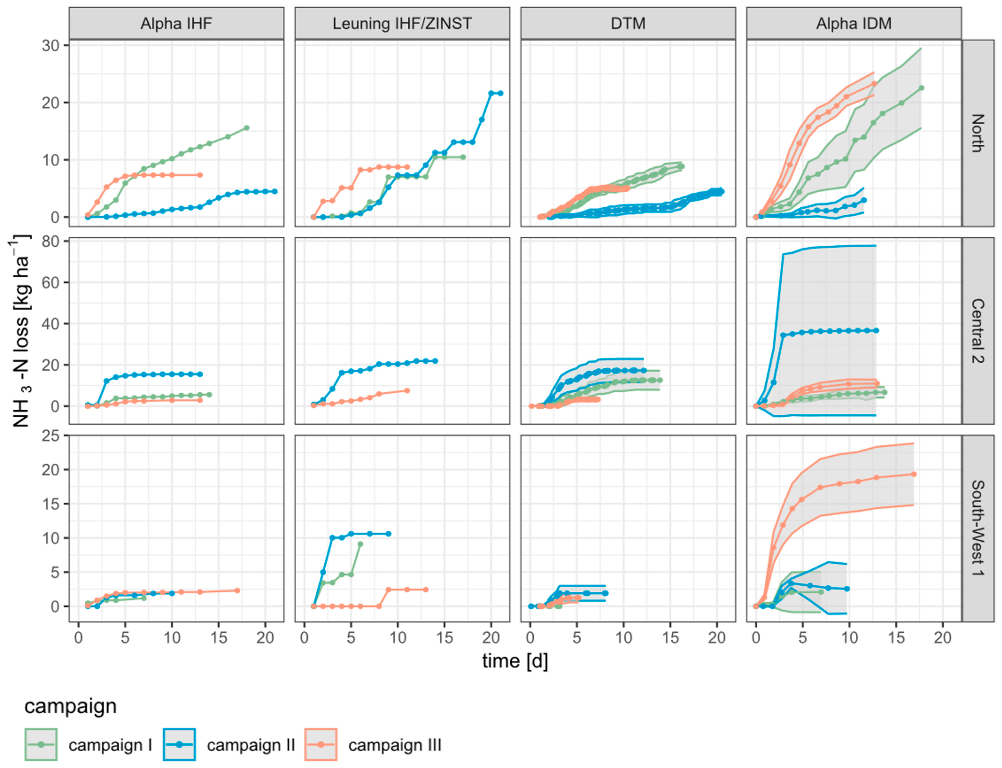
3.1. Cumulative NH₃ Emissions Estimated by Different Methods

In most cases, the cumulative emissions of the measurement campaigns showed a saturation curve after the application of urea (Figure 1; three exemplary locations: North, Central 2 and South-West 1). While the measured cumulative emission curves of the individual campaigns generally agree between DTM and Alpha IHF, the processes determined with Leuning IHF/ZINST and Alpha IDM appear to deviate more strongly. At location North, NH₃ emissions lasted longer in contrast to location South-West 1. At location Central 2, a sharp increase in emission losses in the first four days occurred. This kinetic was recorded consistently with all methods, but with IDM, it was recorded at an upwardly deviating level. The median of the cumulative NH₃ emissions of the 18 measurement campaigns was 3.27 kg N ha⁻¹ (mean 5.97 kg N ha⁻¹).The trials in Central 2 had the highest emissions, with a median of 10.9 kg N ha⁻¹ (mean 12.8 kg N ha⁻¹), despite featuring the lowest application rate (50, 50 and 45 kg N ha⁻¹). Other than differences between locations, seasonal differences between campaigns show an influence on NH₃ emissions. Emissions were highest in the first campaign, with a median of 7.2 kg N ha⁻¹ (mean 8.07 kg N ha⁻¹). The median of the cumulative NH₃ emissions detected with Alpha IHF was 2.57 kg N ha⁻¹ (mean 5.12 kg N ha⁻¹), and with DTM, it was 2.38 kg N ha⁻¹ (mean 4.05 kg N ha⁻¹).

3.2. Comparison of Cumulative NH₃ Emissions

The differences in cumulative NH₃ emissions detected by the reference Alpha IHF compared to the two small-plot methods and the Leuning IHF/ZINST are shown in Figure 2. Across all locations and campaigns, higher deviations were detected on average with Alpha IDM (median 6.45 kg N ha⁻¹, mean 8.53 kg N ha⁻¹) compared to Alpha IHF. For DTM, the deviation of losses had a median of −0.24 kg N ha⁻¹ (mean −0.45 kg N ha⁻¹), showing an underestimation of NH₃ losses, and for Leuning IHF/ZINST, on large plots, a median of 1.93 kg N ha⁻¹ (mean 3.19 kg N ha⁻¹) was observed. After the correction of the Alpha IDM values, the deviation was smaller and in the range of the second micrometeorological method Leuning (IHF/ZINST), with a median of 1.03 kg N ha⁻¹ (mean 2.24 kg N ha⁻¹) (Figure 2).

The cumulative losses of the two small-plot methods, DTM and Alpha IDM, and the Leuning IHF/ZINST method are related to the reference method Alpha IHF in scatterplots (Figure 3).

The cumulative losses of the DTM and Alpha IHF showed high agreement, especially in the low measuring range <5 kg N ha⁻¹ (Figure 3a). With a value of 11% (

Table 3. Comparison of the reference method Alpha IHF with (a) IHF/ZINST with Leuning sampler, (b) the DTM and (c) Alpha sampler used in the small plots by different criteria: the relative root mean squared error (rRMSE) and the mean bias error (MBE). Wind speed and temperature measured at 2 m.

Method	rRMSE [%]	MBE [kg N ha−1]	With Posterior Correction
Alpha IHF ~ DTM	10.68	−0.43	No
Alpha IHF ~ Alpha IDM	39.78	+8.53	No
Alpha IHF ~ Alpha IDM corr. correction factor of 0.27: WS (2 m) <2.1 m s−1 ᴧ temp (2 m) >10 °C no correction: WS (2 m) >2.1 m s−1 ᴠ temp (2 m) <10 °C	19.63	+2.24	Yes
Alpha IHF ~ Leuning IHF/ZINST	20.95	+3.19	No

), the rRMSE is ranked into the excellent range according to the quality classes selected in this study. On the other hand, the cumulative losses of Alpha IDM and Alpha IHF show low agreement, with an rRMSE of 40%. The Alpha IDM method significantly overestimated NH₃ emissions. The Leuning IHF/ZINST method tended to detect higher emissions, but with an rRMSE of 21%, it is ranked in the acceptable evaluation limit.

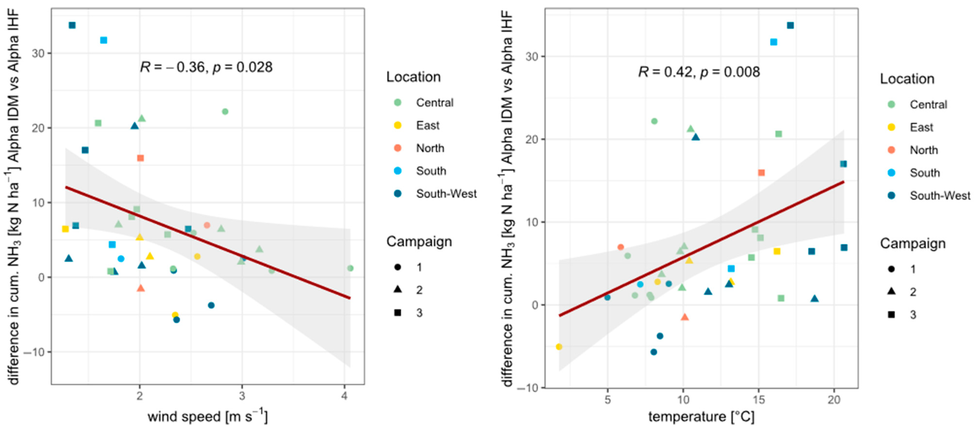
3.3. Correlating Deviation of Cumulative NH₃ Emissions of Alpha IDM from Reference Alpha IHF Method with Environmental Factors

Figure 3b shows higher deviations for Alpha IHF regardless of location. The analysis of various soil parameters (e.g., cation exchange capacity or sand content) showed no correlation with this deviation. The correlation analysis revealed standardized wind and air temperature as the meteorological parameters with the strongest influence on the detected NH₃ loss differences between Alpha IHF and Alpha IDM (Figure 4). This was initially demonstrated using the data set for the 18 trials examined in this study and subsequently verified using a further test data set from 2023 (n = 20 trials, Table S3) using wind speed, temperature and the differences in loss between Alpha IHF and Alpha IDM, respectively (Table S4). The NH₃ loss differences tended to be higher in domains with low wind speeds and high temperatures occurring in fertilization campaign three, while the differences tended to be small at higher wind speeds and temperatures below 10 °C (Figure 4). The negative correlation (R = −0.36) between standardized wind and NH₃ loss difference indicates that NH₃ loss differences are significantly lower under windy conditions (p = 0.028). Consequently, emissions are overestimated at low wind speeds (Figure 4 left). A positive correlation (R = 0.42, p = 0.008) was observed between temperature and NH₃ loss difference (Figure 4 right).

These correlations are based on both data sets for the years 2021 to 2023. For the data set presented in this study, the two concomitant criteria, average wind speed <2.1 m s⁻¹ ∧ average temperature >10 °C, over a whole measurement campaign were identified for the correction of cumulative emissions with a factor of 0.27. This factor is derived from the correlation between Alpha IHF and Alpha IDM (Figure 3b) using the reciprocal of the slope of the regression line. Applying this correction, the rRMSE is reduced to 19.6% and the MBE to +2.2 kg N ha⁻¹, i.e., to a similar acceptable deviation range compared to the Leuning IHF/ZINST (Table 3). The resulting rRMSE for the validation data set (2023, n = 20) after correction is 9.0%, with an MBE of +1.0 kg ha⁻¹, and for all trials from 2021 to 2023 (n = 38), the resulting rRMSE is 10.3% and the MBE is + 1.6 kg ha⁻¹ (Figure 5, Table S4).

4. Discussion

This study presents a data set of 18 measurement campaigns in winter wheat across Germany. Four measurement techniques were used to measure NH₃ emissions from urea, two applied on large plots and two in a small-scale multiplot design. Alpha sampler with IDM was used for the first time in such an experimental design, and Alpha IHF was set as reference method. Results from NH₃ emission studies are often biased due the research group conducting the experiment and the measurement method used [28]. This centrally coordinated study covering five sites in Germany provides a unique and extensive data set to compare and evaluate the applied methods. Scale effects due to the size of the measurement plots are debated but not discussed in the present study.

4.1. Alpha IDM in Small Plots

The initial hypothesis (b) expecting the Alpha IDM approach to provide higher agreement with the Alpha IHF than DTM was not confirmed. Other studies have shown a relative difference in cumulative emissions of 6–28% for IHF, ZINST and IDM/bLS compared to the average emissions assessed by micrometeorological methods [54]. Within the different concentration measurement methods used with bLS, differences of 1–13% in applied total ammoniacal nitrogen (TAN) were found [28]. In this study, a high rRMSE of 39.78% and an MBA of +8.5 kg N ha⁻¹ were determined from uncorrected NH₃ losses obtained by Alpha IDM.

The use of Alpha samplers for IDM with long time intervals reaches the applicability limits of the IDM model, as the parameterization with the Monin–Obukhov similarity theory (MOST) is only valid for shorter time intervals [55]. The assumption of stationarity within averaging intervals of 24 h is not plausible. Therefore, weather data was used at 30 min intervals. However, there is a distortion of the turbulence parameter due to the long averaging intervals used for the concentrations. This could be a contributing factor to the differences between Alpha IHF and Alpha IDM emissions. This effect could be overcome by a higher temporal resolution, like 3–6 h concentration sampling, with Alpha samplers improving the accuracy of IDM. Due to low sensitivity and limitations in equipment or site availability, this is not always possible. Nevertheless, there is a difference between the IHF and IDM methods. Thus, IHF measures concentration and wind profiles directly from multiple heights within the boundary layer. On the other hand, the IDM method assumes that the wind profile can be based on the application of MOST by the utilization of measurements at a single height while applying similarity relationships. Filtering removes periods with more extreme conditions where the assumptions are more likely to be violated [49]. At the same time, removed data (often from night time) and linear interpolation can lead to overestimation.

Cumulative ammonia emissions obtained by Alpha IDM showed good agreement with the reference for the two first fertilizer application timings across sites and experimental years. The influence of the third split application on deviations from the reference method is shown by the data set, as mostly lower wind speeds and comparatively high temperatures prevail. Therefore, cumulated ammonia emissions obtained by small-plot measurements with IDM require correction with a factor of 0.27 (within the limits for campaign-averaged wind speed <2.1 m s⁻¹ ∧ air temperature >10 °C) to yield an acceptable deviation compared to the Alpha IHF reference. The factors are considered to be the best threshold criteria for identifying the need for correction of cumulated NH₃ emissions by Alpha IDM, while they are not necessarily explanatory for the observed differences. The applicability of the factor may be influenced by site-specific factors. Specific canopy traits, like fully developed winter wheat flag leaf or ear appearance under the specified wind and temperature conditions of the third measurement campaigns, may also account for the higher uncertainties of Alpha IDM and be related to the applied Alpha sampler sampling heights. In addition, while low wind speeds are often found to be critical for micrometeorological flux calculations [45], the use of Pasquill–Gifford classes for characterizing atmospheric stability conditions in inverse dispersion modelling has been found to lead to erroneous results under specific conditions (WindTrax users guide 2024). In future measurements following this approach, atmospheric stability parameters for inverse dispersion modelling should be obtained from 3D sonic wind speed measurements. However, by using the correction factor, hypothesis (a) on the quantitative accuracy of NH₃ loss measurements of Alpha samplers combined with IDM in small plots can be accepted, while improvement in Alpha IDM is still needed and should be investigated. As one approach, conducting measurements at different heights in small plots should also be considered. This could entail a more accurate representation of background concentrations and the possibility to quantify potential cross contamination between plots. An additional circular plot should be included in further trials, if the space is available, e.g., with Alpha IHF as reference, to validate and correct absolute flux estimates obtained by Alpha IDM.

4.2. Dräger Tube Method in Small Plots

The initial hypothesis (b), according to which the DTM was expected to be less consistent with the Alpha IHF compared to the Alpha IDM approach, cannot be confirmed. The DTM shows a high agreement with the Alpha IHF, with an rRMSE of 11% and an MBE of −0.4 kg N ha⁻¹.

Generally, enclosure methods feature critical disadvantages in measuring absolute emissions. They modify the environment of the emitting surface compared to ambient conditions by changing the air flow (e.g., turbulence, wind speed and vertical wind profile), along with precipitation, radiation, temperature and soil conditions [56]. A review of chamber and micrometeorological methods to quantify NH₃ emissions from field=applied fertilizer has concluded that enclosure methods, as well as dynamic chambers like wind tunnels, which proved to be the most suitable technique to mimic wind conditions, are a reliable tool for the relative comparison of emissions [57]. For enclosed methods, a relative difference in cumulative emissions of 41–76% for DTM and wind tunnels compared to the average emissions estimated using micrometeorological methods was reported [54]. Some studies observed close agreement of the DTM to measurements made with IDM on liquid manures [27,53], while others observed the opposite, especially with organic (incorporated) fertilizers, due to the heterogeneity regarding unknown fertilizer quantity, placement and a rather small measurement area [21]. In this study, the agreement between DTM and IDM was closer for the urea fertilizer measurements due to the more evenly distributed application within the area covered by the DTM soil rings. However, the DTM does not integrate over large areas and is therefore not robust to spatial heterogeneity or heterogeneous fertilizers such as slurry [28]. In addition, organic fertilizers can lead to a contamination of the chamber system, which can make reliable measurements challenging [30]. The application error of this study is expected to be small in this measurement, since the urea granules were weighed exactly for the corresponding area of the soil rings. Nevertheless, the measured emissions may differ between methods, as small application heterogeneity in plots due to fertilizer spreaders is not representable in small-chamber measurements on soil rings. The results of the present study have shown that DTM is suitable for quantitative NH₃ emission measurement from urea fertilizer under these specific experimental conditions in comparison to the Alpha IHF reference.

The DTM provides direct spot measurements, measured during daytime, when emissions were expected to be the highest, as the highest temperatures and wind speeds were observed during daytime. Although measurements in the morning and in the evening are connected to lower temperatures and wind speeds, emissions were also detected during that time. As no sampling was carried out at night, the lowest daytime emissions may not have been recorded, which may lead to an overestimation of night time emissions with the DTM. Next to this overestimation, underestimation occurred as well, as the initial flows were measured at specific moments when concentrations were partially below the detection limit of the Dräger tubes [29]. For these cases, accumulating samplers with longer exposure times have a great advantage in terms of detecting low emissions. An underestimation of emissions detected with DTM of 34% of applied TAN in comparison with other measurement methods was also reported by other studies [28]. Due to the low number of measurement points and no continuous measurement, no high short-term emission peaks could be detected. This is more likely to be the case with organic fertilizers for which accumulating samplers with longer exposure times performed better (Alpha IDM).

Overall, measurements with the DTM are difficult, both in the very low range due to the detection limits of the point measurements and also in the high range due to the measurement intervals of the individual measurements. In addition, the amount of work involved in field tests with mineral fertilizers is very high, as the emission process can be long, as shown at location North (Figure 1). NH₃ losses detected with the DTM are reliable when the limits and uncertainties of this method are considered.

4.3. Leuning IHF/ZINST

For hypothesis (c), the results obtained by Leuning sampler IHF/ZINST and the reference Alpha IHF showed an acceptable agreement, as emissions were within the expected range of possible deviations. However, emissions showed a tendency to be overestimated with the IHF Leuning method (MBE of +3.2 kg N ha⁻¹).

Relative standard deviations of 23% and 52% are reported when using IHF between replicate plots [20]. The deviations of the Leuning IHF/ZINST from the Alpha IHF found here are within this range. The data in this study is not based on replications within one trial but on measurements by different research groups at different locations, which can cause higher deviations. The positive bias of the IHF, partly due to the contribution of horizontal turbulent diffusion, can cause a systematic overestimation of 5–20% depending on stability [6]. There are various ways to adjust the profiles. In 2020, a new method was proposed, which decreased overestimated emissions by a relative factor of 10% for 160 experiments [43]. This adjustment was chosen for the Alpha IHF calculations in this study as well. This comparison points out that a similar kind of adjustment procedure for Leuning sampler IHF could also be considered. Overall, the use of Leuning samplers as concentration measurement for IHF should be carefully examined and an alternative concentration measurement method should possibly be used, e.g., Alpha sampler.

4.4. Challenges During Concentration Measurements

The use of Alpha and Leuning samplers requires manual handling in several steps, including preparation, set up, collection and laboratory analysis, during which systematic or random errors can possibly occur. In addition, the general disadvantage of concentration measurements with Leuning samplers is the high laboratory effort due to the complex extraction and long drying steps. Replicates in the field are difficult due to the large area required. Furthermore, it is difficult to ensure rotation while preventing samplers from falling down during strong winds, leading to data loss. The IHF results were more robust than the ZINST results, which are more prone to application errors and data loss due to the small number of samplers. Application of ZINST is clearly restricted by its strict prerequisites, such as deriving the empirical ratio of horizontal flux at ZINST height to the emission rate from the plot with specific size and surface roughness, as well as requiring large uniform fields [21]. The concentrations measured with the Dräger tubes were determined visually through a coloured gradient on the tube, potentially being source of random or systematic errors. While this method requires a lot of fieldwork, it eliminates the need for laboratory measurements, as the results of measurements are directly available.

4.5. Combination of Quantitative Methods with Qualitative Passive Flux Sampler

Absolute emission measurements can be combined with qualitative/semi-quantitative NH₃ concentration measurements using passive samplers like sulfuric acid traps or denuders to assess NH₃ emission in plot experiments with many treatments [21]. Ammonia collected by passive samplers on fertilized small plots is then compared with absolute NH₃ emissions collected on standard plots with known rates of NH₃ to determine a transfer coefficient, which is called the standard comparison method [58,59]. Sulfuric acid traps have also been combined with the DTM as absolute emission measurements, which proved to be reliable in field studies [27] and can be used for determining the quantitative NH₃ losses in field trials with multiple plots. However, the need for a quantitative method that is easy to use and implement in small-plot field trials remains. The DTM has proven to be suitable in this study, but there are clear limitations, and the amount of workload involved makes it difficult to implement in field trials. Quantitative NH₃ losses could be detected by Alpha sampler and the backward Lagrangian stochastic dispersion method within small plots. This approach would not need large additional plot size or electricity nor multiple samplings throughout the day. Nevertheless, as described before, more experiments with the Alpha IDM approach are needed to cover various weather conditions and refine the model and sampling approach for the Alpha IDM.

5. Conclusions

This study compared two small-plot NH₃ measurement approaches to a micrometeorological reference method based on a comprehensive, multi-annual data set collected throughout Germany. To date, this study is the first to provide such a comprehensive comparison between methods and to test passive flux Alpha samplers in combination with inverse dispersion modelling to determine NH₃ emissions from mineral fertilizers on small plots. In addition, two micrometeorological approaches were compared, of which integrated horizontal flux (IHF) measurements employing Alpha samplers were in acceptable agreement with IHF/ZINST using Leuning samplers.

The comparison showed a good agreement of the DTM dynamic chamber method with the reference method Alpha IHF for cumulative emissions from homogeneously surface-applied urea fertilizer. Nevertheless, this method has strong limitations, and its application should be carefully considered, particularly regarding the fertilizer application method and the required fieldwork. With respect to Alpha samplers in combination with inverse dispersion modelling, there was good agreement with the reference for early- and middle-of-spring applications. This method is therefore recommended by the authors. Deviations from the reference, particularly in late-spring applications, were related to specific weather threshold values of average air temperature and wind speed within an experimental campaign. A correction factor was derived, which could be considered for the same weather soil and canopy conditions in future investigations. To ensure reliable measurements with Alpha IDM, further improvements should be considered, such as utilizing multiple measurement heights, concentration measurements at higher time resolution or derivation of atmospheric stability parameters from 3D sonic wind speed measurements.

The results of this study show that quantitative ammonia loss measurements from small-plot measurements are feasible under specific conditions. Therefore, providing a supplementary micrometeorological reference measurement on a larger plot is recommended. This can serve as an additional validation and correction of results obtained in a multiple-small-plot set up until more valid and robust small-plot methods are available.

References

1. Griffith, S.M.; Huang, X.H.; Louie, P.; Yu, J.Z. Characterizing the thermodynamic and chemical composition factors controlling PM 2.5 nitrate: Insights gained from two years of online measurements in Hong Kong. Atmos. Environ. 2015, 122, 864–875. [Google Scholar] [CrossRef]
2. Bergström, A.-K.; Janson, M. Atmospheric nitrogen deposition has caused nitrogen enrichment and eutrophication of lakes in the northern hemisphere. Glob. Chang. Biol. 2006, 12, 635–643. [Google Scholar] [CrossRef]
3. Clark, C.M.; Tilman, D. Loss of plant species after chronic low-level nitrogen deposition to prairie grasslands. Nature 2008, 451, 712–715. [Google Scholar] [CrossRef]
4. Hu, Y.; Flessa, H.; Vos, C.; Fuß, R.; Schmidhalter, U. Successful NH3 abatement policies and regulations in German agriculture. Sci. Total Environ. 2024, 956, 177362. [Google Scholar] [CrossRef]
5. Ni, K.; Pacholski, A.; Kage, H. Ammonia volatilization after application of urea to winter wheat over 3 years affected by novel urease and nitrification inhibitors. Agric. Ecosyst. Environ. 2014, 197, 184–194. [Google Scholar] [CrossRef]
6. Sintermann, J.; Neftel, A.; Ammann, C.; Häni, C.; Hensen, A.; Loubet, B.; Flechard, C.R. Are ammonia emissions from field-applied slurry substantially over-estimated in European emission inventories? Biogeosciences 2012, 9, 1611–1632. [Google Scholar] [CrossRef]
7. NIFLUM–Nitrogen. Flux Method Evaluation–Outcomes and Recommendations of an International Expert Workshop; Umweltbundesamt, Ed.; Umweltbundesamt: Dessau-Roßlau, Germany, 2018; Available online: https://www.umweltbundesamt.de/sites/default/files/medien/1410/publikationen/2018-06-01_texte_44-2018_niflum_0.pdf (accessed on 21 July 2025).
8. Braschkat, J.; Mannheim, T.; Horlacher, D.; Marschner, H. Measurement of ammonia emissions after liquid manure application: I. Construction of a windtunnel system for measurements under field conditions. J. Plant Nutr. Soil 1993, 156, 393–396. [Google Scholar] [CrossRef]
9. Sommer, S.G.; Misselbrook, T.H. A review of ammonia emission measured using wind tunnels compared with micrometeorological techniques. Soil Use Manag. 2016, 32, 101–108. [Google Scholar] [CrossRef]
10. Insausti, M.; Timmis, R.; Kinnersley, R.; Rufino, M.C. Advances in sensing ammonia from agricultural sources. Sci. Total Environ. 2020, 706, 135124. [Google Scholar] [CrossRef]
11. Zhou, M.; Li, T.; Liu, P.; Zhang, S.; Liu, Y.; An, T.; Zhao, H. Real-time on-site monitoring of soil ammonia emissions using membrane permeation-based sensing probe. Environ. Pollut. 2021, 289, 117850. [Google Scholar] [CrossRef]
12. Denmead, O. A mass balance method for non-intrusive measurements of surface-air trace gas exchange. Atmos. Environ. 1998, 32, 3679–3688. [Google Scholar] [CrossRef]
13. Flesch, T.K.; Wilson, J.D.; Harper, L.A.; Crenna, B.P.; Sharpe, R.R. Deducing Ground-to-Air Emissions from Observed Trace Gas Concentrations: A Field Trial. J. Appl. Meteor. 2004, 43, 487–502. [Google Scholar] [CrossRef]
14. Flesch, T.K.; Wilson, J.D.; Yee, E. Backward-Time Lagrangian Stochastic Dispersion Models and Their Application to Estimate Gaseous Emissions. J. Appl. Meteor. 1995, 34, 1320–1332. [Google Scholar] [CrossRef]
15. Sommer, S.G.; McGinn, S.M.; Flesch, T.K. Simple use of the backwards Lagrangian stochastic dispersion technique for measuring ammonia emission from small field-plots. Eur. J. Agron. 2005, 23, 1–7. [Google Scholar] [CrossRef]
16. Herrmann, B.; Jones, S.K.; Fuhrer, J.; Feller, U.; Neftel, A. N budget and NH3 exchange of a grass/clover crop at two levels of N application. Plant Soil 2001, 235, 243–252. [Google Scholar] [CrossRef]
17. Wilson, J.D.; Thurtell, G.W.; Kidd, G.E.; Beauchamp, E.G. Estimation of the rate of gaseous mass transfer from a surface source plot to the atmosphere. Atmos. Environ. (1967) 1982, 16, 1861–1867. [Google Scholar] [CrossRef]
18. Famulari, D.; Fowler, D.; Hargreaves, K.; Milford, C.; Nemitz, E.; Sutton, M.A.; Weston, K. Measuring eddy covariance fluxes of ammonia using tunable diode laser absorption spectroscopy. Water Air Soil Pollut. Focus 2005, 4, 151–158. [Google Scholar] [CrossRef]
19. Ferrara, R.M.; Loubet, B.; Di Tommasi, P.; Bertolini, T.; Magliulo, V.; Cellier, P.; Eugster, W.; Rana, G. Eddy covariance measurement of ammonia fluxes: Comparison of high frequency correction methodologies. Agric. For. Meteorol. 2012, 158–159, 30–42. [Google Scholar] [CrossRef]
20. Misselbrook, T.H.; Nicholson, F.A.; Chambers, B.J.; Johnson, R.A. Measuring ammonia emissions from land applied manure: An intercomparison of commonly used samplers and techniques. Environ. Pollut. 2005, 135, 389–397. [Google Scholar] [CrossRef]
21. Ni, K.; Köster, J.R.; Seidel, A.; Pacholski, A. Field measurement of ammonia emissions after nitrogen fertilization—A comparison between micrometeorological and chamber methods. Eur. J. Agron. 2015, 71, 115–122. [Google Scholar] [CrossRef]
22. Kemmann, B.; Brokötter, J.; Götze, H.; Kelsch, A.; Frößl, J.; Riesch, S.; Heinemann, P.; Kukowski, S.; Pacholski, A.; Flessa, H. Ammonia emissions from urea fertilization—Multi-annual micrometeorological measurements across Germany. Agric. Ecosyst. Environ. 2025, 381, 109416. [Google Scholar] [CrossRef]
23. Engel, R.; Jones, C.; Wallander, R. Ammonia Volatilization from Urea and Mitigation by NBPT following Surface Application to Cold Soils. Soil Sci. Soc. Am. J. 2011, 75, 2348–2357. [Google Scholar] [CrossRef]
24. White, R.E.; Cai, G.; Chen, D.; Fan, X.H.; Pacholski, A.; Zhu, Z.L.; Ding, H. Gaseous nitrogen losses from urea applied to maize on a calcareous fluvo-aquic soil in the North China Plain. Soil Res. 2002, 40, 737. [Google Scholar] [CrossRef]
25. Roelcke, M.; Li, S.X.; Tian, X.H.; Gao, Y.J.; Richter, J. In situ comparisons of ammonia volatilization from N fertilizers in Chinese loess soils. Nutr. Cycl. Agroecosyst. 2002, 62, 73–88. [Google Scholar] [CrossRef]
26. Pacholski, A.; Cai, G.; Nieder, R.; Richter, J.; Fan, X.; Zhu, Z.; Roelcke, M. Calibration of a simple method for determining ammonia volatilization in the field—Comparative measurements in Henan Province, China. Nutr. Cycl. Agroecosyst. 2006, 74, 259–273. [Google Scholar] [CrossRef]
27. Gericke, D.; Pacholski, A.; Kage, H. Measurement of ammonia emissions in multi-plot field experiments. Biosyst. Eng. 2011, 108, 164–173. [Google Scholar] [CrossRef]
28. Kamp, J.N.; Hafner, S.D.; Huijsmans, J.; van Boheemen, K.; Götze, H.; Pacholski, A.; Pedersen, J. Comparison of two micrometeorological and three enclosure methods for measuring ammonia emission after slurry application in two field experiments. Agric. For. Meteorol. 2024, 354, 110077. [Google Scholar] [CrossRef]
29. Kelsch, A.; Claß, M.; Brüggemann, N. Accuracy and sensitivity of NH3 measurements using the Dräger Tube Method. Atmos. Meas. Tech. 2025, 18, 1519–1535. [Google Scholar] [CrossRef]
30. Huf, M.T.; Olfs, H.-W. Evaluation of the Dynamic Tube Method for Measuring Ammonia Emissions after Liquid Manure Application. Agriculture 2023, 13, 1217. [Google Scholar] [CrossRef]
31. Huf, M.T.; Reinsch, T.; Kluß, C.; Essich, C.; Ruser, R.; Buchen-Tschiskale, C.; Pacholski, A.; Flessa, H.; Olfs, H.-W. Evaluation of calibrated passive sampling for quantifying ammonia emissions in multi-plot field trials with slurry application. J. Plant Nutr. Soil Sci. 2023, 186, 451–463. [Google Scholar] [CrossRef]
32. Tang, Y.S.; Cape, J.N.; Sutton, M.A. Development and Types of Passive Samplers for Monitoring Atmospheric NO2 and NH3 Concentrations. Sci. World J. 2001, 1, 513–529. [Google Scholar] [CrossRef]
33. Loubet, B.; Carozzi, M.; Voylokov, P.; Cohan, J.-P.; Trochard, R.; Génermont, S. Evaluation of a new inference method for estimating ammonia volatilisation from multiple agronomic plots. Biogeosciences 2018, 15, 3439–3460. [Google Scholar] [CrossRef]
34. Nikolajsen, M.T.; Pacholski, A.S.; Sommer, S.G. Urea Ammonium Nitrate Solution Treated with Inhibitor Technology: Effects on Ammonia Emission Reduction, Wheat Yield, and Inorganic N in Soil. Agronomy 2020, 10, 161. [Google Scholar] [CrossRef]
35. Martin, N.A.; Ferracci, V.; Cassidy, N.; Hook, J.; Battersby, R.M.; di Meane, E.A.; Tang, Y.S.; Stephens, A.C.; Leeson, S.R.; Jones, M.R.; et al. Validation of ammonia diffusive and pumped samplers in a controlled atmosphere test facility using traceable Primary Standard Gas Mixtures. Atmos. Environ. 2019, 199, 453–462. [Google Scholar] [CrossRef]
36. Carozzi, M.; Ferrara, R.M.; Fumagalli, M.; Sanna, M. Field-scale ammonia emissions from surface spreading of dairy slurry in Po Valley. Ital. J. Agrometeorol. 2012, 17, 25–34. [Google Scholar]
37. Carozzi, M.; Loubet, B.; Acutis, M.; Rana, G.; Ferrara, R.M. Inverse dispersion modelling highlights the efficiency of slurry injection to reduce ammonia losses by agriculture in the Po Valley (Italy). Agric. For. Meteorol. 2013, 171–172, 306–318. [Google Scholar] [CrossRef]
38. Kure, J.L.; Krabben, J.; Pedersen, S.V.; Carozzi, M.; Sommer, S.G. An Assessment of Low-Cost Techniques to Measure Ammonia Emission from Multi-Plots: A Case Study with Urea Fertilization. Agronomy 2018, 8, 245. [Google Scholar] [CrossRef]
39. Denmead, O.T.; Simpson, J.R.; Freney, J.R. A Direct Field Measurement of Ammonia Emission After Injection of Anhydrous Ammonia. Soil Sci. Soc. Am. J. 1977, 41, 1001–1004. [Google Scholar] [CrossRef]
40. Leuning, R.; Freney, J.R.; Denmead, O.T.; Simpson, J.R. A sampler for measuring atmospheric ammonia flux. Atmos. Environ. (1967) 1985, 19, 1117–1124. [Google Scholar] [CrossRef]
41. Twigg, M.M.; Berkhout, A.J.C.; Cowan, N.; Crunaire, S.; Dammers, E.; Ebert, V.; Gaudion, V.; Haaima, M.; Häni, C.; John, L.; et al. Intercomparison of in situ measurements of ambient NH3: Instrument performance and application under field conditions. Atmos. Meas. Tech. 2022, 15, 6755–6787. [Google Scholar] [CrossRef]
42. Loubet, B.; Génermont, S.; Ferrara, R.; Bedos, C.; Decuq, C.; Personne, E.; Fanucci, O.; Durand, B.; Rana, G.; Cellier, P. An inverse model to estimate ammonia emissions from fields. Eur. J. Soil Sci. 2010, 61, 793–805. [Google Scholar] [CrossRef]
43. Goedhart, P.W.; Mosquera, J.; Huijsmans, J.F.M. Estimating ammonia emission after field application of manure by the integrated horizontal flux method: A comparison of concentration and wind speed profiles. Soil Use Manag. 2020, 36, 338–350. [Google Scholar] [CrossRef]
44. Flesch, T.K.; Wilson, J.D.; Harper, L.A.; Todd, R.W.; Cole, N.A. Determining ammonia emissions from a cattle feedlot with an inverse dispersion technique. Agric. For. Meteorol. 2007, 144, 139–155. [Google Scholar] [CrossRef]
45. Foken, T. Micrometeorology; Springer: Berlin/Heidelberg, Germany, 2008; ISBN 978-3-540-74666-9. [Google Scholar]
46. Slade, D.H. Meteorology and Atomic Energy; National Technical Information Service: Springfield, VA, USA, 1968. [Google Scholar]
47. Yamartino, R.J. A Comparison of Several “Single-Pass” Estimators of the Standard Deviation of Wind Direction. J. Clim. Appl. Meteor. 1984, 23, 1362–1366. [Google Scholar] [CrossRef]
48. Häni, C.; Flechard, C.; Neftel, A.; Sintermann, J.; Kupper, T. Accounting for Field-Scale Dry Deposition in Backward Lagrangian Stochastic Dispersion Modelling of NH3 Emissions. Atmosphere 2018, 9, 146. [Google Scholar] [CrossRef]
49. Flesch, T.K.; McGinn, S.M.; Chen, D.; Wilson, J.D.; Desjardins, R.L. Data filtering for inverse dispersion emission calculations. Agric. For. Meteorol. 2014, 198–199, 1–6. [Google Scholar] [CrossRef]
50. Bai, M.; Suter, H.; Macdonald, B.; Schwenke, G. Ammonia, methane and nitrous oxide emissions from furrow irrigated cotton crops from two nitrogen fertilisers and application methods. Agric. For. Meteorol. 2021, 303, 108375. [Google Scholar] [CrossRef]
51. Zhao, X.; Huang, Y. A Comparison of Three Gap Filling Techniques for Eddy Covariance Net Carbon Fluxes in Short Vegetation Ecosystems. Adv. Meteorol. 2015, 2015, 1–12. [Google Scholar] [CrossRef]
52. Pacholski, A. Calibrated Passive Sampling--Multi-plot Field Measurements of NH3 Emissions with a Combination of Dynamic Tube Method and Passive Samplers. J. Vis. Exp. 2016, 53273. [Google Scholar] [CrossRef]
53. Quakernack, R.; Pacholski, A.; Techow, A.; Herrmann, A.; Taube, F.; Kage, H. Ammonia volatilization and yield response of energy crops after fertilization with biogas residues in a coastal marsh of Northern Germany. Agric. Ecosyst. Environ. 2012, 160, 66–74. [Google Scholar] [CrossRef]
54. Pedersen, S.V.; di Perta, E.S.; Hafner, S.D.; Pacholski, A.S.; Sommer, S.G. Evaluation of a Simple, Small-Plot Meteorological Technique for Measurement of Ammonia Emission: Feasibility, Costs, and Recommendations. Trans. ASABE 2018, 61, 103–115. [Google Scholar] [CrossRef]
55. Flesch, T.K.; Wilson, J.D.; Harper, L.A.; Crenna, B.P. Estimating gas emissions from a farm with an inverse-dispersion technique. Atmos. Environ. 2005, 39, 4863–4874. [Google Scholar] [CrossRef]
56. Hafner, S.D.; Kamp, J.N.; Pedersen, J. Experimental and model-based comparison of wind tunnel and inverse dispersion model measurement of ammonia emission from field-applied animal slurry. Agric. For. Meteorol. 2024, 344, 109790. [Google Scholar] [CrossRef]
57. Di Perta, E.S.; Fiorentino, N.; Carozzi, M.; Cervelli, E.; Pindozzi, S. A Review of Chamber and Micrometeorological Methods to Quantify NH3 Emissions from Fertilisers Field Application. Int. J. Agron. 2020, 2020, 1–16. [Google Scholar] [CrossRef]
58. Vandré, R.; Kaupenjohann, M. In Situ Measurement of Ammonia Emissions from Organic Fertilizers in Plot Experiments. Soil Sci. Soc. Am. J. 1998, 62, 467–473. [Google Scholar] [CrossRef]
59. Wulf, S.; Maeting, M.; Clemens, J. Application Technique and Slurry Co-Fermentation Effects on Ammonia, Nitrous Oxide, and Methane Emissions after Spreading. J. Environ. Qual. 2002, 31, 1789–1794. [Google Scholar] [CrossRef]
Figure 1. Cumulative NH3-N losses detected by the different methods: IHF with Alpha sampler (n = 1), IHF/ZINST with Leuning (n = 1), the DTM (n = 4) and Alpha sampler IDM (n = 4) in small plots at three exemplary locations, North (top), Central 2 (middle) and South-West 1 (bottom), in 2022 (Table 1). The different colours of the curves represent the campaigns and the grey areas represent the standard deviation for Alpha IDM and DTM.
Environments 12 00255 g001
Figure 2. Difference in cumulative NH3 emissions from urea applied to winter wheat between the reference method Alpha IHF and the two small-plot methods, DTM and Alpha IDM, and the large-plot method, Leuning IHF/ZINST (black), as well as after the application of the correction factor 0.27 on Alpha IDM (green), with the number of replicates in black.
Environments 12 00255 g002
Figure 3. Comparison of the reference method IHF with Alpha sampler with (a) DTM and (b) IDM with Alpha sampler used in the small plots, as well as with (c) IHF/ZINST with Leuning sampler used in the large plots from 18 trials. Error bars represent the standard deviation of 4 replicates (DTM and Alpha IDM). The red dotted line represents the orthogonal regression line equal to the equation shown. The solid grey line represents a 1:1 slope. * standard deviation is 41 kg N ha−1 of Central 2, 2022.
Environments 12 00255 g003
Figure 4. Correlation between the difference in cum. NH3 emissions (Alpha IDM vs. Alpha IHF) and wind speed at the individual sites (left) and temperature at the individual sites (right) with regression lines (95% confidence intervals) and Pearson correlation coefficients from trials over 5 regions in 2021–2023.
Environments 12 00255 g004
Figure 5. Comparison of the reference method IHF with Alpha sampler and IDM with Alpha sampler used in the small plots, applying the Alpha IDM with a correction factor for calculation, with campaign-averaged weather conditions (wind speed <2.1 m s−1 and average temperature >10 °C) from 38 trials in year 2021 to 2023. The solid grey line represents 1:1 slope.
Environments 12 00255 g005