Abstract
Environmental risks often stem from contamination driven by chemical stressors introduced from multiple sources, either geogenic or anthopogenic. Differentiating between anthropogenic chemical anomalies and those inherent to the environment is crucial. This distinction is essential for defining feasible remediation objectives. This study applied univariate and multivariate statistical techniques to analyse geochemical data from over 7000 topsoil samples in Campania (Southern Italy), over an area of approximately 13,600 km2. A key step in the methodology was applying Normal Score Transformation (NST), which stabilized the variance of the dataset, pulling the extreme outliers back to normal ranges, making it more suitable for multivariate analysis. Principal Component Analysis (PCA) was performed, and four components were selected; the spatialization of their scores revealed four primary independent sources controlling geochemical variability across the region. Specifically, two distinct volcanic districts were identified, plus a siliciclastic and an anthropogenic component. The integration of RGB composite maps further refined this differentiation, emphasising the coexistence or the predominance of one component over the other. The methodological approach demonstrated here provides valuable insights for environmental risk assessment and remediation planning in geochemically complex and anthropized regions.
1. Introduction
Soils are the result of physical, chemical, and biological processes affecting rocks and their weathered products. They are the result of natural processes [1,2,3], but also have been widely disturbed by anthropic actions (such as industrial production, motor vehicles mobility, waste disposal and agricultural practices). Soil represents a reservoir of chemical elements and compounds featuring an extreme spatial variability across the whole Earth [4,5]. Defining the distribution of chemical elements and their anomalies, as well as understanding the nature of the factors controlling their spatial variability, is essential for those committed to environmental management, particularly when addressing the effects on ecosystems and living beings to target the development of remedial actions. In this framework, it is crucial to understand the apportionment of inputs [6] to focus on reducing the anthropogenic rather than geogenic contribution. Of course, this latter point is challenging, especially when assessing the environmental status of an anthropized area, where urban and industrial settlements and agricultural practices make the presence of uncontaminated soils relatively uncommon.
Many approaches that assess the entity and origin of elemental enrichments in soil are based on comparing locally observed concentrations with reference levels, such as the average composition of the Earth’s crust, regionally developed background thresholds or local potentially uncontaminated soil. Among these methods, it is worth noting the Enrichment Factor (EF) [7], the Igeo [8], the Contamination Factor (CF) [9], the Pollution Index (PI) [10], and others. Reimann and de Caritat [11] note that the methods listed above are not necessarily capable of discriminating the amount of contamination due to anthropogenic sources, since several natural processes, also occurring at a very local scale, may lead to elevated concentrations of chemical elements in the soil. It follows that the discrimination of natural and anthropogenic contributions to the overall number of chemical elements in soil should follow a more articulate path, possibly focusing on the complexity of the potential sources rather than on the divergence of the measured concentration from the expected one.
Geochemical data often exhibit non-normal distributions, as they present outliers that can strongly influence their distribution; this is due to the complex interplay between multiple sources, such as varying lithological units, anthropogenic inputs, and natural geochemical processes. These diverse origins can lead to skewed or multimodal distributions, challenging the assumptions of traditional statistical methods that rely on normality [12,13,14]. Therefore, normalization methods must be applied. Non-linear transformations are frequently employed in analysing geochemical datasets to account for skewed distributions, reduce the influence of extreme values, and improve the applicability of statistical techniques that assume normality or linear relationships among variables [15]. A variety of normalization techniques have been proposed by several authors, such as the Box–Cox transformation [16,17], the normal score transformation [18], or the log-transformation [19,20,21], even though the results can often be moderately different.
Geochemical datasets derived from environmental studies often feature a multidimensional structure that allows researchers to work on individual variables and consider the simultaneous changes occurring in multiple elements in space and over time, in the case of numerous sampling campaigns. Multivariate analysis (e.g., Factor Analysis, Cluster Analysis, Principal Component Analysis) has proven to be a valuable tool for robustly and consistently investigating geochemical datasets [22,23,24].
Principal Component Analysis (PCA) is a widely used technique that aims to reduce the dimensionality of data by transforming correlated variables into a set of uncorrelated principal components, which capture the underlying structure of the data by representing the relationships among the original variables without redundancy [25]. The interpretability among the variables can be enhanced by applying different rotation methods [26]. Varimax rotation is the most used method, although other methods exist, such as Promax, Oblimin, and Quartimin [27,28]. Varimax operates under the assumption that the resulting components are orthogonal, and thus statistically independent, implying that the loading of a variable on one component does not affect its loadings on the others. This rotation method produces a simpler structure, making it easier to associate element groupings with specific geochemical processes or sources [29,30]. This is particularly useful in geochemical studies, where distinct factor patterns often reflect lithological, anthropogenic, or hydrothermal influences.
Specifically, PCA has been widely applied for geochemical and other types of geoscientific data investigation [31]. Mineral exploration has long used it by determining multi-elemental associations, which could be used as practical markers for mineralized areas [32,33] and to highlight geochemical anomalies related to the geology and mineralization of the underlying bedrock [34]; it also helps identify and distinguish the different origins of specific minerals based on their chemical composition, allowing one to trace the provenance and therefore identify potential hidden mineralized areas [35]. Also, the study of geochemical processes that regulate the compositional evolution of magma has benefited from the application of PCA [36]. In recent studies, the combination of different multivariate statistical methods has proven to be particularly interesting in interpreting and managing different geologic matrices (e.g., hydrogeochemistry, mineralized area) [37,38]. It has also been widely used to examine the spatial distribution of heavy metals in soils [39,40]. In recent decades, PCA has also been successfully used in environmental geochemistry [37,41,42], in studies referring to different spatial scales (from continental to very local scales), to discriminate the contributions proceeding from anthropogenic sources from those of geogenic origin, and to differentiate multiple sources even if they are all dependent on natural processes (e.g., different lithologies) or human actions (e.g., various industrial processes).
While normalization techniques and multivariate statistical tools are commonly used in geochemical studies, their application often varies depending on the scale of analysis, study objectives, and methodological approach. This variability raises a key question: How can a standardized, reproducible, and scalable procedure be developed for applying these tools in complex geological and environmental contexts? Addressing this is essential to improve the comparability and reliability of geochemical analyses across studies.
This work aims to develop a consistent and operationally robust workflow to characterize topsoil geochemical patterns in highly anthropized areas with significant geological variability. The Campania region in southern Italy, with its complex geology and widespread anthropogenic pressure, was selected as an ideal case study for testing the proposed workflow.
2. Materials and Methods
2.1. Study Area
The Campania Region in southern Italy (Figure 1) covers an area of approximately 13,600 km2 and is Italy’s third most populous region, with about 5.6 million inhabitants.
It can be morphologically divided into two main areas. The first is the NW–SE trending Apennine Mountains, which formed during the Cretaceous–Tertiary Alpine orogeny. These mountains consist of NE-verging thrust sheets, resulting from the NE–SW compression caused by the ongoing subduction of the Adriatic and Ionian microplates [43,44]. The Apennines are composed of Mesozoic carbonate rocks and primarily Tertiary siliciclastic rocks, deposited in various tectonic environments. The highest peaks, which reach 1800–2000 m, are composed of carbonate rocks and feature steep slopes with debris flow deposits. Surrounding the mountains are moderately high hilly regions, where siliciclastic rocks, such as siltstones, sandstones, and conglomerates, dominate (Figure 1a).
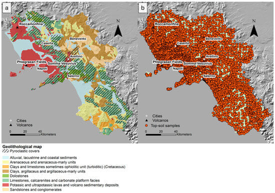
Figure 1.
(a) Geolitholical map modified after Guarino et al. [45]; (b) Map of topsoil sample distribution.
Subsequently, during the Quaternary period, tectonic processes led to faulting along the western side of the Apennine chain, coinciding with the onset of back-arc volcanic activity. This activity began with the formation of the Roccamonfina volcano (700,000 years ago), followed by Ischia Island (150,000 years ago), the Phlegraean Fields (60,000 years ago), and Somma–Vesuvius (25,000 years ago). During this time, large depressional structures were filled with alluvial and volcanic deposits, which are currently found in the main alluvial plains of the Campania and Sele Rivers. The oldest volcanic deposits are associated with the Roccamonfina volcanic complex to the north (Figure 1), where ultrapotassic and potassic lava and pyroclastic rocks were emplaced between 0.6 and 0.1 Ma [46,47]. Most pyroclastic deposits are associated with large ignimbrite eruptions from Mt. Somma–Vesuvius and the Phlegraean Fields (Figure 1a), with the largest ignimbrite event occurring approximately 39,000 years ago [48,49,50]. These eruptions were triggered by fractures resulting from intense block-faulting and rifting on the western side of the Apennines [51]. The alkaline magmatism, characterized by a high potassium content [52,53], is part of the Roman Magmatic Province.
2.2. Soil Sampling and Analyses
The soil sampling was conducted using methodologies established by the Forum of European Geological Surveys (FOREGS), now known as EuroGeoSurveys [54], and the GEMAS (Geochemical Mapping of Agricultural and Grazing Land Soil) programs for regional geochemical mapping [55]. Specifically, subsamples were mixed to obtain a more representative composite sample at each site. The study area was divided into 100 × 100 m grids, with subsamples taken from the four corners and the centre of each grid cell, which were subsequently homogenized into a single composite sample. A total of 7300 samples (5–15 cm) were collected (Figure 1b), with a higher sampling density in urban areas compared to suburban ones, and then transported in polyethylene bags. As a first step, all samples were dried using infrared lamps at a temperature below 35 °C, followed by sieving through a 2 mm mesh. The sieved fractions were then subjected to chemical analysis for 52 elements (Ag, Al, As, Au, B, Ba, Be, Bi, Ca, Cd, Ce, Co, Cr, Cs, Cu, Fe, Ga, Ge, Hf, Hg, In, K, La, Li, Mg, Mn, Mo, Na, Nb, Ni, P, Pb, Pd, Pt, Rb, Re, S, Sb, Sc, Sn, Sr, Te, Th, Ti, Tl, U, V, W, Y, Zn, Zr) using Inductively Coupled Plasma Mass Spectrometry (ICP-MS) and Inductively Coupled Plasma Emission Spectrometry (ICP-ES) at Bureau Veritas (formerly Acme) Analytical Laboratories Ltd. in Vancouver, BC, Canada.
The dataset comprises two subsets of topsoil samples collected as part of two geochemical prospecting projects [56,57]. The total of 7300 samples represents the progressive integration of these subsets over time, reflecting the evolution of the sampling campaign. As the study advanced, the analytical scope was gradually expanded to include additional elements, in line with improvements in laboratory instrumentation and analytical techniques. As a result, the number of samples available for each analyte varies since some elements were introduced into the analysis at later stages.
Reagent blanks, duplicate samples, and certified reference soil verified the precision and accuracy of the analyses. Data quality was assessed using two duplicate pairs, and the results were considered following international standards. Precision was calculated as the Relative Percent Difference (% RPD) based on duplicate sample results, while accuracy was determined from the analyses of replicate standard samples. For the analysed elements, the quality controls were consistent, with a precision and accuracy below 8%. The values below the detection limits (DLs) were replaced by half the DL of the corresponding element, as this provides an approximation without assuming a zero value, which could be incorrect [55]. For more details on RPD and accuracy, see Table 1 in the Results section.

Table 1.
Main statistical indices for the 21 elements in the topsoils of the Campania region. Note: Element concentrations are given in mg/kg, except for Hg (µg/kg).
2.3. Data Preparation and Multivariate Analysis
To mitigate the effects of the non-normality of the geochemical dataset, a transformation was applied to normalize the dataset. One of the most frequently used methods, the Box–Cox transformation, allows one to identify which power transformation can best convert their distribution to a quasi-symmetric one, making the interpretations of the results more straightforward [16]. It is based on applying a parametric power transformation controlled by a lambda (λ) parameter, which varies within a defined range. This normalization also allows for back-transforming the data following statistical analysis. Since normalization was applied, class intervals for the spatial distribution maps were determined based on the median (M) and standard deviation (σ), with threshold values set at M ± 2σ, M ± σ, and M itself. These values were then back-transformed to provide concentrations in their original units (mg/kg), ensuring that the classification remained interpretable in a raw geochemical context. Spatial distribution maps of the raw data concentration were generated using ArcGIS (version 10.8).
A Normal Score Transformation (NST) was also applied to improve its suitability for multivariate statistical analysis. A Kolmogorov–Smirnov (K-S) test was conducted on the transformed dataset to ensure the goodness of normalization by NST. The data transformation, the K-S test, and descriptive statistical analysis were performed using IBM SPSS Statistics 25 and Microsoft Excel, respectively.
Before applying the multivariate approach, the Kaiser–Meyer–Olkin (KMO) test was determined for each variable to assess the data’s adequacy for dimensionality reduction. The KMO test measures the proportion of variance among variables that may be due to common variance, thereby indicating the suitability of the dataset for multivariate analysis. A KMO value of 0.5 or above is considered acceptable for proceeding with the analysis [58,59].
A Principal Component Analysis was performed in R software (ver. 2022.07.2 Build 576) on a subset of 5864 samples, as they represent the common dataset for which all analytes were available. A Varimax rotation was applied to facilitate the interpretation of the results, as it is an orthogonal rotation that minimizes the number of variables with high loadings on each component. Only variables with loadings greater than 0.6 were considered when identifying the element associations for each principal component, to improve the interpretability of the results and minimize the influence of weaker correlations. The components obtained were studied and interpreted following their presumed origin (natural, anthropogenic or mixed). The derived component scores were plotted for the spatial distribution maps in ArcGIS (ver. 10.8) and were interpolated with Inverse Distance Weighted (IDW).
3. Results
In this study, 21 of the 53 elements were selected for further analysis: As, Be, Bi, Cd, Co, Cr, Cu, Hg, Ni, Mn, Mo, Pb, Sb, Sn, Sr, Th, Tl, U, V, and Zn. The selected elements include Potentially Toxic Elements (PTEs), which are known for their environmental and health risks due to their toxicity and potential to bioaccumulate. Additionally, elements such as Be, Bi, Sr, and Th were chosen for their geochemical importance, as they reflect the region’s complex geology [56,60,61].
Table 1 summarizes the basic statistics for the 21 selected elements in the topsoils of the Campania region. All the elements exhibit a significant difference between the minimum and maximum values, indicating substantial variation. Potential outliers could occur, considering the high coefficient of variation (CV) and the considerable discrepancies between the 95th percentile and the maximum values. The significance (ρ < 0.05) of the Kolmogorov–Smirnov test (K-S test), as well as the values of skewness and kurtosis, indicate the non-normality of the raw data for all the considered variables (Supplementary Material, Figure S1). However, the data pass the K-S test after the Normal Score transformation (ρ > 0.05), yielding a symmetrical distribution, as shown in Supplementary Material (Figure S2).
3.1. Raw Data Distribution
The study area’s spatial distribution of element concentrations reflects a complex interaction of geological, volcanic, and anthropogenic factors (Figure 2 and Figure 3).
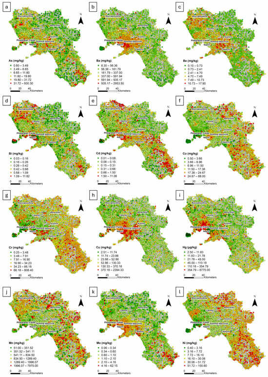
Figure 2.
Raw distribution maps of (a) As; (b) Ba; (c) Be; (d) Bi; (e) Cd; (f) Co; (g) Cr; (h) Cu; (i) Hg; (j) Mn; (k) Mo; (l) Ni. Six class intervals were defined using the median (M) and standard deviation (σ) values, as follows: <(M − 2σ); (M − 2σ) − (M − 1σ); (M − 1σ) − (M + 1σ); (M + 1σ) − (M + 2σ); >(M + 2σ).
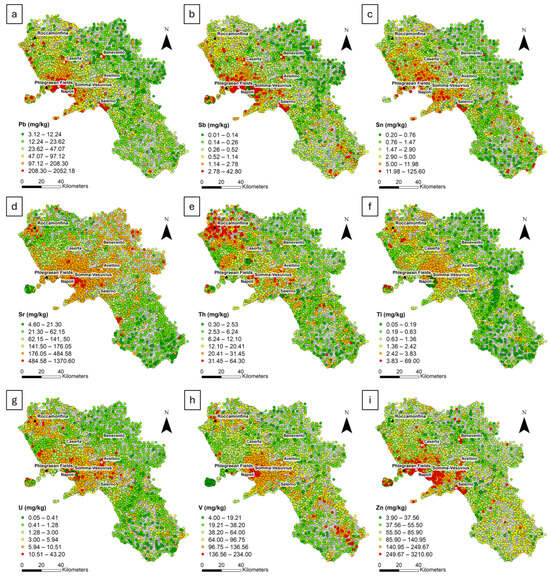
Figure 3.
Raw distribution maps of (a) Pb; (b) Sb; (c) Sn; (d) Sr; (e) Th; (f) Tl; (g) U; (h) V; (i) Zn. Six class intervals were defined using the median (M) and standard deviation (σ) values, as follows: <(M − 2σ); (M − 2σ) − (M − 1σ); (M − 1σ) − (M + 1σ); (M + 1σ) − (M + 2σ); >(M + 2σ).
Arsenic, Bi, Be, and Mo are clearly associated with volcanic areas and carbonate massifs characterized by pyroclastic covers. For As, medium to high values (19.80–930.30 mg/kg) are localized in volcanic regions and on massifs affected by deposits from the Campanian Ignimbrite eruption. Similarly, Bi, with a range of 0.03–11.82 mg/kg, shows a comparable distribution, presenting medium-high values (0.68–11.82 mg/kg) in these same areas. The medium to high values for Be (7.49–17.90 mg/kg) and Mo (2.10–62.15 mg/kg) are also concentrated in volcanic areas and along the Apennine chain, with Mo reaching its highest values (>4.16 mg/kg) in the southern part of the territory. Thorium, with medium values (20.41–31.45 mg/kg), is distributed across carbonate massifs and volcanic areas, with the Roccamonfina area showing the highest concentrations (>31.45 mg/kg). Uranium follows a similar pattern, exhibiting medium to high values (5.94–43.20 mg/kg) in volcanic and carbonate areas and medium values (3–5.94 mg/kg) in the surrounding zones, which further decrease in the peripheral regions.
Elements such as Co, Ni, and Mn exhibit a similar distribution, with medium to high concentrations localized in the southern and northeastern sectors. For cobalt (17.38–88 mg/kg) and Ni (30.06–155.60 mg/kg), medium to high concentrations are found in the same areas, while Mn (1289.40–7975 mg/kg) exhibits a gradient that decreases toward the western coast. Chromium exhibits a similar behaviour, with medium concentrations (34.23–66.18 mg/kg) distributed in the southeastern sectors and some high concentrations (>66.18 mg/kg) in the southern area of Somma–Vesuvius.
Barium, Sr, and Cu are strongly associated with volcanic areas and carbonate massifs. Barium, with concentrations reaching 2953.50 mg/kg, shows medium to high values (591.94–935.17 mg/kg) in the Somma–Vesuvius and Roccamonfina regions, while Sr (176.05–1370.60 mg/kg) is primarily concentrated in these same volcanic areas and the northeastern part of the region. Similarly, medium to high Cu concentrations (130.33–370.18 mg/kg) are distributed around the Somma–Vesuvius area, with higher values (>370.18 mg/kg) localized in two samples along the eastern border of the territory.
Lead, Sb, Sn, and Zn show a distribution associated with major urban centres and anthropogenic activities. Lead (97.12–208.30 mg/kg) and Sb (1.14–2.78 mg/kg) reveal medium to high concentrations in the main cities, with some lead samples reaching very high values (>208.30 mg/kg). Tin (5–125.60 mg/kg) is also distributed in urban centres and the northern and southeastern sectors, while Zn (140.95–249.67 mg/kg) is predominantly located in urban areas, with specific zones showing concentrations exceeding 249.67 mg/kg.
Mercury, Cd, and Tl correlate with urban centres and internal areas. Mercury shows medium to high concentrations (110.18–6775 µg/kg) in Naples, Salerno, and some internal regions, whereas Cd, with medium values (0.66–1.50 mg/kg), is localized near major urban centres and in the southern part of the territory, with high concentrations (>1.50 mg/kg) in the northern sector.
Thallium and V are predominantly distributed in volcanic areas and carbonate massifs. Thallium (3.83–69 mg/kg) and V (136.56–234 mg/kg) exhibit higher concentrations in volcanic areas and across the massifs with pyroclastic covers, with medium values gradually decreasing toward peripheral zones.
3.2. Spatializing Principal Component Scores
The KMO test yielded an overall value of 0.89, indicating that the dataset had a strong underlying structure, with variables sharing a high degree of common variance. Thus, a Principal Component Analysis was highly appropriate, with results likely reflecting real latent patterns. The proper number of components was determined based on eigenvalues greater than 1 [62].
Table 2 presents the PCA results, including loadings, eigenvalues, the percentage of variance, and the cumulative proportion.
Table 2.
Loadings, eigenvalues, variance, and cumulative variance percentage for PCA. Note: PCA loadings values higher than 0.6 are in bold.
The first four Principal Components, PC1, PC2, PC3, and PC4, were selected based on eigenvalues greater than 1, accounting for a total explained variance of 77.2%.
The PC1 (Figure 4a), which includes the associations Th, Be, As, Tl, U, V, and Bi, accounts for 42.5% of the total variance. The score values greater than 1 correspond to the main volcanic district of Roccamonfina, the Volturno Plain, as well as the main carbonate massifs of the region, and gradually decrease to scores between 0.5 and 1.0. Scores less than −0.5 are prevalent in the northeastern and southwestern sectors of the region, where siliciclastic units are present. The remaining territory exhibits no significant scores, ranging from −0.5 to 0.5.
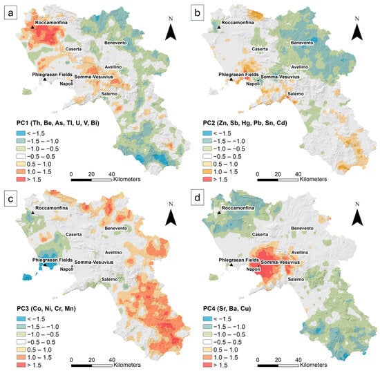
Figure 4.
IDW interpolated distribution maps showing component scores for (a) PC1, (b) PC2, (c) PC3, (d) PC4.
The PC2 (Figure 4b) associated with Sn, Pb, Sb, Cd, Zn and Hg accounts for 15.7% of the total variance. Scores greater than 1.0 are observed across the main urban centres of the region, primarily in the cities of Naples and Salerno, as well as in the southern sector. Values between −0.5 and 0.5 are prevalent throughout most of the territory, while negative scores less than −1.0 characterize the eastern part of the area.
PC3 (Figure 4c), characterized by the association of Mn, Ni, Cr, and Co, accounts for 10.1% of the total variance. Scores greater than 1.0 are located along the western side of the region and in the southern sector, corresponding to the areas of the siliciclastic units. The remaining part of the territory is characterized by values between −0.5 and 0.5, with negative values (<−1.0) primarily located across the Phlegraean Fields and Ischia Island.
PC4 (Figure 4d), which includes the associations Sr, Ba, and Cu, accounts for 8.8% of the total variance. Scores greater than 1.0 are specifically located in correspondence with the Somma–Vesuvius area, gradually decreasing to values between 0.5 and 1 in the surrounding area. Negative scores (<−1.0) are located in the north and south sectors of the region, while the remaining parts are characterized by non-significant values, ranging between −0.5 and 0.5.
4. Discussion
4.1. Data Distribution and Visualization
The analysed data exhibited a lognormal distribution, a typical behaviour for geochemical variables due to the multiple geological and environmental processes governing their distribution. To ensure the applicability of statistical methods that assume a normal distribution, a normal score transformation (NST) was applied, resulting in a normally distributed dataset. NST is an effective method used to convert the original distribution of the data into a standard normal distribution by ranking data values according to their corresponding ranks in a normal distribution, from lowest to highest. Compared to another normalization approach (e.g., Box–Cox), its advantage was the non-linear score transformation, which improved the dataset for variance analysis. The rank-based transformation reduces the influence of outliers by assigning them less weight relative to central observations. As a result, the distribution of transformed data is very close to the Gaussian distribution (see Supplementary Material, Figure S2) rather than other transformation approaches.
The spatial distribution maps of raw geochemical data provide a direct visualization of element concentration patterns across the study area, revealing distinct spatial trends and variability. The observed distributions reflect the influence of geological and potentially anthropogenic factors, with specific regions showing enrichment or depletion for certain elements. The concentration ranges help to delineate geochemical anomalies and assess potential controlling processes. Since these maps are essential for understanding the trends in raw data, integrating them with further statistical analyses enables a more comprehensive interpretation of the underlying mechanisms influencing element dispersion. In fact, despite the complex processes involved in soil formation, which result in significant overlaps in soil chemical composition, the influence of parent material is distinct and identifiable.
4.2. Spatializing Principal Component Scores
The entire dataset was reduced to components using PCA to understand the different controlling factors affecting the distribution of elements in the topsoils. This approach was selected due to its methodological robustness, interpretability, and computational efficiency. In addition to highlighting the associations among elements along independent components, often corresponding to distinct geochemical sources, PCA enables the analysis of score distributions, thereby allowing for a more precise spatial delineation of these sources [11,55]. The Varimax rotation was applied to enhance the loadings of variables with high covariance (e.g., variables associated with anthropogenic factors).
Given the elements’ association with PC1 and their localization, it seems reflective of the potassic and ultrapotassic rocks from which soils developed. The high scores show a good correspondence with the main volcanic districts and the carbonate massifs, characterized by widespread pyroclastic coverings from the Ignimbrite Campana eruptions. This also applies across the Sorrento Peninsula and the eastern sector of Somma-Vesuvius, where the volcanic products of the Ottaviano (8000 BCE) and Avellino (3800 BCE) eruptions are present [63,64,65] (Figure 4a).
PC2 may reflect the effects of human activities, as displayed by the good matching between high scores and urban centres [61,66]. This also applies to the southern part of the region, where an extensive road network for internal and external regional connectivity is present (Figure 4b).
PC3 may be linked to clay-dominant soils developed from siliciclastic deposits. In particular, Mn plays a crucial role as it determines the co-precipitation of other elements, such as Ni, Co, and Cr [67,68]. Indeed, there is a good spatial correspondence between high scores and the outcrop of clay and marly units (Figure 1a).
PC4, with the association of Ba, Cu, and Sr, seems to reflect the volcanic origin of the soils developed by the younger Vesuvian products, which are enriched by these elements. As suggested by Savelli [69], this enrichment could be linked to processes such as the gravitational separation of augite from the magma, as well as other factors, including gas transport and carbonate assimilation (Figure 4d).
It is worth noting that neither of the two components associated with volcanic processes (PC1 and PC4) seem to be representative of the geochemical signature of the Ischia and Phlegraean Fields volcanic districts. However, both areas exhibit negative scores on PC3, indicating that the weathering of siliciclastic deposits is not predominant. It may suggest that, although the two districts exhibit similar geochemical behaviour, they remain distinct entities compared to the Roccamonfina and Somma–Vesuvius volcanic complexes.
Previous studies of the Campania region [61,70] identified three primary geochemical sources: one associated with volcanic origin, one with siliciclastic material, and one with anthropogenic activities. However, none of them had ever identified the recent products of Somma–Vesuvius as a distinct entity, separate from the other volcanic products of the area, in a single component.
4.3. RGB Colour Composite Map
The colour composite maps (Figure 5) confirmed all the above considerations, which were developed to provide an integrated representation of PC1, PC2, PC3, and PC4.
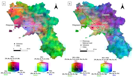
Figure 5.
Colour composite map of (a) PC1, PC3, and PC4; (b) PC1 + PC4, PC2, and PC3.
This chromatic approach enables the differentiation and highlighting of the distinct geochemical signatures of the components, offering a synoptic view of the natural processes occurring in the area and potential zones of overlap in geochemical signals [70,71]. Looking at Figure 5a, the PC1 signal (in red), mainly associated with soils developed from volcanic products of Roccamonfina, is prominently represented by the presence of the colour red, still in correspondence with the volcano. The PC4 signal (in blue), attributed to soils originating from the recent products of the Somma–Vesuvius complex, is limited to its volcano’s district, as shown in Figure 4d. The Phlegraean Fields area is marked by a purple hue, resulting from the overlap of the red and blue bands, which reflects the overlapping geochemical signals associated with PC1 and PC4, thereby making the signal in the Phlegraean area more discernible. The PC3 signal (green), associated with the geochemical signature of the soils derived from siliciclastic units, is predominantly localized across the southern and northwestern sectors. This would confirm again the strong correlation of elements such as Co, Mn, Ni, and Cr with these basin deposits.
The two components associated with volcanic activity (PC1 and PC4) were summed to compare the anthropogenic and natural components. Figure 5b represents the composition of the components PC1 + PC4 (red), PC2 (green), and PC3 (blue), which helps identify interactions between anthropic and natural processes. There is a clear overlap between anthropogenic and natural components in the southern sector of the Somma–Vesuvius area, specifically in the Sarno River basin, an area that has historically been subjected to significant environmental pressure [72,73]. The PC2 also appears to dominate the area between Naples and Caserta, where a dense road network, industrial activities, and agricultural practices occur.
The same pattern is observed in the southern sector, where shades spanning from light blue to light green indicate a co-dominance of siliciclastic and anthropogenic influences. The strong PC2 signal appears to follow principal road axes, including the regional section of the A2 motorway, which represents the primary road connection to the southernmost part of Italy.
5. Conclusions
This study investigated the origin of geochemical variation and the controlling factors of 21 variables in soils of a highly anthropized area characterized by complex geological variability, such as the Campania region. The applied technical operating workflow, incorporating a normal score transformation (NST) and principal component analysis (PCA), revealed different controlling factors influencing the distribution of the selected elements, particularly in volcanic and siliciclastic units. Soils originating from volcanic lithologies, primarily from Roccamonfina, are associated with high concentrations of Th, Be, As, Tl, U, V, and Bi. In contrast, soils formed from volcanic products from Somma–Vesuvius are associated with high concentrations of Ba, Cu, and Sr. High concentrations of Mn, Ni, Cr, and Co are associated with soils derived from siliciclastic units. In addition, high concentrations of Sn, Pb, Sb, Cd, Zn, and Hg are associated with the anthropogenic pressure of the main urban centres and infrastructures across the territory.
The key difference between this research and previous studies in the area is an additional component explicitly related to the Somma–Vesuvius area. This distinction has allowed the discrimination of different geochemical fingerprints from different volcanic districts, emphasizing the independence of variability sources, which previous studies have not achieved. This improvement is likely due to the chosen normalization method, NST, which optimizes the dataset for further statistical processing to extract more detailed geochemical information, in contrast to previous work that tended to group all volcanic-related elements into a single component. Future studies, with more in-depth analyses, could also aim to identify the characteristic element associations of Phlegraean and Ischia’s volcanic products.
The present study proposed a streamlined operational workflow for geochemical data analysis in complex environmental contexts. This workflow is statistically supported by applying the Kolmogorov–Smirnov (KS) and Kaiser–Meyer–Olkin (KMO) tests to ensure the dataset’s normal distribution and its adequacy for multivariate analysis. Its reproducibility and scalability make it particularly valuable for large-scale regional assessments and local studies, provided each step is rigorously followed under similar data conditions.
These findings underscored the effectiveness of multivariate analysis, particularly PCA, in discriminating between geogenic and anthropogenic processes and further distinguishing among various anthropogenic sources. This methodological approach offers valuable insights for managing environmental risks and prioritizing remediation efforts.
Supplementary Materials
The following supporting information can be downloaded at: https://www.mdpi.com/article/10.3390/environments12050163/s1, Figure S1: Raw data distribution plots of the studied elements; Figure S2: Normal score transformed data distribution plots of the studie elements.
Author Contributions
Conceptualisation, A.I., C.Z. and S.A.; software, A.I.; validation, S.D.; formal analysis, A.I.; investigation, A.I. and S.D.; methodology, A.I., C.Z. and S.A.; resources, S.A.; data curation, A.I. and S.D.; writing—original draft preparation, A.I. and S.D.; writing—review and editing, S.A., L.R.P. and A.D.F.; visualisation, A.I.; supervision, S.A. and C.Z.; project administration, S.A.; funding acquisition, S.A. All authors have read and agreed to the published version of the manuscript.
Funding
This study was carried out within the RETURN Extended Partnership and received funding from the European Union Next-GenerationEU (National Recovery and Resilience Plan—NRRP, Mission 4, Component 2, Investment 1.3—D.D. 1243 2/8/2022, PE0000005).
Data Availability Statement
The datasets used in this article are not readily available because the data are part of an ongoing study. Requests to access the datasets should be directed to Stefano Albanese (stefano.albanese@unina.it).
Conflicts of Interest
The authors declare no conflicts of interest.
Abbreviations
The following abbreviations are used in this manuscript:
| IDW | Inverse Distance Weighted |
| K-S | Kolmogorov–Smirnov |
| KMO | Kaiser–Meyer–Olkin |
| M | Median |
| NST | Normal score transformation |
| PCA | Principal component analysis |
References
- Tipping, E.; Lawlor, A.J.; Lofts, S.; Shotbolt, L. Simulating the Long-Term Chemistry of an Upland UK Catchment: Heavy Metals. Environ. Pollut. 2006, 141, 139–150. [Google Scholar] [CrossRef] [PubMed]
- Birke, M.; Reimann, C.; Rauch, U.; De Vivo, B.; Halamić, J.; Klos, V.; Gosar, M.; Ladenberger, A. Distribution of Cadmium in European Agricultural and Grazing Land Soil. In Chemistry of Europe’s Agricultural Soils—Part B: General Background Information and Further Analysis; Geologische Bundesanstalt für Geowissenschaften und Rohstoffe (BGR): Hannover, Germany, 2014; pp. 89–116. [Google Scholar]
- Zhang, C.; Fay, D.; McGrath, D.; Grennan, E.; Carton, O.T. Statistical Analyses of Geochemical Variables in Soils of Ireland. Geoderma 2008, 146, 378–390. [Google Scholar] [CrossRef]
- Rodrigues, S.; Urquhart, G.; Hossack, I.; Pereira, M.E.; Duarte, A.C.; Davidson, C.; Hursthouse, A.; Tucker, P.; Roberston, D. The Influence of Anthropogenic and Natural Geochemical Factors on Urban Soil Quality Variability: A Comparison between Glasgow, UK and Aveiro, Portugal. Environ. Chem. Lett. 2009, 7, 141–148. [Google Scholar] [CrossRef]
- Argyraki, A.; Kelepertzis, E. Urban Soil Geochemistry in Athens, Greece: The Importance of Local Geology in Controlling the Distribution of Potentially Harmful Trace Elements. Sci. Total Environ. 2014, 482–483, 366–377. [Google Scholar] [CrossRef] [PubMed]
- Facchinelli, A.; Sacchi, E.; Mallen, L. Multivariate Statistical and GIS-Based Approach to Identify Heavy Metal Sources in Soils. Environ. Pollut. 2001, 114, 313–324. [Google Scholar] [CrossRef]
- Ergin, M.; Saydam, C.; Baştürk, Ö.; Erdem, E.; Yörük, R. Heavy Metal Concentrations in Surface Sediments from the Two Coastal Inlets (Golden Horn Estuary and İzmit Bay) of the Northeastern Sea of Marmara. Chem. Geol. 1991, 91, 269–285. [Google Scholar] [CrossRef]
- Muller, G. Index of Geoaccumulation in Sediments of the Rhine River. GeoJournal 1969, 2, 108–118. [Google Scholar]
- Hakanson, L. An Ecological Risk Index for Aquatic Pollution Control. A Sedimentological Approach. Water Res. 1980, 14, 975–1001. [Google Scholar] [CrossRef]
- Tomlinson, D.; Wilson, J.; Harris, C.R.; Jeffrey, D.W. Problems in Assessment of Heavy Metals in Estuaries and the Formation of Pollution Index. Helgoländer Meeresunters. 1980, 33, 566–575. [Google Scholar] [CrossRef]
- Reimann, C.; De Caritat, P. Distinguishing between Natural and Anthropogenic Sources for Elements in the Environment: Regional Geochemical Surveys versus Enrichment Factors. Sci. Total Environ. 2005, 337, 91–107. [Google Scholar] [CrossRef]
- Nguyen, T.T.; Vu, T.D. Identification of Multivariate Geochemical Anomalies Using Spatial Autocorrelation Analysis and Robust Statistics. Ore Geol. Rev. 2019, 111, 102985. [Google Scholar] [CrossRef]
- Bohling, G.C.; Davis, J.C.; Olea, R.A.; Harff, J. Singularity and Nonnormality in the Classification of Compositional Data. Math. Geol. 1998, 30, 5–20. [Google Scholar] [CrossRef]
- Reimann, C.; Filzmoser, P. Normal and Lognormal Data Distribution in Geochemistry: Death of a Myth. Consequences for the Statistical Treatment of Geochemical and Environmental Data. Environ. Geol. 2000, 39, 1001–1014. [Google Scholar] [CrossRef]
- Mukhametzyanov, I.Z. Non-Linear Multivariate Normalization Methods. In Normalization of Multidimensional Data for Multi-Criteria Decision Making Problems: Inversion, Displacement, Asymmetry; Springer International Publishing: Cham, Switzerland, 2023; pp. 167–194. [Google Scholar]
- Box, G.E.P.; Cox, D.R. An Analysis of Transformations. J. R. Stat. Soc. Ser. B Stat. Methodol. 1964, 26, 211–243. [Google Scholar] [CrossRef]
- Sakia, R.M. The Box-Cox Transformation Technique: A Review. J. R. Stat. Soc. Ser. D Stat. 1992, 41, 169. [Google Scholar] [CrossRef]
- Xu, T.; Gómez-Hernández, J.J. Inverse Sequential Simulation: A New Approach for the Characterization of Hydraulic Conductivities Demonstrated on a Non-Gaussian Field. Water Resour. Res. 2015, 51, 2227–2242. [Google Scholar] [CrossRef]
- Carranza, E.J.M. Geochemical Mineral Exploration: Should We Use Enrichment Factors or Log-Ratios? Nat. Resour. Res. 2017, 26, 411–428. [Google Scholar] [CrossRef]
- Jabrane, M.; Touiouine, A.; Bouabdli, A.; Chakiri, S.; Mohsine, I.; Valles, V.; Barbiero, L. Data Conditioning Modes for the Study of Groundwater Resource Quality Using a Large Physico-Chemical and Bacteriological Database, Occitanie Region, France. Water 2022, 15, 84. [Google Scholar] [CrossRef]
- Carranza, E.J.M. Analysis and Mapping of Geochemical Anomalies Using Logratio-Transformed Stream Sediment Data with Censored Values. J. Geochem. Explor. 2011, 110, 167–185. [Google Scholar] [CrossRef]
- Härdle, W.K.; Simar, L. Applied Multivariate Statistical Analysis, 4th ed.; Springer: Berlin, Heidelberg, 2015; ISBN 9783662451717. [Google Scholar]
- Liu, Y.; Cheng, Q.; Zhou, K.; Xia, Q.; Wang, X. Multivariate Analysis for Geochemical Process Identification Using Stream Sediment Geochemical Data: A Perspective from Compositional Data. Geochem. J. 2016, 50, 293–314. [Google Scholar] [CrossRef]
- Varol, M. Assessment of Heavy Metal Contamination in Sediments of the Tigris River (Turkey) Using Pollution Indices and Multivariate Statistical Techniques. J. Hazard Mater. 2011, 195, 355–364. [Google Scholar] [CrossRef] [PubMed]
- Jolliffe, I.T. Principal Components as a Small Number of Interpretable Variables: Some Examples. In Principal Component Analysis; Jolliffe, I.T., Ed.; Springer: New York, NY, USA, 1986; pp. 50–63. ISBN 978-1-4757-1904-8. [Google Scholar]
- Cheng, Q.; Panahi, A. Principal Component Analysis with Optimum Order Sample Correlation Coefficient for Image Enhancement. Int. J. Remote Sens. 2006, 27, 3387–3401. [Google Scholar] [CrossRef]
- Carroll, J.B. An analytical solution for approximating simple structure in factor analysis. Psychometrika 1953, 18, 23–38. [Google Scholar] [CrossRef]
- Hendrickson, A.E.; White, P.O. Promax: A Quick Method for Rotation to Oblique Simple Structure. Br. J. Stat. Psychol. 1964, 17, 65–70. [Google Scholar] [CrossRef]
- Reimann, C.; Filzmoser, P.; Garrett, R.G. Factor Analysis Applied to Regional Geochemical Data: Problems and Possibilities. Appl. Geochem. 2002, 17, 185–206. [Google Scholar] [CrossRef]
- Filzmoser, P.; Garrett, R.G.; Reimann, C. Multivariate Outlier Detection in Exploration Geochemistry. Comput. Geosci. 2005, 31, 579–587. [Google Scholar] [CrossRef]
- Harris, J.; Wilkinson, L.; Grunsky, E. Effective Use and Interpretation of Lithogeochemical Data in Regional Mineral Exploration Programs: Application of Geographic Information Systems (GIS) Technology. Ore Geol. Rev. 2000, 16, 107–143. [Google Scholar] [CrossRef]
- Gazley, M.; Collins, K.; Roberston, J.; Hines, B.; Fisher, L.; McFarlane, A. Application of Principal Component Analysis and Cluster Analysis to Mineral Exploration and Mine Geology. In Proceedings of the AusIMM New Zealand Branch Annual Conference, Dunedin, New Zealand, 31 August 2015. [Google Scholar]
- Jansson, N.F.; Allen, R.L.; Skogsmo, G.; Tavakoli, S. Principal Component Analysis and K-Means Clustering as Tools during Exploration for Zn Skarn Deposits and Industrial Carbonates, Sala Area, Sweden. J. Geochem. Explor. 2022, 233, 106909. [Google Scholar] [CrossRef]
- Sadeghi, M.; Casey, P.; Carranza, E.J.M.; Lynch, E.P. Principal Components Analysis and K-Means Clustering of till Geochemical Data: Mapping and Targeting of Prospective Areas for Lithium Exploration in Västernorrland Region, Sweden. Ore Geol. Rev. 2024, 167, 106002. [Google Scholar] [CrossRef]
- Makvandi, S.; Ghasemzadeh-Barvarz, M.; Beaudoin, G.; Grunsky, E.C.; Beth McClenaghan, M.; Duchesne, C. Principal Component Analysis of Magnetite Composition from Volcanogenic Massive Sulfide Deposits: Case Studies from the Izok Lake (Nunavut, Canada) and Halfmile Lake (New Brunswick, Canada) Deposits. Ore Geol. Rev. 2016, 72, 60–85. [Google Scholar] [CrossRef]
- Ueki, K.; Iwamori, H. Geochemical Differentiation Processes for Arc Magma of the Sengan Volcanic Cluster, Northeastern Japan, Constrained from Principal Component Analysis. Lithos 2017, 290–291, 60–75. [Google Scholar] [CrossRef]
- Sikakwe, G.U.; Nwachukwu, A.N.; Uwa, C.U.; Abam Eyong, G. Geochemical Data Handling, Using Multivariate Statistical Methods for Environmental Monitoring and Pollution Studies. Environ. Technol. Innov. 2020, 18, 100645. [Google Scholar] [CrossRef]
- de Sá, V.R.; Koike, K.; Goto, T.; Nozaki, T.; Takaya, Y.; Yamasaki, T. A Combination of Geostatistical Methods and Principal Components Analysis for Detection of Mineralized Zones in Seafloor Hydrothermal Systems. Nat. Resour. Res. 2021, 30, 2875–2887. [Google Scholar] [CrossRef]
- Liu, J.; Kang, H.; Tao, W.; Li, H.; He, D.; Ma, L.; Tang, H.; Wu, S.; Yang, K.; Li, X. A Spatial Distribution—Principal Component Analysis (SD-PCA) Model to Assess Pollution of Heavy Metals in Soil. Sci. Total Environ. 2023, 859, 160112. [Google Scholar] [CrossRef]
- Bux, R.K.; Batool, M.; Shah, S.M.; Solangi, A.R.; Shaikh, A.A.; Haider, S.I.; Shah, Z.-H. Mapping the Spatial Distribution of Soil Heavy Metals Pollution by Principal Component Analysis and Cluster Analyses. Water Air Soil Pollut. 2023, 234, 330. [Google Scholar] [CrossRef]
- Borůvka, L.; Vacek, O.; Jehlička, J. Principal Component Analysis as a Tool to Indicate the Origin of Potentially Toxic Elements in Soils. Geoderma 2005, 128, 289–300. [Google Scholar] [CrossRef]
- Toller, S.; Funari, V.; Vasumini, I.; Dinelli, E. Geochemical Characterization of Surface Sediments from the Ridracoli Reservoir Area and Surroundings, Italy. Details on Bulk Composition and Grain Size. J. Geochem. Explor. 2021, 231, 106863. [Google Scholar] [CrossRef]
- Bonardi, G.; Ciarcia, S.; Di Nocera, S.; Matano, F.; Sgrosso, I.; Torre, M. Carta Delle Principali Unità Cinematiche Dell’Appennino Meridionale. Nota Illustrativa. Ital. J. Geosci. 2009, 128, 47–60. [Google Scholar]
- Vitale, S.; Ciarcia, S. Tectono-Stratigraphic and Kinematic Evolution of the Southern Apennines/Calabria–Peloritani Terrane System (Italy). Tectonophysics 2013, 583, 164–182. [Google Scholar] [CrossRef]
- Guarino, A.; Albanese, S.; Cicchella, D.; Ebrahimi, P.; Dominech, S.; Rita Pacifico, L.; Rofrano, G.; Nicodemo, F.; Pizzolante, A.; Allocca, C.; et al. Factors Influencing the Bioavailability of Some Selected Elements in the Agricultural Soil of a Geologically Varied Territory: The Campania Region (Italy) Case Study. Geoderma 2022, 428, 116207. [Google Scholar] [CrossRef]
- Giannetti, B.; Luhr, J.F. The White Trachytic Tuff of Roccamonfina Volcano (Roman Region, Italy). Contrib. Mineral. Petrol. 1983, 84, 235–252. [Google Scholar] [CrossRef]
- Peccerillo, A. Plio-Quaternary Volcanism in Italy: Petrology, Geochemistry, Geodynamics; Springer: New York, NY, USA, 2005; pp. 1–365. [Google Scholar] [CrossRef]
- De Vivo, B.; Rolandi, G.; Gans, P.; Calvert, A.; Bohrson, W.; Spera, F.; Belkin, H. New Constraints on the Pyroclastic Eruptive History of the Campanian Volcanic Plain (Italy). Miner. Pet. 2001, 73, 47–65. [Google Scholar] [CrossRef]
- Rolandi, G.; Petrosino, P.; Mc Geehin, J. The Interplinian Activity at Somma–Vesuvius in the Last 3500 Years. J. Volcanol. Geotherm. Res. 1998, 82, 19–52. [Google Scholar] [CrossRef]
- Rolandi, G.; Bellucci, F.; Heizler, M.T.; Belkin, H.E.; De Vivo, B. Tectonic Controls on the Genesis of Ignimbrites from the Campanian Volcanic Zone, Southern Italy. Miner. Pet. 2003, 79, 3–31. [Google Scholar] [CrossRef]
- Torrente, M.M.; Milia, A. Volcanism and Faulting of the Campania Margin (Eastern Tyrrhenian Sea, Italy): A Three-Dimensional Visualization of a New Volcanic Field off Campi Flegrei. Bull. Volcanol. 2013, 75, 719. [Google Scholar] [CrossRef]
- Ayuso, R.A.; de Vivo, B.; Rolandi, G.; Seal II, R.R.; Paone, A. Geochemical and Isotopic (Nd-Pb-Sr-O) Variations Bearing on the Genesis of Volcanic Rocks from Vesuvius, Italy. J. Volcanol. Geotherm. Res. 1998, 82, 53–78. [Google Scholar] [CrossRef]
- De Vivo, B.; Petrosino, P.; Lima, A.; Rolandi, G.; Belkin, H.E. Research Progress in Volcanology in the Neapolitan Area, Southern Italy: A Review and Some Alternative Views. Miner. Pet. 2010, 99, 1–28. [Google Scholar] [CrossRef]
- Salminen, R.; Batista, M.; Bidovec, M.; Demetriades, A.; De Vivo, B.; De Vos, W.; Duris, A.G.; Gregorauskienė, V.; Halamić, J.; Heitzmann, P. FOREGS Geochemical Atlas of Europe, Part 1: Background Information, Methodology and Maps; Geological Survey of Finland: Espoo, Finland, 2005; ISBN 951-690-921-3. [Google Scholar]
- Reimann, C.; Filzmoser, P.; Garrett, R.G.; Dutter, R. Statistical Data Analysis Explained; John Wiley & Sons, Ltd.: Chichester, UK, 2008; Volume 44, ISBN 9780470987605. [Google Scholar]
- De Vivo, B.; Lima, A.; Albanese, S.; Cicchella, D.; Rezza, C.; Civitillo, D.; Minolfi, G.; Zuzolo, D. Atlante Geochimico-Ambientale Dei Suoli Della Campania. In Environmental Geochemical Atlas of Campania Soils; Aracne Editrice: Rome, Italy, 2016. [Google Scholar]
- De Vivo, B.; Cicchella, D.; Lima, A.; Fortelli, A.; Guarino, A.; Zuzolo, D.; Esposito, M.; Cerino, R.; Pizzolante, A.; Albanese, S. Monitoraggio Geochimico-Ambientale dei Suoli Della Regione Campania—Progetto Campania Trasparente—Volume 1—Elementi Potenzialmente Tossici e Loro Biodisponibilità, Elementi Maggiori e in Traccia (Distribuzione in Suoli Superficiali e Profondi); Aracne editrice: Rome, Italy, 2021; ISBN 978-88-255-4036-9. [Google Scholar]
- Kaiser, H.F. A Second Generation Little Jiffy. Psychometrika 1970, 35, 401–415. [Google Scholar] [CrossRef]
- Kaiser, H.F. An Index of Factorial Simplicity. Psychometrika 1974, 39, 31–36. [Google Scholar] [CrossRef]
- Petrik, A.; Albanese, S.; Lima, A.; De Vivo, B. The Spatial Pattern of Beryllium and Its Possible Origin Using Compositional Data Analysis on a High-Density Topsoil Data Set from the Campania Region (Italy). Appl. Geochem. 2018, 91, 162–173. [Google Scholar] [CrossRef]
- Zuzolo, D.; Cicchella, D.; Lima, A.; Guagliardi, I.; Cerino, P.; Pizzolante, A.; Thiombane, M.; De Vivo, B.; Albanese, S. Potentially Toxic Elements in Soils of Campania Region (Southern Italy): Combining Raw and Compositional Data. J. Geochem. Explor. 2020, 213, 106524. [Google Scholar] [CrossRef]
- Kaiser, H.F. The Varimax Criterion for Analytic Rotation in Factor Analysis. Psychometrika 1958, 23, 187–200. [Google Scholar] [CrossRef]
- Di Vito, M.A.; Talamo, P.; de Vita, S.; Rucco, I.; Zanchetta, G.; Cesarano, M. Dynamics and Effects of the Vesuvius Pomici Di Avellino Plinian Eruption and Related Phenomena on the Bronze Age Landscape of Campania Region (Southern Italy). Quat. Int. 2019, 499, 231–244. [Google Scholar] [CrossRef]
- Rolandi, G.; Maraffi, S.; Petrosino, P.; Lirer, L. The Ottaviano Eruption of Somma-Vesuvio (8000 y B.P.): A Magmatic Alternating Fall and Flow-Forming Eruption. J. Volcanol. Geotherm. Res. 1993, 58, 43–65. [Google Scholar] [CrossRef]
- Rolandi, G.; Mastrolorenzo, G.; Barrella, A.M.; Borrelli, A. The Avellino Plinian Eruption of Somma-Vesuvius (3760 y.B.P.): The Progressive Evolution from Magmatic to Hydromagmatic Style. J. Volcanol. Geotherm. Res. 1993, 58, 67–88. [Google Scholar] [CrossRef]
- Cicchella, D.; De Vivo, B.; Lima, A.; Albanese, S.; Fedele, L. Urban Geochemical Mapping in the Campania Region (Italy). Geochem. Explor. Environ. Anal. 2008, 8, 19–29. [Google Scholar] [CrossRef]
- Quantin, C.; Becquer, T.; Berthelin, J. Mn-Oxide: A Major Source of Easily Mobilisable Co and Ni under Reducing Conditions in New Caledonia Ferralsols. Comptes Rendus Geosci. 2002, 334, 273–278. [Google Scholar] [CrossRef]
- Mayanna, S.; Peacock, C.L.; Schäffner, F.; Grawunder, A.; Merten, D.; Kothe, E.; Büchel, G. Biogenic Precipitation of Manganese Oxides and Enrichment of Heavy Metals at Acidic Soil PH. Chem. Geol. 2015, 402, 6–17. [Google Scholar] [CrossRef]
- Savelli, C. The Problem of Rock Assimilation by Somma-Vesuvius Magma. Contrib. Mineral. Petrol. 1967, 16, 328–353. [Google Scholar] [CrossRef]
- Cicchella, D.; Ambrosino, M.; Albanese, S.; Guarino, A.; Lima, A.; De Vivo, B.; Guagliardi, I. Major Elements Concentration in Soils. A Case Study from Campania Region (Italy). J. Geochem. Explor. 2023, 247, 107179. [Google Scholar] [CrossRef]
- Albanese, S.; Cicchella, D.; De Vivo, B.; Lima, A.; Civitillo, D.; Cosenza, A.; Grezzi, G. Advancements in Urban Geochemical Mapping of the Naples Metropolitan Area: Colour Composite Maps and Results from an Urban Brownfield Site. In Mapping the Chemical Environment of Urban Areas; John Wiley & Sons: New York, NY, USA, 2011; pp. 410–423. ISBN 9780470670071. [Google Scholar]
- Thiombane, M.; Martín-Fernández, J.-A.; Albanese, S.; Lima, A.; Doherty, A.; De Vivo, B. Exploratory Analysis of Multi-Element Geochemical Patterns in Soil from the Sarno River Basin (Campania Region, Southern Italy) through Compositional Data Analysis (CODA). J. Geochem. Explor. 2018, 195, 110–120. [Google Scholar] [CrossRef]
- Arienzo, M.; Adamo, P.; Rosaria Bianco, M.; Violante, P. Impact of Land Use and Urban Runoff on the Contamination of the Sarno River Basin in Southwestern Italy. Water Air Soil Pollut. 2001, 131, 349–366. [Google Scholar] [CrossRef]
Disclaimer/Publisher’s Note: The statements, opinions and data contained in all publications are solely those of the individual author(s) and contributor(s) and not of MDPI and/or the editor(s). MDPI and/or the editor(s) disclaim responsibility for any injury to people or property resulting from any ideas, methods, instructions or products referred to in the content. |
© 2025 by the authors. Licensee MDPI, Basel, Switzerland. This article is an open access article distributed under the terms and conditions of the Creative Commons Attribution (CC BY) license (https://creativecommons.org/licenses/by/4.0/).