Article

Integrating Wastewater-Based Epidemiology and Mobility Data to Predict SARS-CoV-2 Cases

1
Unit of Environmental Engineering, University of Innsbruck, 6020 Innsbruck, Austria
2
Department of Civil and Environmental Engineering, University of Waterloo, Waterloo, ON N2L 3G1, Canada
3
Department of Microbiology, University of Innsbruck, 6020 Innsbruck, Austria
4
Institute of Water Quality and Resource Management at TU Wien, 1040 Vienna, Austria
5
Ministry of Social Affairs and Culture, Liechtenstein, 9490 Vaduz
*
Author to whom correspondence should be addressed.
Environments 2024, 11(5), 100; https://doi.org/10.3390/environments11050100
Submission received: 15 February 2024 / Revised: 23 April 2024 / Accepted: 9 May 2024 / Published: 12 May 2024
(This article belongs to the Special Issue Wastewater-Based Epidemiology Assessment)

Abstract

:
Wastewater-based epidemiology has garnered considerable research interest, concerning the COVID-19 pandemic. Restrictive public health interventions and mobility limitations are measures to avert a rising case prevalence. The current study integrates WBE monitoring strategies, Google mobility data, and restriction information to assess the epidemiological development of COVID-19. Various SARIMAX models were employed to predict SARS-CoV-2 cases in Liechtenstein and two Austrian regions. This study analyzes four primary strategies for examining the progression of the pandemic waves, described as follows: 1—a univariate model based on active cases; 2—a multivariate model incorporating active cases and WBE data; 3—a multivariate model considering active cases and mobility data; and 4—a sensitivity analysis of WBE and mobility data incorporating restriction policies. Our key discovery reveals that, while WBE for SARS-CoV-2 holds immense potential for monitoring COVID-19 on a societal level, incorporating the analysis of mobility data and restriction policies enhances the precision of the trained models in predicting the state of public health during the pandemic.

1. Introduction

For decades, data collected from the inflow of wastewater treatment plants (WWTPs) have been recognized as an important source of information for the detection of human diseases, as well as drug consumption [1]. Similarly, for analyzing the SARS-CoV-2 pandemic, multiple studies have found wastewater-based epidemiology (WBE) to be a potential tool for the monitoring and management of the disease [2,3]. The virus signal found in wastewater is closely connected to the prevalence information, that is, information on all infected persons in the watershed. However, official reporting and statistics relies on the data derived from individual test programs, which includes only a subset of the overall infection and is a function of the test strategy [4]. The determination of the true number of infections, also named prevalence data, is a delicate task due to the high number of asymptomatic and mildly infected patients [5]. However, the clinical data are still used as the backbone of SARS-CoV-2 management. These epidemiological data are usually denoted as the incidence value, typically given as the 7- or 14-day notification rate of new infections for 100,000 inhabitants [6,7]. Despite the differences in the properties of the WBE-driven and test-based data, studies have reported a significant statistical agreement between the two, thereby indicating the functionality of wastewater data as a complementary surveillance strategy to clinical data [8].
Betancourt et al. [9] integrated wastewater-based epidemiology (WBE) with clinical testing to combat COVID-19 outbreaks within a localized setting, underscoring the efficacy of WBE in bolstering virus detection efforts. Kumar et al. [10] investigated the influence of geographical location on lead time estimation, emphasizing the indispensable role of a robust sewage network in facilitating the monitoring of SARS-CoV-2 in wastewater systems. They also showed the effect of seasonality and climatic conditions in COVID-related WBE. Cao and Francis [11] employed multivariate time series data analysis, in order to forecast the COVID-19 cases at a community level using the viral RNA copies in the wastewater, and suggested long-term SARS-CoV-2 monitoring for a more reliable forecasting [12].
In terms of pandemic management, WBE prevalence has a profound advantage both as supplementary data and as an alternative to individual testing. Furthermore, WBE was found to give a slightly earlier signal as compared to the clinical recognition of SARS-CoV-2 [2]. Thus, a mathematical model capable of predicting the incidence values from the wastewater signal is a valuable tool in pandemic management. Besides WBE data, Google mobility data are another factor that helps in the prediction of the COVID cases through time series analysis [13]. Mobility data are published by Google as a series of COVID-19 community mobility reports [14]. This daily region-level dataset provides the mobility record of individuals in different places, e.g., transit stations, groceries, workplace, etc., compared with a baseline period before the pandemic. Indeed, these mobility trends reflect the changes within social behavior, which is considered an explanatory factor in SARS-CoV-2 infection spread analyses [15]. Our data resources also included the policy and restriction factors set in the studied region for controlling the pandemic. The deployed restrictions effects are shown in the supplementary material to this paper.
In order to assess the predictive power of statistical models trained with WBE and Google mobility data, the current study investigates the correlation between SARS-CoV-2 time series derived from wastewater sampling, COVID-19 incidence values, and Google mobility reports [14]. The dataset used in this study is composed of time series (duration approx. 24 months) at a wastewater treatment plant of the Principality of Liechtenstein [16], Google mobility [14], and epidemiology data [17,18,19]. Variants of the autoregressive moving-average model (ARIMA) with exogenous variables, such as wastewater data and Google mobility data, and/or seasonality artifacts were investigated to predict SARS-CoV-2 cases under varying data inputs. Following the analysis of forecasting scenarios for Liechtenstein, the chosen methodology is applied to data from different sources to predict COVID-19 cases in two Austrian regions. This allows the examination of the robustness of our method on different datasets.

2. Methods

2.1. Case Study Selection

The map in Figure 1 depicts the location of the microstate, the Principality of Liechtenstein, located between Austria and Switzerland. There, samples were taken from the only wastewater treatment plant in the country, which is located at 9.5 E, 47.2 N. This wastewater treatment plant covers a population of around 39,000 people in Liechtenstein. At this point, the measured wastewater is domestic sewage, with a small percentage of industry, hospitals, specific infrastructure, etc. After analyzing the best strategy for data prediction using the wastewater data from Liechtenstein, we applied the optimum method to two Federal States of Austria, which are shown in Figure 1, as well. Table 1 summarizes key figures of the studied regions, including their population. This process of out-of-sample cross-validation is oriented to design a methodology that is robust to unseen data in the training process.
Our dataset started from 20 September 2020 and ended on 14 August 2022, covering a range of approx. 24 months. The data were down-sampled to weekly time series for wastewater, epidemiological, and mobility data. All the time series were smoothed and interpolated to weekly arranged datasets, as described in [5].

2.2. Epidemiological Data

The epidemiological information was obtained from the health services of Liechtenstein and Austria and included the daily time series of the total number of people who tested positive (Nt), as well as the number of deaths (Nd) and recovered patients (Nr). As a base variable for our model structures, we had two choices: the use of active cases or an incidence value [20]. Both these models may cause uncertainties. The number of active cases assumes that the infected individuals—if not dead—will regain health in 14 days. On the other hand, the incidence value accounts for an arbitrary summation over a period of, e.g., 7 or 14 days. We used the number of active cases—instead of incidence rate—as this parameter represents the actual duration of the infection. The number of active cases (Na) was determined as follows:
N a = N t N d N r

2.3. Viral Wastewater Data

The Austrian wastewater surveillance for COVID-19 was widespread and was adopted early in the pandemic. The national WBE undertaking is extensively covered in the works of Daleiden et al. [21] and Markt et al. [16] and the key points are reiterated therein. The SARS-CoV-2 sampling in the Liechtenstein wastewater is carried out at the influent (raw wastewater) point of the WWTP, according to the guidelines in [16]. The population size marker NH4+ was used to normalize the SARS-CoV-2 concentration to consider fluctuation in the population size of the catchment area [22]. In Austria, the wastewater data are gathered through composite sampling, which involves the collection of multiple grab samples over a specified period to obtain a representative composite sample. In the case of WBE, 24 h composite samples are often collected by automatically combining smaller aliquots of wastewater taken at regular intervals throughout the day. The viral load Lv per day for each infected person was calculated as follows [16]:
L v = C v Q P ,
where Cv is the measured concentration of virus in the WWTP (viral copies/m3/d). Q and P represent the inflow and the population connected to the WWTP, respectively.

2.4. Mobility Data

A decrease or an increase in the population mobility is likely to impact the number of active cases [23]. Therefore, the population’s internal mobility was analyzed as an exogenous variable, besides the epidemiological test results. These data were derived from Google, where they are accessible as a time series of COVID-19 community mobility reports for each region [17]. These data were calculated based on the percentage of mobility within a specific branch versus a reference time period—extracted from anonymized and aggregated cellphone data [24]. In our study, the main branches were the transit within public transport systems and the mobility in workspaces, which were selected as the main mobility indicators.

2.5. Statistical Analysis

SARIMAX (Seasonal Autoregressive Integrated Moving Average with eXogenous variables model) is a data analysis statistical tool for time series, which was suggested by Box and Jenkin in [25]. SARIMAX is a forecasting model consisting of three main functions: autoregression (AR), integration (I), and moving average (MA). Furthermore, seasonality (S) effects and exogenous variables (X) were considered to enhance the model. The SARIMAX model tuples are (p, d, q) (P, D, Q) [s], where p is the order of AR, d represents the rate of difference in trend, and q is the order of MA. In the second term, P is the seasonal AR lag value, D represents the rate of seasonal difference, Q is the seasonal MA value, and s is the length of the cyclical pattern [26,27]. A SARIMAX model is described by [28] as follows:
Y t = α + β 1 Y t 1 + β 2 Y t 2 + + β p Y t p + φ 1 ϵ t 1 + φ 2 ε t 2 + + φ p ϵ t p
where α denotes the intercept term, which the model examines. Yt-i represents the ith lag of the series, and βi is the coefficient of ith lag, which the model examines. The terms with εt−i are the errors of the equations. Yt represents the output value that depends on its own lagged values and lagged predicted errors. To ensure the suitability of the SARIMAX model, it is imperative that the datasets exhibit stationarity [28]. This entails removing autocorrelation, ensuring that the time series is free of trends.

2.6. Rolling Forecast Cross-Validation

Rolling forecasting cross-validation is a technique used in time series analysis to evaluate the performance of a model. This involves updating the training set with each new observation within the test set, creating a rolling window that moves through the data. This allows the model to be retrained on unseen data and evaluated on its ability to forecast the next time step [29]. Since COVID-related datasets are subject to structural changes over time, rolling forecasting cross-validation is useful for assessing the accuracy of time series models.

2.7. Modeling Strategy

For this study, SARIMA (and SARIMAX) regression models were employed due to their ability to account for seasonality. In order to examine the effect of exogenous regression variables on the active cases, wastewater and Google mobility data were incorporated into the models. The modeling was conducted with four different approaches and objectives, exemplified in Table 2.
In the first strategy, the best plausible model structure is identified using a validation subset. This is in contrast with the traditional model selection using autocorrelation functions (ACFs). To do so, we will identify a very preliminary model structure using ACF and partial autocorrelation function (PACF) diagrams; then, the model parameters are perturbed around the selected structures. In the next step, for any pair of perturbed model parameters, a model diagnostic check will be performed for a prediction horizon. This was deemed necessary, as the risk of overfitting by data mining during the calibration step is substantial. In the second and third strategy, the same methodology will be deployed as in the first strategy, in addition to imposing two external time series as exogenous variables. This makes our univariate SARIMA model a multivariate SARIMAX one. The exogenous variable in the second strategy was wastewater data and in the third strategy it was the mobility time series, i.e., the percentage change of transit and workplace. In the fourth analysis, the target was to identify the effectiveness of exogenous variables—i.e., mobility and viral load in wastewater data on the model response. The model selection approach was the same as the other strategies; however, a very simple sensitivity analysis was conducted to find the most sensitive exogenous variables.

3. Time Series Preprocessing

Any modeling with classic time series tools, including SARIMA models, requires a stationarity and normality check of the time series. As a very first step, the trend in the time series was checked using the Mann–Kendall (MK) test, and the corresponding p-values for examining the hypothesis were computed. The null hypothesis in the MK test was as follows: the time series is trending, and the alternative one is vice versa. After checking the time series, we detrended the time series using a first-order differentiation (detrending the data before normalizing the data results in better prediction model performance). Furthermore, to check the dataset for stationarity, the augmented Dickey–Fuller (ADF) test was employed [30].
Since the MK trend test showed that the time series required differentiation, the differentiation function was employed to detrend the data. Afterward, the normality of the data was tested. A preliminary approach to check for normality of the data is a visual inspection of the data histogram and the QQ-plot [31,32]. To formally asses the normality characteristics of the data, the Shapiro–Wilk test was used [32]. For observing the histogram and QQ-plot diagrams at this stage, see the Supplementary Material. The diagrams and Shapiro–Wilk test results illustrate that the time series was not normally distributed and required further manipulation. In order to normalize the time series, a Box–Cox transformation was used to normalize the dataset [33]. The Box–Cox parameter, lambda, was optimized using a very simple grid search with a precision of 0.01 (the best value for lambda was calculated as 0.27). Figure 2 shows the histogram and the QQ-plot of the transformed data.
As depicted in Figure 2, once we had the Box–Cox-transformed time series, our data were normalized. Therefore, we plotted the ACF and PACF, which are shown in Figure 3. The dotted lines depict the 95% confidence bounds.
Figure 4 depicts the wastewater time series (represented by the red dotted line) superimposed with the active cases (shown as gray bars). The dependency of the viral load on positively tested active cases was observed throughout the two investigated years. In certain periods, such as the middle of 2022, the ratio of viral load in wastewater to the number of active cases was higher than that during other time periods. This can indicate the impact of virus mutations. Specifically, the symptoms associated with the Omicron variant, which started spreading at the end of 2021 were less severe as compared to the Delta variant. As a result, there were fewer clinical tests conducted and a lower number of reported active cases. Advantageously, viral shedding into the sewer system is unaffected by the volume of the testing, and wastewater surveillance demonstrated the presence of the virus among the population.
The ACF and PACF plots indicate periodic behavior in the time series, with ACF values crossing the 95% significant levels from lag 1 to lag 8 and PACF spikes at lag 1, corresponding to a one-week cycle. We divided the data horizon into two parts: the main section, which included all the data except the last four weeks (calibration period), and the last four weeks (validation period). The reason for this is that time series analysis for predicting COVID-19 trends is more reliable in the short term, while the forecast window of one month was already stretching the predictive power of the data [2,5].

4. Results

In this section, the results of the investigated strategies are reported. SARIMA(X) models were employed, and the predictive power was assessed. A sensitivity analysis was also carried out.

4.1. Strategy 1: SARIMA Model with Active Cases

The first strategy focused on clinical epidemiological data, i.e., active cases derived from testing. Each model structure was applied to the calibration period, and subsequently, through a rolling forecast cross-validation, the fitness of the model structure was examined. The fitness of each SARIMA model structure was tested within the calibration section, by employing a range of model diagnostics, i.e., root mean square error (RMSE) and correlation analysis. Regarding correlation, the Pearson correlation coefficient was used, which is the most common type of correlation coefficient. Regarding RMSE, it should be noted that it is a metric to quantify the accuracy of a predictive model by measuring the average difference between the predicted values and the actual observed values. This measure is highly dependent on the data amplitude and is not suited for comparison among various time series. Different populations with varying ranges, variances, or patterns may result in different RMSE values, even if the same predictive model was used. Thus, when comparing RMSE values across different populations, it is essential to consider the context and characteristics of each population to make meaningful comparisons. In addition, to assess the performance of each strategy, considering the observed data, we also calculated the root mean square percentage error (RMSPE).
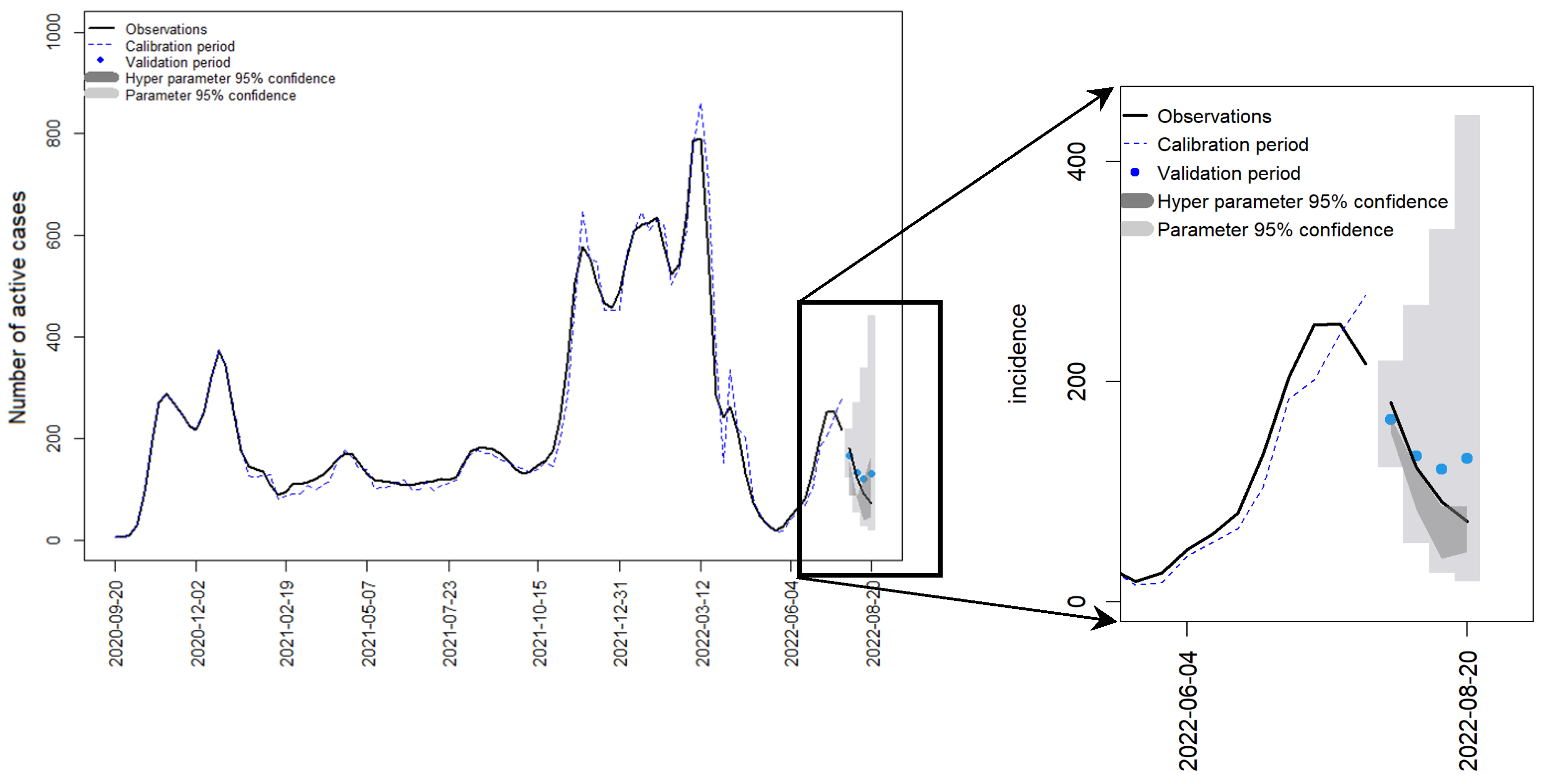
According to the conducted simulation sets, the Akaike information criterion (AIC) was computed. The AIC metric indicates the sweet spot model complexity by balancing the number of model parameters with the available empirical data. The AIC metric worsens as the models become more complicated (i.e., has more parameters). It should be noted that the model with the minimum AIC is not necessarily the optimum model structure, especially in terms of model complexity. Hence, among the best five percentile AIC equivalent model structures, the structure with the least complexity was selected as the best model. Applied to the current setting, the optimal model structure was SARIMA(0,2,1; 2,1,2), named as model No. 232 (all model structures are listed in the Supplementary Material), according to the metrics described. Figure 5 shows the prediction results for the calibration period, based on the best model structure for the epidemiology data of the Liechtenstein wastewater data.
As seen in Figure 5, the model predictions in the 4-week validation period matched the observation visually with moderate accuracy. For the selected structure, the correlation was calculated as 0.30, the RMSE as 97.82, and the RMSPE as 87%.
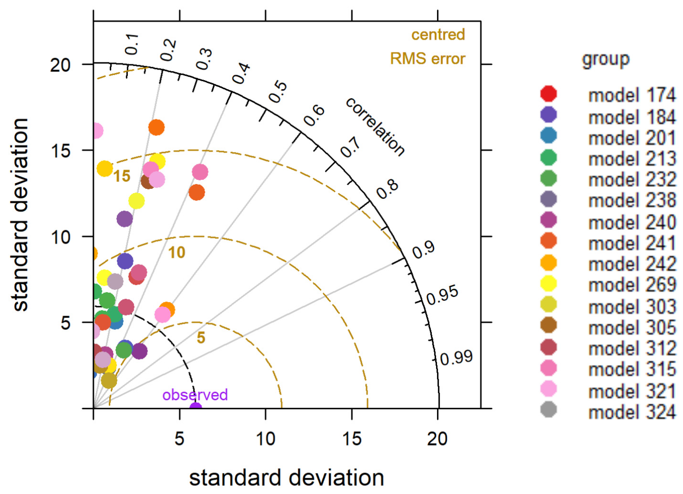
In spite of the successful implementation of SARIMA for the calibration period, it is beneficial to examine the diagnostic metrics for the validation data horizon as well. For selecting the best model structure with respect to the validation period, we checked the fitness of our models with the observations within the validation period. The RMSE and correlation for a selection of good model structures (above 95th percentile) were plotted through a Taylor diagram, shown in Figure 6. The standard deviation of the residuals between model prediction and ground truth is shown in radial distance. The azimuth angle displays correlation between predicted and ground truth. The RMS error is shown by the distance from the centered observation in purple.
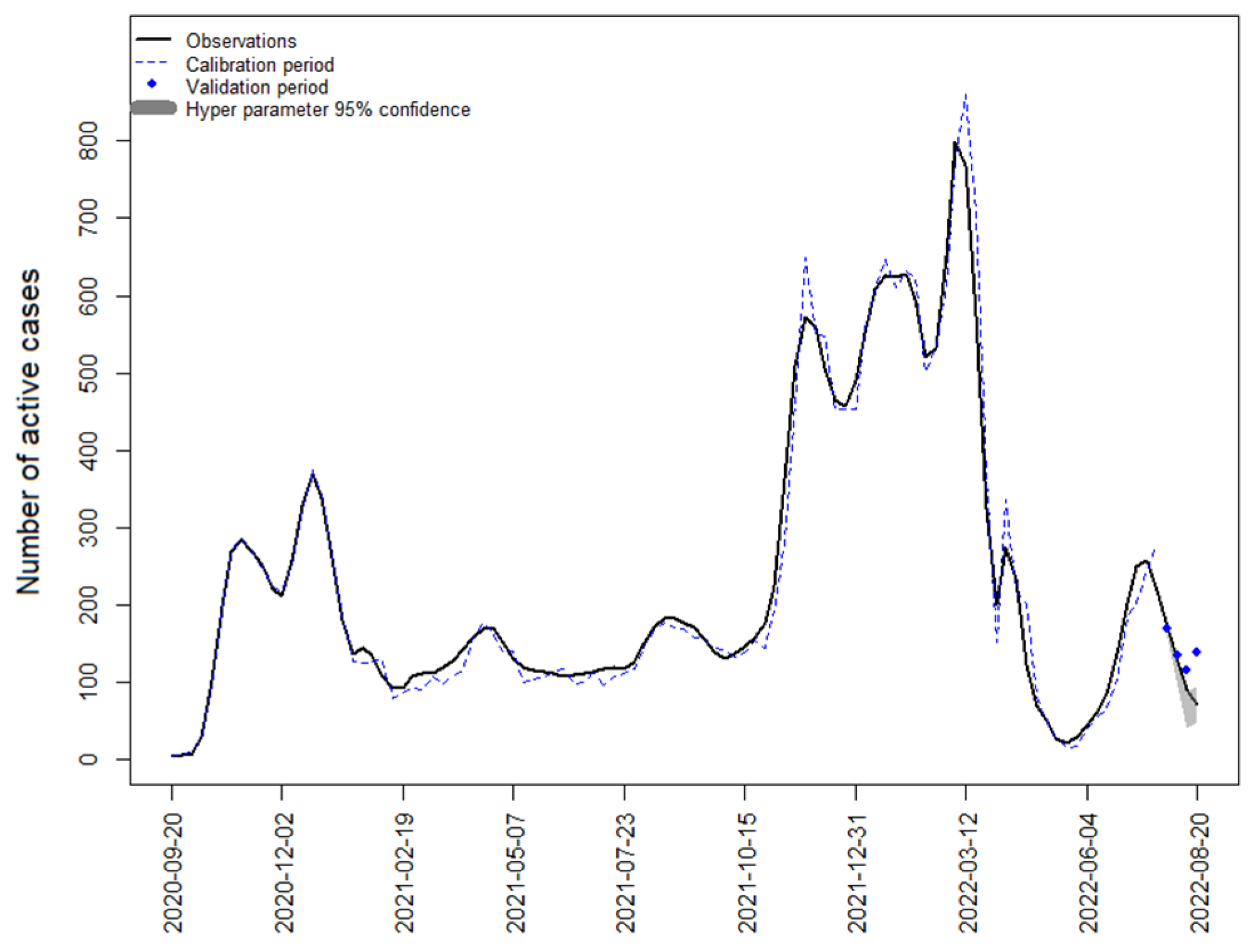
Figure 7 shows model predictions in the training and validation period; however, the best model structure was selected on account of the validation period. The RMSE and correlation for the employed model structure was calculated as 71.31 and 0.44, respectively (the RMSPE was calculated as 66%).

4.2. Strategy 2: SARIMAX Model with WBE Data

As outlined in the methodology section, this portion of this study employed the SARIMAX model class to explore and identify optimal model structures, incorporating the exogenous variable wastewater data. Similar to the procedure in the first strategy, the SARIMAX model was applied to the validation set. Model No. 238 was selected as the best model structure—which was SARIMAX (0,1,2; 2,1,2), according to the performance metrics. The selected model structure led to results with an RMSE of 100.03, an RMSPE of 95%, and a correlation of 0.54.
According to Figure 8, the model fitness was almost at the same level as compared to the univariate model without the wastewater data as an exogenous variable. The best model structures, employing the univariate strategy, resulted in RMSEs of 97.82 and 71.31, and correlations of 0.30 and 0.44 (depending on checking the calibration or the validation horizon). However, it is shown that by adding the WBE data as the exogenous variable, although the RMSE did not improve, the correlation between the results and the observations increased (the correlation for the best model structure with the WBE data was 0.54).

4.3. Strategy 3: SARIMAX Model with Mobility Data

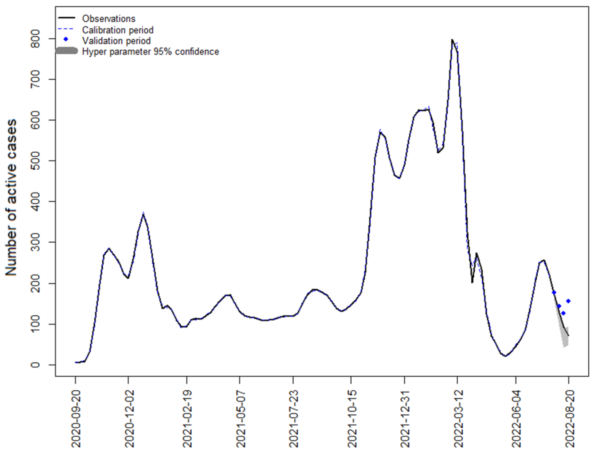
After evaluating the effect of wastewater data on COVID-19 prediction, the effect of the Google mobility data on total COVID-19 active cases was analyzed. Initially, the optimum model structure was obtained based on the validation set. Similar to the second strategy, model No. 323 showed the optimum results—SARIMAX (1,2,2; 2,2,2). The RMSE and correlation for this structure were 33.08 (the RMSPE was 91%) and 0.46, respectively. The model predictions were plotted during both the calibration and validation horizons, as depicted in Figure 9.
As seen in Figure 9, the fitness further improved, especially within the calibration horizon, as compared to other strategies, i.e., the univariate model (first strategy) and the multivariate model with WBE data (second strategy). This can mainly be attributed to the increase in model parameters, allowing it to better fit the data. The correlation stayed at similar levels, and the RMSE decreased considerably to 33 (the RMSE for other model strategies was between 70 and 100). In fact, the optimum model structure with mobility data had the best performance. This emphasizes the impact of social distancing and mobility restrictions during the course of the pandemic. However, the capability of WBE data in predicting the disease active cases should not be undervalued. In order to elaborate two main factors of mobility data—i.e., transit and workplace—and to further analyze and compare the effect of WBE data on the performance of the model structures, a sensitivity analysis was carried out.

4.4. Sensitivity Analysis of WBE and Mobility Data

A sensitivity analysis of the model performance influenced by the exogenous variables is displayed in this section. Additionally, the aim was to measure the uncertainty of each model prediction with respect to the model structures. The experiments were performed in the same way as in the previous strategies. However, the number of experiments was conducted equal to the number of exogenous variables. In other words, within a given trial, the model was evaluated across all plausible structures under the absence of one specific exogenous variable. This procedure was repeated for all the variables.
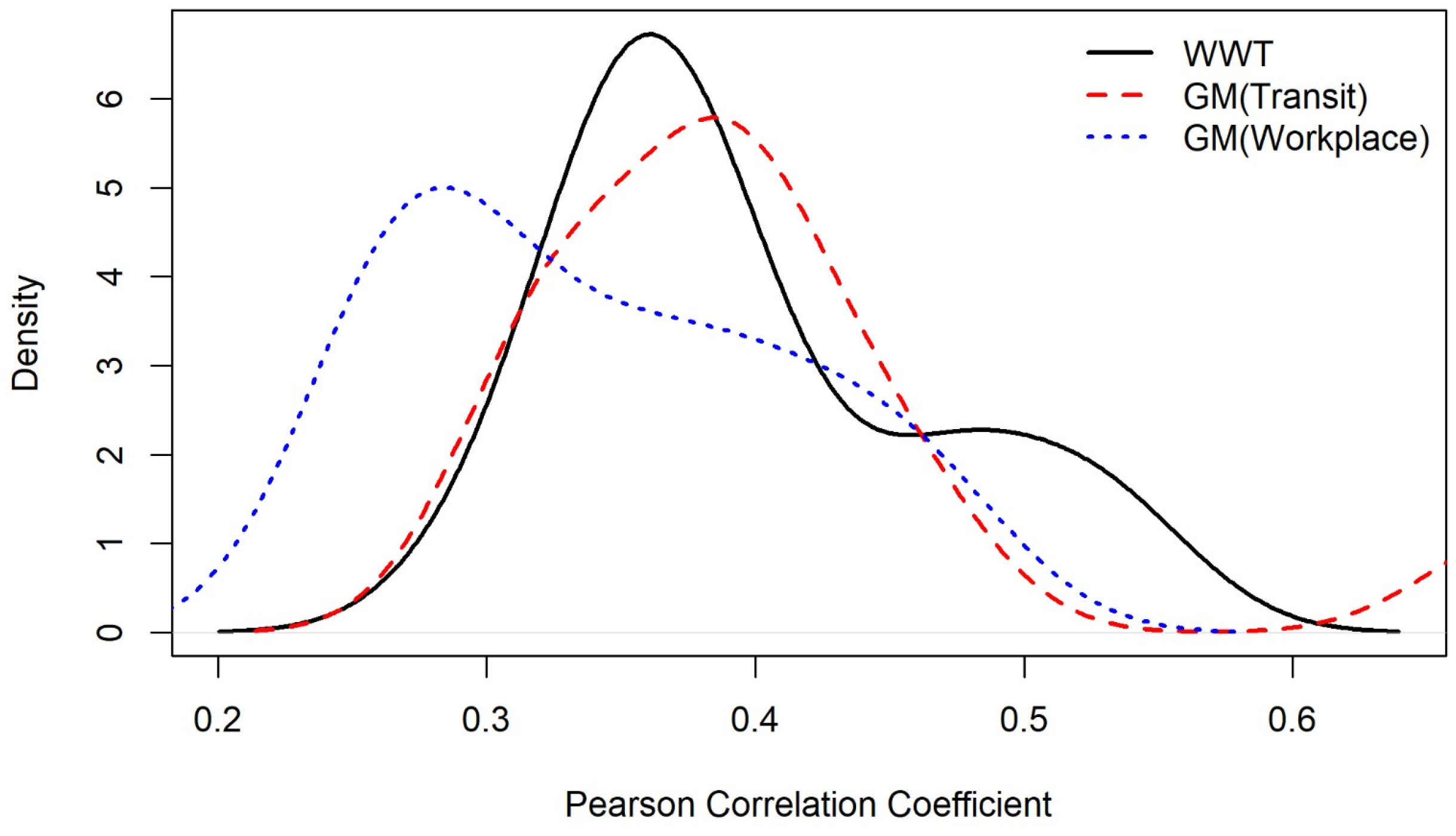
This part of this study includes three sets of exogenous variables: WBE data, Google mobility data in the transit sector, and Google mobility data in the workplace. Firstly, the WBE data were omitted from the calculations, and all the model structures (possible parameters of p, q, d, P, Q, and D) were tested on the validation set and evaluated with Pearson correlation. Similarly, this procedure was carried out for the mobility data in transit sector and workplace. The result is summarized and visualized as smoothed histograms of each strategy in Figure 10.
Figure 10 depicts the dependency of the model performance on each exogenous variable. In order to interpret this, the main factor to be considered was the mode (peak) of each density plot. It was seen that the peak of the workplace mobility lay below 0.3 correlation, which is the minimum amount, compared to the mobility data in transit and WBE data. This means that omitting the variable of mobility in the workplace had a high impact on the model performance. For model structures omitting WWT, the correlation increased moderately at around 0.5, which denotes that the model structure parameters possessed a high level of uncertainty. The uncertainty of model parameters was observable in all scenarios, when the WBE data or the mobility data in transit were omitted. The peaks of the two scenarios without WBE data and mobility data in transit stayed between 0.3 and 0.4. However, for the scenario without mobility data in transit, the peak lay closer to 0.4. This implies that the role of WBE data and mobility data in transit sector was similar in prediction efficiency.

4.5. Austrian Data

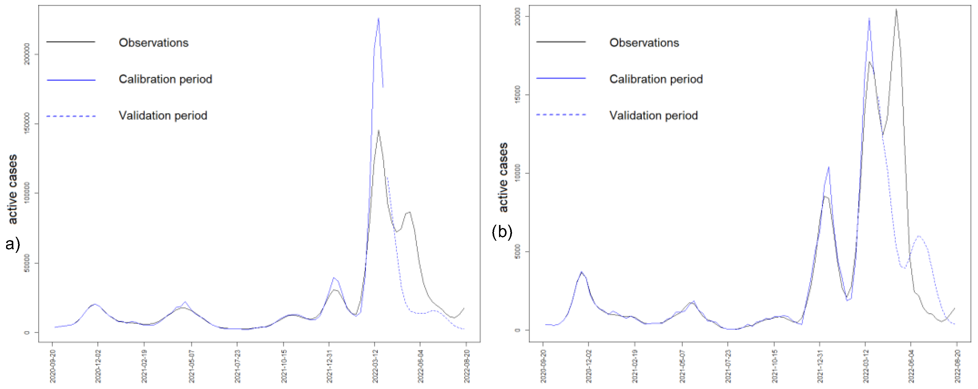
In order to further analyze the capability of the second strategy—using only WBE data as an exogenous variable—for predicting COVID-19 cases, we applied the WBE data of two federal states of Austria to the active cases as the main variable in Vienna and Vorarlberg, in a longer prediction horizon. To check the model’s prediction performance over a longer period, the prediction horizon was increased to twenty weeks. Indeed, the first 80% of the observations were dedicated to the calibration period, and the last 20% were categorized as the validation period. Afterward, the fitness of all the possible model structures against the observations was examined. The results are summarized in Figure 11. Figure 11a illustrates the model fitness performance in Vienna, and Figure 11b shows the model fitness for the validation horizons in Vorarlberg.
Figure 11 shows the model prediction and ground truth data in both Vienna and Vorarlberg. This exemplifies that the strategy of using a multivariate model with WBE data as an exogenous time series variable is capable of predicting the circulation of the SARS-CoV-2 virus in time periods longer than four weeks, although with less precision. However, the fitness of the optimum model result was lower, as compared to that for four-week time periods. With respect to the Vienna data, the optimum SARIMAX model structure was model No. 136 SARIMAX(0,0,0; 2,1,1). The RMSE and correlation for this structure were 32 and 0.66, respectively. As described before, the increase in RMSE was due to the higher case magnitude in the observed data in Vienna, compared to Liechtenstein. Thus, we need to consider the RMSPE, which was 56% in the case of Vienna. It can be seen that the employed strategy with WBE data produced satisfying results in predicting over long-term periods.

5. Conclusions

As forecasting the infection incidence of COVID-19 has a significant influence on restriction policies, finding the best strategy for the accurate prediction of active cases is necessary. Additionally, examining the correlation between restriction policies and active COVID-19 cases is crucial. The current study conducted several time series analyses to identify the optimal model structure for predicting disease prevalence. Our findings were as follows:
  • The optimal model fitness for predicting the number of COVID-19 cases was reached by employing SARIMAX models with either WBE or Google mobility data as exogenous factors, forecasting up to four weeks.
  • Transit mobility data and WBE data demonstrated similar capabilities in predicting active cases.
  • When the WBE data and mobility data were integrated into forecast models, they served as supplementary information to aid decision makers taking significant and appropriate restriction policies. The forecast accuracy was a function of finetuning the model parameters and the choice of exogenous variables.
Further exploration of the fundamental factors contributing to case prevalence and an investigation into other restriction policies, such as stay-at-home measures, workplace closures, event cancelations, and testing policies, is a prospect of future research.

Supplementary Materials

The following supporting information can be downloaded at https://www.mdpi.com/article/10.3390/environments11050100/s1: Figure S1: different policies and restriction levels deployed in Liechtenstein; Figure S2: the correlation diagram between the restriction policies and COVID active cases. Shape and colour of the circles outline the sign and strength of the correlation; Figure S3: the histogram (a) and QQ-plot (b) of Liechtenstein active cases time series, before BoxCox transformation; Figure S4: the histogram (a) and QQ-plot (b) of Vienna active cases time series, before BoxCox transformation; Figure S5: the histogram (a) and QQ-plot (b) of Vorarlberg active cases time series, before BoxCox transformation; Figure S6: the histogram (a) and QQ-plot (b) of Vienna active cases time series, after BoxCox transformation; Figure S7: the histogram (a) and QQ-plot (b) of Vorarlberg active cases time series, after BoxCox transformation; Figure S8: the ACF (a) and PACF (b) plots for the time series of Vienna active cases; Figure S9: the ACF (a) and PACF (b) plots for the time series of Vorarlberg active cases; Table S1: List of model structures.

Author Contributions

W.R. contributed to the paper in the following aspects: conceptualization, writing—review and editing, project supervision, and administration. R.A. contributed to the paper in the following aspects: conceptualization, methodology, software, data curation, and visualization. S.D. contributed to the paper in the following aspects: writing—original draft preparation, validation, and data curation. H.S. contributed to the paper in the following aspects: writing—review and editing, data curation, and visualization. H.I. and N.K. contributed to the paper in the following aspects: funding acquisition and editing. F.N. and R.M. contributed to the paper in the following aspects: methodology and data acquisition. M.B.-M. contributed to the paper in the following aspects: funding acquisition and writing—review and editing. All authors have read and agreed to the published version of the manuscript.

Funding

This research received no external funding.

Data Availability Statement

Data will be made available on request.

Conflicts of Interest

The authors declare no conflicts of interest.

References

  1. Shimko, K.M.; Piatkowski, T.; Thomas, K.V.; Speers, N.; Brooker, L.; Tscharke, B.J.; O’brien, J.W. Performance- and image-enhancing drug use in the community: Use prevalence, user demographics and the potential role of wastewater-based epidemiology. J. Hazard. Mater. 2021, 419, 126340. [Google Scholar] [CrossRef] [PubMed]
  2. Olesen, S.W.; Imakaev, M.; Duvallet, C. Making waves: Defining the lead time of wastewater-based epidemiology for COVID-19. Water Res. 2021, 202, 117433. [Google Scholar] [CrossRef] [PubMed]
  3. Wölfel, R.; Corman, V.M.; Guggemos, W.; Seilmaier, M.; Zange, S.; Müller, M.A.; Niemeyer, D.; Jones, T.C.; Vollmar, P.; Rothe, C.; et al. Virological assessment of hospitalized patients with COVID-2019. Nature 2020, 581, 465–469. [Google Scholar] [CrossRef] [PubMed]
  4. Polo, D.; Quintela-Baluja, M.; Corbishley, A.; Jones, D.L.; Singer, A.C.; Graham, D.W.; Romalde, J.L. Making waves: Wastewater-based epidemiology for COVID-19—Approaches and challenges for surveillance and prediction. Water Res. 2020, 186, 116404. [Google Scholar] [CrossRef] [PubMed]
  5. Rauch, W.; Schenk, H.; Insam, H.; Markt, R.; Kreuzinger, N. Data modelling recipes for SARS-CoV-2 wastewater-based epidemiology. Environ. Res. 2022, 214 Pt 1, 113809. [Google Scholar] [CrossRef]
  6. Fenz, G.; Stix, H.; Vondra, K. Austrian tourism sector badly hit by COVID-19 pandemic. Monet. Policy Econ. 2021, 41–63. [Google Scholar]
  7. Kuitunen, I.; Artama, M.; Haapanen, M.; Renko, M. Rhinovirus spread in children during the COVID-19 pandemic despite social restrictions—A nationwide register study in Finland. J. Med Virol. 2021, 93, 6063–6067. [Google Scholar] [CrossRef] [PubMed]
  8. Aberi, P.; Arabzadeh, R.; Insam, H.; Markt, R.; Mayr, M.; Kreuzinger, N.; Rauch, W. Quest for Optimal Regression Models in SARS-CoV-2 Wastewater Based Epidemiology. Int. J. Environ. Res. Public Health 2021, 18, 10778. [Google Scholar] [CrossRef] [PubMed]
  9. Betancourt, W.Q.; Schmitz, B.W.; Innes, G.K.; Prasek, S.M.; Brown, K.M.P.; Stark, E.R.; Foster, A.R.; Sprissler, R.S.; Harris, D.T.; Sherchan, S.P.; et al. COVID-19 containment on a college campus via wastewater-based epidemiology, targeted clinical testing and an intervention. Sci. Total Environ. 2021, 779, 146408. [Google Scholar] [CrossRef]
  10. Kumar, M.; Jiang, G.; Thakur, A.K.; Chatterjee, S.; Bhattacharya, T.; Mohapatra, S.; Chaminda, T.; Tyagi, V.K.; Vithanage, M.; Bhattacharya, P.; et al. Lead time of early warning by wastewater surveillance for COVID-19: Geographical variations and impacting factors. Chem. Eng. J. 2022, 441, 135936. [Google Scholar] [CrossRef]
  11. Cao, Y.; Francis, R. On forecasting the community-level COVID-19 cases from the concentration of SARS-CoV-2 in wastewater. Sci. Total Environ. 2021, 786, 147451. [Google Scholar] [CrossRef] [PubMed]
  12. Schenk, H.; Heidinger, P.; Insam, H.; Kreuzinger, N.; Markt, R.; Nägele, F.; Oberacher, H.; Scheffknecht, C.; Steinlechner, M.; Vogl, G.; et al. Prediction of hospitalisations based on wastewater-based SARS-CoV-2 epidemiology. Sci. Total Environ. 2023, 873, 162149. [Google Scholar] [CrossRef]
  13. Vannoni, M.; McKee, M.; Semenza, J.C.; Bonell, C.; Stuckler, D. Using volunteered geographic information to assess mobility in the early phases of the COVID-19 pandemic: A cross-city time series analysis of 41 cities in 22 countries from March 2nd to 26th 2020. Glob. Health 2020, 16, 85. [Google Scholar] [CrossRef]
  14. Google, COVID-19 Community Mobility Reports. Available online: https://www.google.com/covid19/mobility/ (accessed on 15 January 2024).
  15. Ribeiro-Dantas, M.d.C.; Alves, G.; Gomes, R.B.; Bezerra, L.C.; Lima, L.; Silva, I. Dataset for country profile and mobility analysis in the assessment of COVID-19 pandemic. Data Brief 2020, 31, 105698. [Google Scholar] [CrossRef] [PubMed]
  16. Markt, R.; Endler, L.; Amman, F.; Schedl, A.; Penz, T.; Büchel-Marxer, M.; Grünbacher, D.; Mayr, M.; Peer, E.; Pedrazzini, M.; et al. Detection and abundance of SARS-CoV-2 in wastewater in Liechtenstein, and the estimation of prevalence and impact of the B.1.1.7 variant. J. Water Health 2021, 20, 114–125. [Google Scholar] [CrossRef]
  17. Land Tirol, Coronavirus COVID-19 Informationen. Available online: https://www.tirol.gv.at/gesundheit-vorsorge/infekt/coronavirus/ (accessed on 15 January 2024).
  18. Landesverwaltung Fürstentum Liechtenstein, Bevölkerung. Available online: https://www.statistikportal.li/de/themen/bevoelkerung (accessed on 16 January 2024).
  19. Statistics Austria, Independent Statistics for Evidence-Based Decision Making. Available online: https://www.statistik.at/en/statistics/population-and-society/population/population-stock/annual-average-population (accessed on 23 January 2024).
  20. Kneuer, M.; Wallaschek, S. Framing COVID-19: Public Leadership and Crisis Communication By Chancellor Angela Merkel During the Pandemic in 2020. Ger. Politics 2023, 32, 686–709. [Google Scholar] [CrossRef]
  21. Daleiden, B.; Niederstätter, H.; Steinlechner, M.; Wildt, S.; Kaiser, M.; Lass-Flörl, C.; Posch, W.; Fuchs, S.; Pfeifer, B.; Huber, A.; et al. Wastewater surveillance of SARS-CoV-2 in Austria: Development, implementation, and operation of the Tyrolean wastewater monitoring program. J. Water Health 2022, 20, 314–328. [Google Scholar] [CrossRef] [PubMed]
  22. Rasero, F.J.R.; Ruano, L.A.M.; Del Real, P.R.; Gómez, L.C.; Lorusso, N. Associations between SARS-CoV-2 RNA concentrations in wastewater and COVID-19 rates in days after sampling in small urban areas of Seville: A time series study. Sci. Total Environ. 2022, 806 Pt 1, 150573. [Google Scholar] [CrossRef]
  23. Cheshmehzangi, A.; Sedrez, M.; Ren, J.; Kong, D.; Shen, Y.; Bao, S.; Xu, J.; Su, Z.; Dawodu, A. The Effect of Mobility on the Spread of COVID-19 in Light of Regional Differences in the European Union. Sustainability 2021, 13, 5395. [Google Scholar] [CrossRef]
  24. Wellenius, G.A.; Vispute, S.; Espinosa, V.; Fabrikant, A.; Tsai, T.C.; Hennessy, J.; Dai, A.; Williams, B.; Gadepalli, K.; Boulanger, A.; et al. Impacts of social distancing policies on mobility and COVID-19 case growth in the US. Nat. Commun. 2021, 12, 3118. [Google Scholar] [CrossRef]
  25. Box, G.E.P. Time Series Analysis: Forecasting and Control, 5th ed.; Wiley: Hoboken, NJ, USA, 2015; Available online: https://ebookcentral.proquest.com/lib/kxp/detail.action?docID=2064681 (accessed on 23 January 2024).
  26. Wei, W.; Jiang, J.; Liang, H.; Gao, L.; Liang, B.; Huang, J.; Zang, N.; Liao, Y.; Yu, J.; Lai, J.; et al. Application of a Combined Model with Autoregressive Integrated Moving Average (ARIMA) and Generalized Regression Neural Network (GRNN) in Forecasting Hepatitis Incidence in Heng County, China. PLoS ONE 2016, 11, e0156768. [Google Scholar] [CrossRef] [PubMed]
  27. Fattah, J.; Ezzine, L.; Aman, Z.; El Moussami, H.; Lachhab, A. Forecasting of demand using ARIMA model. Int. J. Eng. Bus. Manag. 2018, 10, 1847979018808673. [Google Scholar] [CrossRef]
  28. Sah, S.; Surendiran, B.; Dhanalakshmi, R.; Yamin, M. Covid-19 cases prediction using SARIMAX Model by tuning hyperparameter through grid search cross-validation approach. Expert Syst. 2022, 40, e13086. [Google Scholar] [CrossRef] [PubMed]
  29. Hyndman, R.J.; Athanasopoulos, G. Forecasting: Principles and Practice. Available online: https://otexts.com/fpp2/ (accessed on 6 August 2020).
  30. Katrakazas, C.; Michelaraki, E.; Sekadakis, M.; Ziakopoulos, A.; Kontaxi, A.; Yannis, G. Identifying the impact of the COVID-19 pandemic on driving behavior using naturalistic driving data and time series forecasting. J. Saf. Res. 2021, 78, 189–202. [Google Scholar] [CrossRef] [PubMed]
  31. Khatun, N. Applications of Normality Test in Statistical Analysis. Open J. Stat. 2021, 11, 113–122. [Google Scholar] [CrossRef]
  32. Mishra, P.; Pandey, C.M.; Singh, U.; Gupta, A.; Sahu, C.; Keshri, A. Descriptive statistics and normality tests for statistical data. Ann. Card. Anaesth. 2019, 22, 67–72. [Google Scholar] [CrossRef]
  33. Cawood, P.; van Zyl, T. Feature-Weighted Stacking for Nonseasonal Time Series Forecasts: A Case Study of the COVID-19 Epidemic Curves: Arxiv. Available online: https://europepmc.org/article/PPR/PPR454047 (accessed on 17 January 2024).
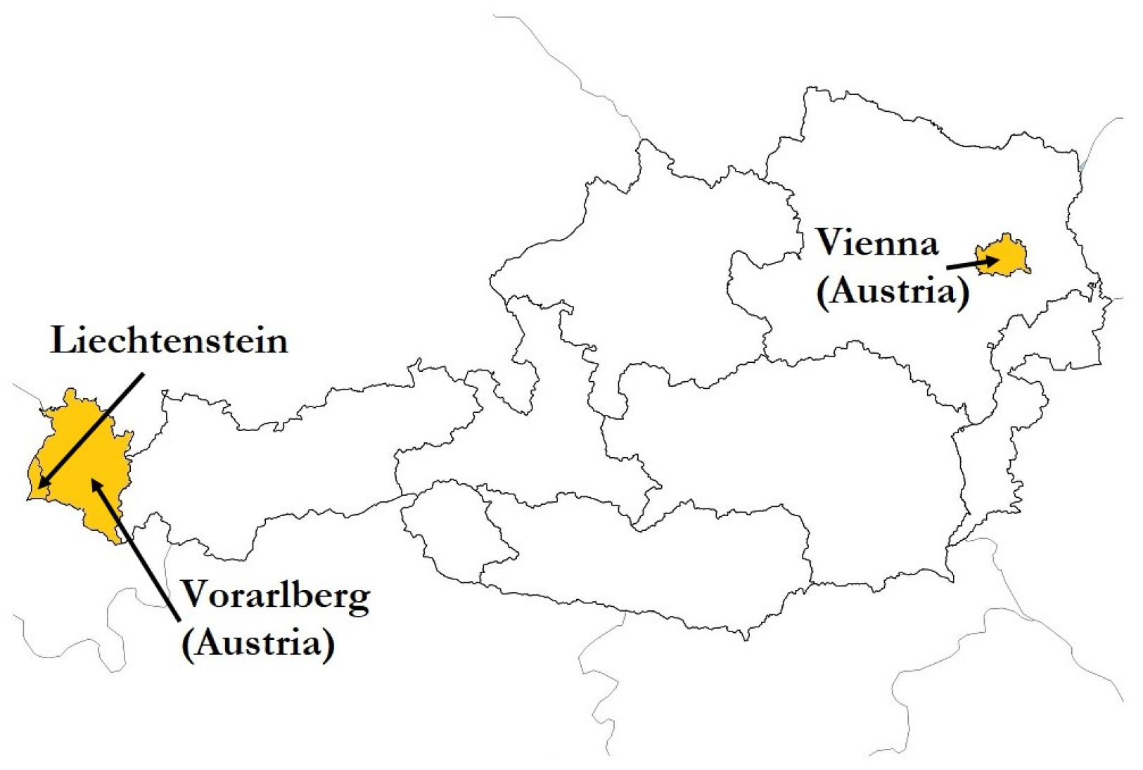
Figure 1. Location of Liechtenstein and two federal states of Austria: Vienna and Vorarlberg.
Environments 11 00100 g001
Figure 2. Histogram (a) and QQ-plot (b) of the Box-Cox-transformed WBE data in Liechtenstein.
Environments 11 00100 g002
Figure 3. ACF (a) and PACF (b) plots of the transformed Liechtenstein data.
Environments 11 00100 g003
Figure 4. Number of active cases (gray bars) and COVID-19 WBE data (red) in Liechtenstein.
Environments 11 00100 g004
Figure 5. Prediction of COVID-19 active cases in Liechtenstein based on best model structure including WBE data in the calibration period. Predictions over 4 weeks after were used for validation (gray confidence bars).
Environments 11 00100 g005
Figure 6. Taylor diagram of the prediction errors within the validation period.
Environments 11 00100 g006
Figure 7. Prediction of COVID-19 active cases in Liechtenstein based on the best model structure with WBE data in the validation period (gray confidence bars).
Environments 11 00100 g007
Figure 8. Prediction of COVID-19 active cases in Liechtenstein based on the best multivariate model structure with WBE data and clinical data within the validation period.
Environments 11 00100 g008
Figure 9. Prediction of COVID-19 active cases, based on the best multivariate model structure with clinical data and Google mobility data within the validation period.
Environments 11 00100 g009
Figure 10. Impact of exogenous variables (viral load in wastewater, transit mobility, and workplace mobility) on correlation with SARS-CoV-2 cases, depicted as density functions.
Environments 11 00100 g010
Figure 11. Prediction of COVID-19 active cases in Vienna (a) and Vorarlberg (b) based on the best multivariate model structure with clinical and WBE data within the validation period.
Environments 11 00100 g011
Table 1. Key figures of the studied regions.
Country RegionPopulationArea (km2)
Liechtenstein 39,055160
AustriaVienna1,923,825414
Vorarlberg400,4692601
Table 2. Forecasting strategies for COVID-19 active cases.
Strategy No.Model Response Variable Exogenous Variable
1SARIMAActive cases-
2SARIMAXWastewater data
3Google mobility data
4Sensitivity analysis *Wastewater and Google mobility data
* Sensitivity analysis is performed using SARIMAX by perturbing the input data.
Disclaimer/Publisher’s Note: The statements, opinions and data contained in all publications are solely those of the individual author(s) and contributor(s) and not of MDPI and/or the editor(s). MDPI and/or the editor(s) disclaim responsibility for any injury to people or property resulting from any ideas, methods, instructions or products referred to in the content.