Article

Simulating Agricultural Water Recycling Using the APEX Model

1
Digital Landscape Solutions LLC, Cheyenne, WY 82001, USA
2
Texas A&M AgriLife Research, Blackland Research Center, Temple, TX 76502, USA
*
Author to whom correspondence should be addressed.
Environments 2024, 11(11), 244; https://doi.org/10.3390/environments11110244
Submission received: 11 September 2024 / Revised: 21 October 2024 / Accepted: 26 October 2024 / Published: 6 November 2024
(This article belongs to the Special Issue Hydrological Modeling and Sustainable Water Resources Management)

Abstract

:
Irrigation plays a vital role in many agricultural crop production regions. Drainage water recycling (DWR) is a popular irrigation water management system that collects excess water drained from cropland fields and stores it in on-site reservoirs for reuse. The efficacy of these systems varies by location, climate, irrigation frequency, and crop demands. Simulating this system would be beneficial for assessing the impact of water and land management practices on agriculture and natural resources. This study presents the development of computational algorithms for DWR simulation with the Agricultural Policy Environmental eXtender (APEX) model, along with the results for 39 testing sites where both reservoir and drainage systems are adopted. Simulating a DWR system with the revised reservoir module, the APEX model simulates irrigation water reuse ranging between 29% and 93%; sediment reduction of around 66%; nitrogen loss reduction of 23% and 73% for the mineral and organic forms, respectively; and phosphorus loss reduction of 22% and 79% for the soluble and sediment-transported forms, respectively. In conclusion, the results provided by the APEX model for sediment loss reduction align with field data, but discrepancies for nitrogen and phosphorus losses emerged from this test.

1. Introduction

Irrigation plays a crucial role in agricultural crop production, accounting for 70–80% of water use in the world [1,2] and about 70% of global groundwater withdrawals [3]. Water demand from the agricultural sector is expected to increase in the future following the trend observed in the past two decades [2], with the largest agricultural water use in developing and low-income countries where the impact of climate change and increases in population and income will result in strong competition for water use [2]. Data from the Conservation Effects Assessment Project (CEAP) [4,5] reveal that irrigated cropland expanded to 49.7 million acres (about 201,000 km2) between 2013 and 2016, an 11% increase since the previous survey for 2003–2006 [6]. Agricultural irrigation water typically comes from groundwater storage or surface sources, including stormwater and recycled water. Small-scale reservoirs and ponds, often used for agricultural irrigation, are vulnerable to drought, making water management critical. To help conserve water and reduce groundwater use, the Natural Resources Conservation Service (NRCS) has implemented irrigation water management (IWM) programs. Examples include the tailwater recovery (TWR) system and the drainage water recycling (DWR) system. DWR systems capture and store surface and subsurface drainage water for supplemental irrigation during dry periods [7,8], distinguishing them from TWR systems, which only capture surface water [7,9]. By storing water on-site, DWR systems allow farmers to reuse it for crop irrigation when rainfall does not meet crop needs, reducing dependence on groundwater extraction.
DWR systems create a closed loop by capturing tile drainage water, storing it in an on-site reservoir, and reusing it for irrigation. This process not only conserves water but also improves surface and groundwater quality. Drainage water often carries nitrates and phosphorus, which are removed from the soil via percolation. Moursi et al. [10] found that implementing a DWR reduced total nitrogen (TN) and total phosphorus (TP) in reservoir effluents by 47% and 46%, respectively. Additionally, crops benefit from the nutrients dissolved in recycled irrigation water [11]. As climate change brings more frequent and prolonged droughts and intense storms [12], it is increasingly important to store and recycle drainage water to offset water deficits during dry periods. Therefore, water storage and recycling strategies can help develop climate-resilient agriculture.
The simulation models used in CEAP are the Agricultural Policy Environmental Extender (APEX) and the Soil and Water Assessment Tool/Hydrologic Unit Model of the United States (SWAT/HUMUS). CEAP is a multi-agency project led by the USDA-NRCS to quantify the effects of conservation efforts adopted on cropland, grazing land, wetlands located in agricultural areas, and wildlife (fish and wildlife species) at the national and watershed levels. In CEAP, a combination of farmer surveys and modeling data is used to evaluate and recommend various natural resource conservation management strategies, including sustainable water management practices. The farmer surveys were designed to capture the state of conservation practice adoption in U.S. croplands and have involved thousands of farmers. The first farmer survey was conducted in 2003–2006 (CEAP I), and a second survey was conducted in 2013–2016 (CEAP II).
The APEX model [13,14] was developed by the USDA Agricultural Research Service (USDA-ARS) and Texas A&M AgriLife (part of Texas A&M University). The model has undergone continuous updates and improvements since its inception to simulate new processes and management activities [15]. Within CEAP, APEX assesses field-level conservation strategies by simulating daily farmland management activities, soil erosion, soil organic carbon, and nutrient and pesticide dynamics [6]. This model has been applied in various contexts, including simulating cropping systems and watersheds that incorporate reservoirs. For instance, the APEX model simulated runoff and sediment in the Shoal Creek watershed in central Texas [16,17]. In the Shoal Creek watershed, gully plugs (also known as check dams) were simulated as small reservoirs, and the model realistically simulated runoff and sediment yield with an R2 ranging from 0.6 to 0.8 and Nash–Sutcliffe efficiency (NSE) ranging between 0.58 and 0.77. Similarly, Sharifi et al. [18] used APEX’s reservoir feature to simulate wetland ecosystems on the eastern shore of Maryland. This enhanced APEX model included a biogeochemical module, which successfully estimated sediment yield and organic nitrogen and provided acceptable results for NH4, though the model’s performance on NO3 and PO4 transport was marginal. Despite these challenges, the study demonstrated APEX’s capacity to model nutrient cycling effectively. In China, Luo and Wang [19] used the APEX model to simulate a large watershed and assess the impact of management strategies on crop yield and soil erosion. After calibration, the model reliably reproduced crop yields (RRMSE ≥ 0.93, NSE ≥ 0.48) and predicted soil erosion rates comparable to those observed in sediment cores from two reservoirs. These studies confirm APEX’s reliability in simulating agroecosystems that include reservoirs.
Building on the original APEX reservoir component, this study develops a modeling framework for simulating a DWR system within the APEX model. While the current version of APEX, APEX1501, can simulate either a reservoir or a drainage system independently, it cannot simulate both simultaneously for a single field. This limitation restricts the ability to simulate interactions between these two water management practices and evaluate the benefits of DWR systems in irrigated croplands. To address this limitation, our study expands the current reservoir module and integrates it with APEX’s drainage and irrigation components. This will enable the simulation of agricultural water recycling practices and their benefits to water quantity and quality of agroecosystems. The specific objectives of this study include (1) creating a hydraulic connection between reservoirs and tile drainage systems; (2) improving water and sediment routing through the combined system; (3) incorporating alternative irrigation sources when the reservoir’s stored water is insufficient; and (4) enhancing nutrient transport simulations by updating the nitrate mass balance in the topsoil layer to include inputs from recycled irrigation water. This updated APEX was tested using data from 39 CEAP II simulation sites in the Lower Mississippi, Texas Gulf Coast (LMTG), and South Central (SC) production regions [6]. Of those, 30 sites included both TWR systems and tile drains. Ultimately, the enhanced APEX will help quantify water conservation and water quality benefits of DWR systems on various cropping systems in the continental United States through CEAP II assessments.

2. Materials and Methods

The central focus of this activity involved developing modeling algorithms to represent DWR systems and updating the APEX model’s source code to enable the reliable simulation of DWR systems, particularly if tile drainage is implemented in the same area.

2.1. Reservoir Component Update

In APEX, one subarea—the smallest simulation unit characterized by uniform soil, management, weather, and slope [13,20]—may have one reservoir at its outlet. Reservoirs are designed with principal and emergency spillways to accommodate various structures. The inflow is derived from the subarea plus all other contributing subareas, if any. The reservoir water balance is described below:
R e s V = R e s V 0 + Q i n + R F V i n I r r E S E P Q o u t
where ResV and ResV0 are the final and initial reservoir contents (m3 d−1), Qin is the inflow rate (m3 d−1), RFVin is the rainfall rate (m3 d−1) on the pool area, Irr is the irrigation rate from the irrigation reservoir (m3 d−1), E is the evaporation rate (m3 d−1), SEP is the seepage rate (m3 d−1), and Qout is the outflow rate (m3 d−1). The reservoir surface area is used to estimate RFVin, E, and SEP as
R e s A = b 1 × R e s V b 2
b 1 = R e s A E / R e s V E × W S A × 10 b 2
b 2 = log R e s A E log R e s A P / log R e s V E log R e s V P
R F V i n = 10 × R F V × R e s
E = 10 × C L E × P E T × R e s
S E P = 10 × d t × R e s H C × R e s
where ResA is the reservoir surface area (ha) at the beginning of the day, b1 and b2 are coefficients derived from inputs for principal and emergency spillway elevations, ResAE and ResAP are the reservoir surface areas at emergency and principal spillway elevations (ha), ResVE and ResVP are the reservoir volumes at emergency and principal spillway elevations (m3), WSA is the area occupied by the reservoir (ha), RFV is the rainfall rate (mm d−1), CLE is a lake evaporation coefficient (0.6), PET is the potential evapotranspiration (mm d−1), dt is the time interval (24 h), and ResHC is the hydraulic conductivity of the reservoir bottom (mm h−1). The outflow (Qout, mm) is controlled by the two spillways and is calculated as
Q o u t = R e s V R e s V E × W S A × 10 ;   R e s V > R e s V E × W S A × 10
Q o u t = R R × 24 ;   R e s V P × W S A × 10 < R e s V < R e s V E × W S A × 10
Q o u t = 0.0 ;   R e s V < R e s V P × W S A × 10
where RR is the flow rate through the principal spillway (m3 d−1). Sediment content is calculated each day using the mass balance equation:
R e s Y = R e s Y 0 + Y i n Y o u t D e p
D e p = R e s V × Y Y 0
where ResY and ResY0 are the final and initial reservoir sediment contents (Mg), Yin and Yout are the sediment inflow and outflow (Mg), Dep is sediment deposition (Mg), and [Y0] and [Y] are the reservoir sediment concentrations in Mg m−3 at the start and end of a day. Reservoir sediment outflow, Yout (Mg d−1), is computed with the equation
Y o u t = Y × Q o u t
Organic N and P are transported to the reservoir via sediment particles. The organic nutrient content is calculated each day using the equation
R e s O N = R e s O N 0 + Y i n O N Y o u t O N D e p O N
where ResON0 and ResON are the initial and final organic N contents in kg, YinON and YoutON are the organic N inflow and outflow rates in kg d−1, and DepON is the organic N deposition rate in kg d−1. The deposition rate is estimated with the equation
D e p O N = O N × D e p
where [ON] is the concentration of organic N in the sediment in kg Mg−1. The ratio of organic N content to sediment content determines [ON], and the organic N outflow rate is computed as
O N = R e s O N 0 + Y i n O N / R e s Y 0 + Y i n
Y o u t O N = O N × Y o u t
Similar calculations are performed on organic P. Soluble N and P are considered conservative, and the daily content is calculated with the mass balance equation:
R e s S N = R e s S N 0 + Q i n S N Q o u t S N
where ResSN0 and ResSN are the initial and final soluble N contents in kg and QinSN and QoutSN are the soluble N inflow and outflow rates in kg d−1. The outflow rate is the product of flow and concentration.
Q o u t S N = S N × Q o u t
where [SN] is the soluble N concentration in the reservoir in kg m−3, which is estimated assuming complete mixing.
S N = R e s S N + Q i n S N / R e s V
Regarding the reservoir module, the original code is modified by subtracting the irrigation volume from the water volume in the reservoir. The original code is also modified to simulate the simultaneous adoption of reservoir and tile drainage systems. In particular, the original version of the APEX model sets the horizontal water flow that goes into the drainage system to zero when a reservoir is simulated in the same simulation unit (subarea). This instruction has been removed from the revised model’s source code. Therefore, the amount of water removed by the drainage system is subtracted from the soil profile and assigned to the tile drainage flow (Equation (21))
S W i = S W 0 i S E P H f l o w Q R F
where SWi is the water content (m3) of soil layer i, SW0i is the water content (m3) of layer i on the previous day, Hflow is the horizontal water flow component (m3 d−1), and QRF is the quick return flow rate (m3 d−1), which is equal to the tile drainage flow if the drainage system is located in soil layer i. Then, the drainage flow is accounted for in the calculation of the water yield as follows:
W Y L D = Q + R S S F + Q R F + H f l o w + Q D R + C P V H
where WYLD is the water yield (m3 d−1), Q is the surface water runoff (m3 d−1), and RSSF is the return subsurface flow (m3 d−1), which is the flow of water from aquifer storage (groundwater) returning to the soil surface downstream at the point of infiltration. In APEX, RSSF goes to the subarea outlet. QRF is the lateral flow of water from the soil profile that returns to the channel (m3 d−1). In APEX, QRF returns to the subarea outlet. Hflow is the part of the lateral flow within the soil profile (m3 d−1). In APEX, Hflow flows horizontally to the downstream subarea soil. QDR is the tile drainage flow (m3 d−1). When a drainage system exists in the soil, this flow captures part of the lateral subsurface flow and moves it with a shorter drainage time. CPVH is the horizontal pipe flow (m3 d−1) or crack or pipe flow. It is the flow of water moving through cracks and “natural pipes” present in the soil profile. An example of a “natural pipe” is the holes created by roots (dead and alive), which can be important in simulating forested areas (Figure 1). Finally, the water yield is calculated considering the tile drainage flow; it is routed to the reservoir and used to update the reservoir water volume.

2.2. Irrigation Reservoir Update

This modification provides water from a reservoir for irrigation when needed. If the amount of water in the reservoir is insufficient to meet irrigation needs, the difference will be supplied by other water sources. The volume of irrigation water required for the day can be provided as input data, or the model can estimate it based on the settings used for the simulation. The irrigation water volume (Irr) can be estimated based on the plant water stress level, the plant-available water deficit, or the soil water tension in the top 200 mm of the soil [21]. Once the irrigation water volume is estimated, the amount of water that can be provided by the reservoir (m3) is calculated as
R e s I r r = m i n R e s V ,   I r r
After the irrigation event, the term ResV is updated to consider the amount of irrigation water drawn from the reservoir.
R e s V = R e s V R e s I r r
Along with the amount of water provided by the reservoir, this model update considers the amount of mineral N dissolved in the irrigation water that goes to the mineral N pool of the topsoil layer
S o i l S N 1 = S o i l S N 1,0 + I r r S N
where SoilSN1,0 and SoilSN1 are the initial and final mineral (soluble) N content of the first soil layer (kg ha−1) and IrrSN is the soluble N content of the irrigation water provided by the reservoir (kg). IrrSN is calculated as
I r r S N = R e s I r r × S N
ResIrr and [SN] are calculated as reported in Equations (20) and (23).
Figure 2 represents the main processes and their interactions in the model development illustrated in the previous section.
The modifications presented here differ from those in other special versions of the APEX model published in the past. For instance, the APEX-Paddy module added to the APEX model by Choi et al. [22] offered a detailed simulation of the effects of paddy management on rice growth, water balance, and water quality, enabling the ponding of the subarea, control of water discharge, and actual evapotranspiration that exceeds potential evapotranspiration under wet conditions. In another version of the APEX model, Sharifi et al. [18] improved the ability of the model to simulate biogeochemical cycling in wetlands using the approach adopted in the WetQual model [23]. While these versions of the APEX model improve some features, none overcome the limitation of simulating a reservoir and a drainage system in the same field. The APEX update presented here is similar to that of Moursi et al. [8] for the DRAINMOD model, where the authors simulated DWR systems by simulating interactions between a reservoir and a field irrigated by the reservoir or that drained into the reservoir.

2.3. Study Sites

As mentioned in the introduction, these upgrades to APEX were tested using data from 39 CEAP II simulation sites. Of these, 33 sites are located in the LMTG production region, covering the states of Arkansas, Louisiana, Mississippi, and Texas, and 6 sites are located in the SC region falling in the states of Arkansas, Missouri, and Texas (Figure 3). These sites have numerous soil types: 20 fall under soil hydrologic group D, 15 under group B, and 4 under group C. Definition of soil hydrologic groups and their characteristics can be found in the National Engineering Handbook by the USDA-NRCS [24]. Soil drainage classes [25] range from well drained to poorly drained. A tile drainage system is in place at all the sites with soil in the somewhat poorly drained and poorly drained classes (30 sites in total). Annual precipitation in the study areas ranges from 1140 mm to 1670 mm, with an average of about 1300 mm. The most common cropping system is a rice–soybean rotation, while corn and winter wheat are grown in a few locations.

2.4. Field Data Acquisition

As reported in the previous section, data from CEAP II were used in this activity. Field-level data were originally collected from a subset of the National Resources Inventory (NRI) sample points on cultivated cropland fields. For these points, farmer surveys enabled the collection of information on field characteristics, the adoption of conservation practices, crop rotation, mineral and organic fertilizer applications, pesticide applications, irrigation practices, and the timing and equipment used for all field operations over the previous three years. The data collected through the farmer surveys can enable field-level simulations with the APEX model. Within the entire set of NRI sample points used for CEAP II field-level simulations, we selected a subset of points where the presence of a reservoir, a drainage system, and the reuse of irrigation water were reported. Unfortunately, the only information recorded in the surveys that could be useful for model calibration is the crop yield. However, owing to confidentiality issues, this cannot be disclosed or used here [6]. No other information, such as observed runoff, soil erosion, or nutrient losses, was collected in surveys conducted for CEAP I and II. Therefore, model evaluation is based on the average county yield reported by the USDA-NASS [26] and soil erosion and nutrient loss values reported in the scientific literature.

2.5. Simulation Setting

The APEX model was used to simulate 45 years, with the first 15 years serving as a spin-up period that was excluded from the results evaluation. Each site was simulated by replicating farmer-reported crop management, tillage practices, and any conservation practices in place. When the reservoir was added to the site configuration, it was placed within the upstream subarea where the cash crop was simulated and the irrigation water could be used. The variables used to set up the reservoirs in APEX are listed in Table 1 and are set based on the literature and the model developer’s recommendations. Values can vary widely depending on the size and location of the reservoir and spillway system. For example, the size of a DWR on-farm storage reservoir varies based on factors such as
(1)
The volume of water entering and leaving the reservoir.
(2)
The time the water remains in the reservoir.
(3)
The depth of groundwater.
Table 1. Variables for APEX Setup of Irrigation Reservoirs.
VariableDescriptionValue
RSEEElevation at emergency spillway (m)4.5
RSAESurface area at emergency spillway elevation (ha)1.0
RSVERainfall equivalent depth (or volume) over the surface area at emergency spillway elevation (mm)150
RSEPElevation at principal spillway (m)4.0
RSAPSurface area at principal spillway elevation (ha)0.95
RSVPRainfall equivalent depth (or volume) over the surface area at principal spillway elevation (mm)140
RSV0Initial volume (mm)140
RSRRAverage principal spillway release rate in days20
RSYSInitial sediment concentration (ppm)300
RSYNNormal sediment concentration (ppm)300
RSHCBottom hydraulic conductivity (mm h−1)0.00001
RSDPTime required to return to normal sediment concentration after runoff event (days)20
RSBDBulk density of sediment in the reservoir (Mg m−3)1.2
A generalized setting is reported in Table 1. The setup follows the guidelines provided by USDA NRCS for small dams, including PL-566 dams [27]. These guidelines specify placing the emergency spillway 0.5 to 1.5 m above the principal spillway to ensure safe flood management [28]. The 0.5 m difference in Table 1 between the emergency spillway (4.5 m) and the principal spillway (4.0 m) provides flexibility to handle floodwaters before the emergency spillway activates. This design is typical for small- to medium-sized reservoirs, especially those used for agricultural water management. The surface area at spillway elevation depends on topography and reservoir design. As reservoirs approach emergency spillway elevation, surface area typically increases [29]. For PL-566 dams, surface areas at emergency spillway elevation generally range from 0.5 to 2 ha [29], while at the principal spillway, they are usually smaller, often less than 1 ha [30]. For a reservoir with a surface area (WSA) of 1 ha at the emergency spillway, the water volume (V) in cubic meters corresponding to a depth of 150 mm (depthmm) can be calculated as
V = W S A × 10,000 × d e p t h m m / 1000 = 1500
This volume can also be expressed as a rainfall equivalent depth (Rainmm) in millimeters:
R a i n m m = V × 1000   W S A × 10,000 = 150  
Historical weather data, along with the frequency and intensity of extreme events and the water needs of cultivated crops, should be considered to estimate RSEE and RSAE. Irrigation reservoirs typically have a minimum depth of 10 ft (3.05 m, [31]), and the volume at the emergency spillway for a PL566 dam is typically around 150 mm [21].
Three scenarios are considered here:
  • No Reservoir (Baseline): Each point is simulated without the reservoir.
  • No Irrigation Reservoir (noIrr-Res): The reservoir is included in the configuration, but the water in the reservoir is not used for irrigation.
  • Irrigation Reservoir (Irr-Res): Adopting an irrigation reservoir is simulated.
All the other settings available in the APEX model, including general model parameters, are kept constant between locations (no point-specific parametrization and calibration) and between the scenarios described above.

2.6. Model Calibration and Validation

The settings of the APEX model used in this exercise are the same as those used in CEAP II simulations after model testing, verification, and subsequent validation. As reported by Williams et al. [17], model testing is based on approximately 88,000 runs, where APEX is executed for each run to ensure the model does not fail when simulating unusual soil–weather–management configurations. A smaller database of nearly 18,000 runs is later used to assess the results of the APEX simulations. In this case, model outputs are compared against spatially referenced data. For instance, county yields reported by the USDA-NASS [26] are compared against simulated crop yields, and the NRI-USLE estimates and NRI wind erosion estimates are used to evaluate simulated soil erosion rates. Simulated nutrient losses are compared against data included in the MANAGE database [32]. Following this scheme, the APEX model is calibrated for the entire set of runs available. During the validation process, simulated data from selected points are compared against experimental or observed data recorded under similar conditions to assess the model’s performance on various cropland ecosystems.

3. Results

3.1. Crop Yield

Before assessing the impact of reservoir adoption in the simulation sites, model performance was evaluated by comparing the simulated yield of the main crops grown at the selected locations against yields reported by the USDA-NASS [26]. As noted earlier, crop yield was the only datapoint collected at the field level through CEAP I and II farmer surveys. However, owing to confidentiality, the county yield data from USDA-NASS [26] were used for validation. No data on soil erosion or water quality were available for the CEAP II simulation points. The annual yield for 2013–2022 for each county where the simulation sites are located was used as the observed yield and compared against crop yield data for the last 30 years of simulation. After calibration, the APEX model produced average yields that closely matched those reported by the USDA-NASS [26] for the relevant counties (Figure 4). For all the crops, the average simulated yield fell within the standard deviation of the observed data, with rice showing the largest difference between the observed and simulated yields. The model’s good performance was further demonstrated by a low relative root mean squared error (RRMSE) of 7.29% (RRMSE ranges between 0% and 100% with lower values indicating better model performance) and a high R2 value of 0.98 (R2 ranges between 0 and 1, with 1 indicating a perfect fit between the observed and predicted values). Both the RRMSE and R2 were calculated with R (v4.4.1) [33] using the “Metrica” package [34]. According to the documentation for the Metrica package, the RRMSE and R2 can be calculated as follows:
R R M S E = 1 n P i O i 2 / O ¯
R 2 = S   P O 2 / S   P 2 S   O 2
where P indicates the predicted or simulated values, O is the observed values, Ō is the mean of the observed values, n is the number of observations, S2PO is the explained variance, and S2PS2O is the total variance.

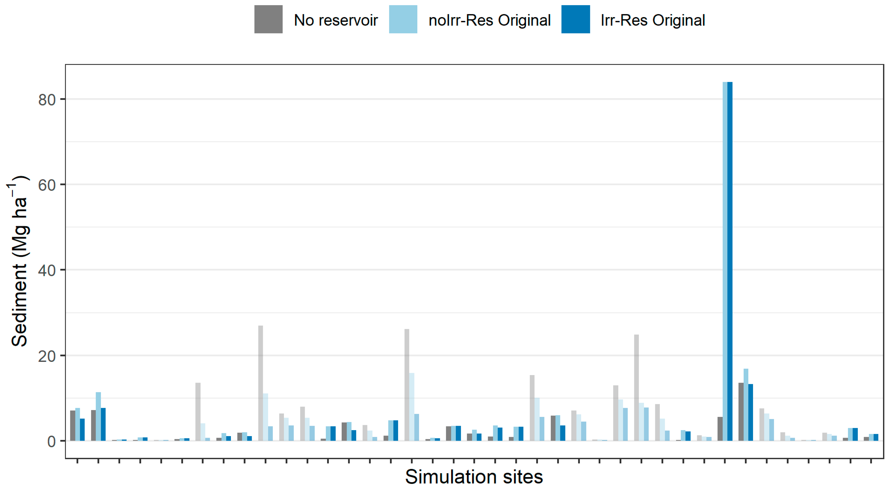
3.2. Sediment and Nutrient Losses with the Original APEX Model

In addition to evaluating crop yield, we also analyzed sediment and nutrient losses. Before enhancing the model, its outputs showed unrealistic and erroneous sediment and nutrient losses associated with the irrigation reservoir, particularly regarding sediment and TP losses. For example, at some CEAP II sites, the initial model results indicated increased sediment loss when a reservoir was included compared with the baseline scenario (Figure 5). This outcome was considered incorrect, as reservoirs typically function as sediment sinks by allowing particles to settle during water retention [35,36,37,38].
Unexpected results also emerged with TP losses when the reservoir was included in the simulation setting. Using opaque bars, Figure 6 highlights simulation sites where the model simulated higher P loss when the reservoir was included. This result was driven by the sediment simulation, as a large fraction of P (organic) is transported by sediment.
The unexpected results indicating higher sediment and P losses prompted a revision of the model to enhance its performance and reliability. The observed increase in sediment and P loss was due to a limitation in the original model code, which does not support the simultaneous simulation of a drainage system and a reservoir in the same subarea. Specifically, when a reservoir and a drainage system are simulated together, the original code sets the drainage system’s water to zero without removing it from the soil profile. This issue impacts the total soil water content and consequently affects runoff and soil erosion dynamics.
These unexpected results and an analysis of the model’s source code led to the APEX model’s revision, as detailed in Section 2. With the source code modification, the original APEX reservoir and drainage modules were retained, with only minor changes to connect them in order to simultaneously simulate a tile drainage system and reservoir, accounting for the water removed from the soil profile by the drainage system. One immediate consequence of the modification was a reduction in soil water content, resulting in a lower curve number, leading to lower runoff and soil erosion (the average values of the curve number were 80.1 and 73.5 with the original and revised source code, respectively). Following these adjustments, the APEX model produced more reasonable and expected results, as discussed in the subsequent sections.

3.3. Reused Water from Cropland

In this analysis, the impact of using irrigation water from a reservoir was compared with irrigation supplied solely from outside sources using the revised APEX model. The total annual irrigation amounts for the sites considered in this study ranged from 35 mm to 915 mm (averaging 370 and 380 mm yr1 for the supplemental only and reservoir + supplemental options, respectively). With the revised model, adopting a reservoir resulted in reusing 29% to 93% of the total irrigation water, corresponding to a minimum of about 24 mm to a maximum of 464 mm (average 190 mm) (Table 2 and Figure 7).
The results demonstrate that significant water savings can be achieved by storing excess irrigation water in a reservoir and reusing it throughout the season, reducing the demand for water from outside sources. Recycling water collected in the reservoir enables groundwater saving and the recycling of nutrients captured in the reservoir from the runoff of irrigation events, thus preventing nutrient loss to the downstream system [11]. This type of assessment was not feasible with the original version of the APEX model.

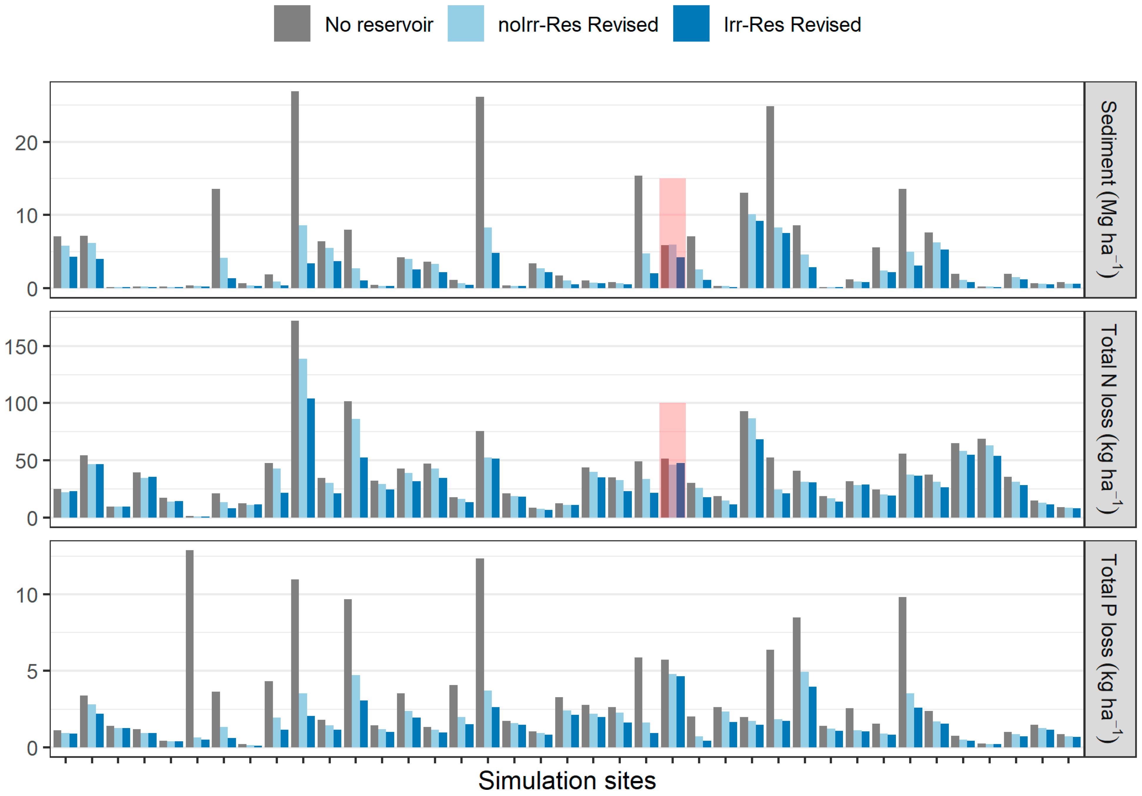
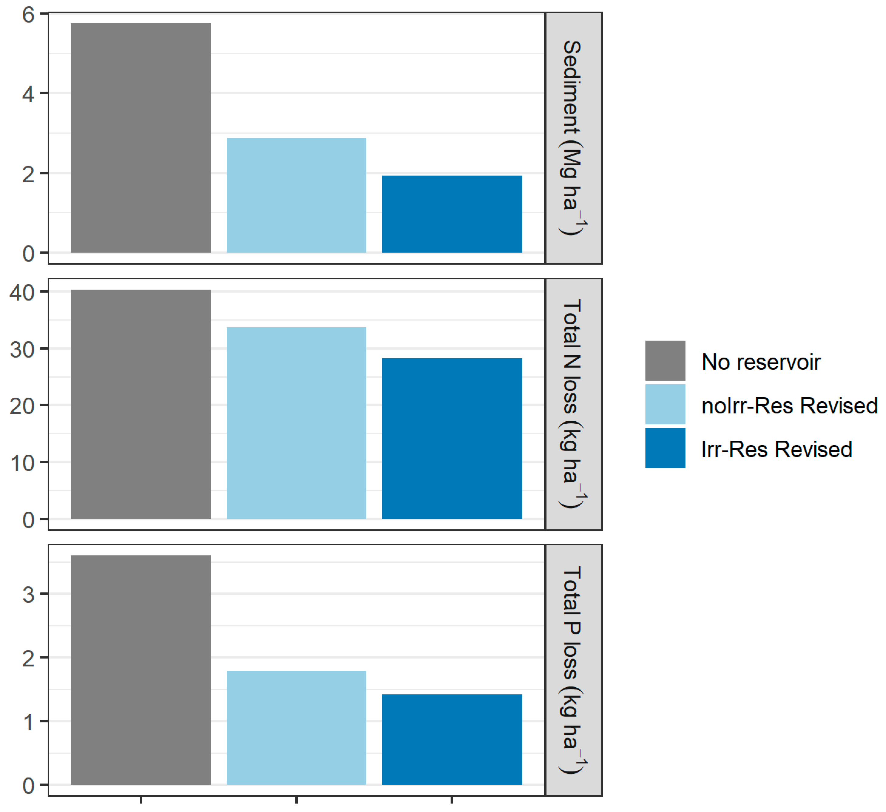
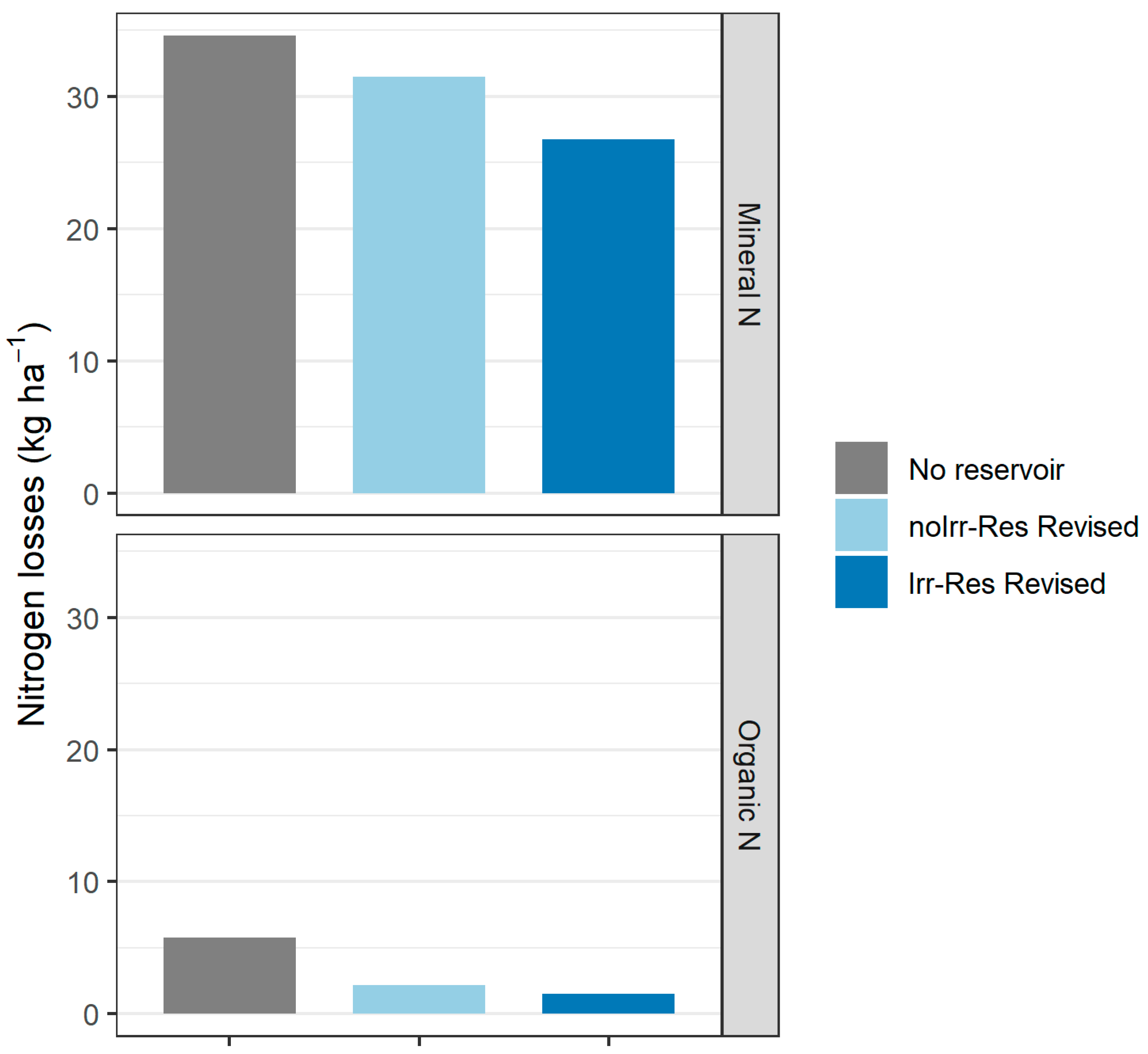
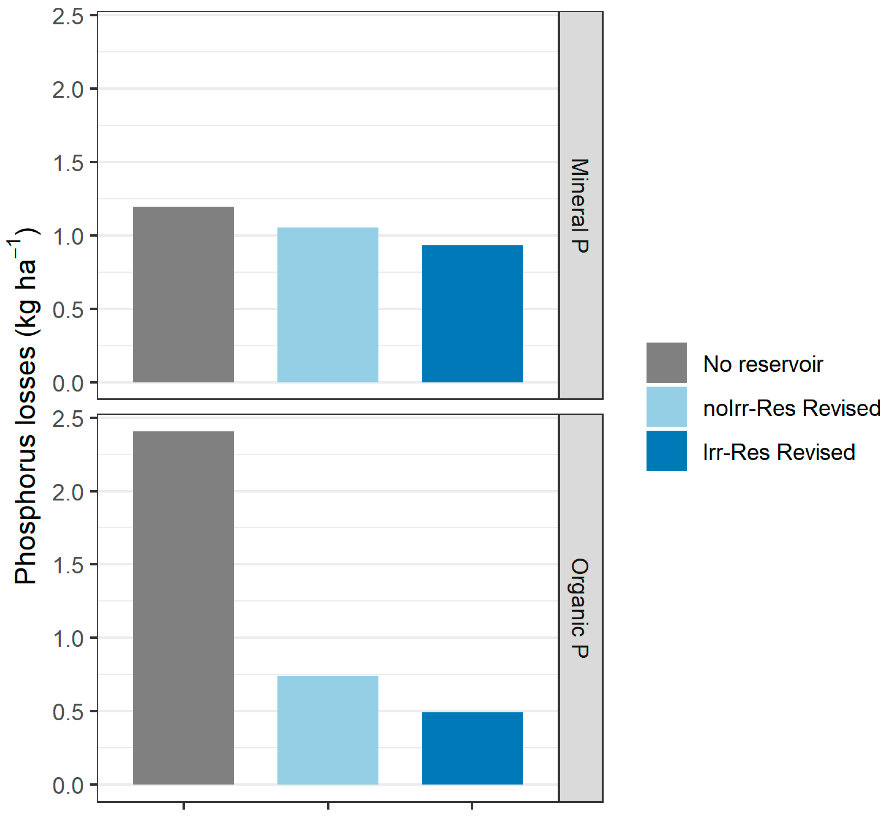
3.4. Sediment and Nutrient Losses

In the following section, we analyze the impact of adopting a reservoir on sediment, TN, and TP losses using the revised APEX model (Figure 8). The three scenarios described earlier are compared: No-Res (baseline), noIrr-Res, and Irr-Res.
Using the revised APEX model, reservoir adoption simulation reduced sediment, total N, and total P losses across all sites compared with the baseline scenario (Figure 8). The only exception was observed at one site (highlighted in red in Figure 8), where the revised model showed higher sediment losses in the noIrr-Res scenario and increased total N losses under the Irr-Res scenario. The higher sediment losses at this site can be attributed to a combination of significant precipitation and the fact that the reservoir water was not used for irrigation, leading to more significant overflow and subsequent soil erosion. For the total N losses, the general result confirms that the modifications introduced in the source code allowed us to obtain the expected results when simulating the adoption of a reservoir with or without a tile drainage system.
In analyzing the impact of adopting the reservoir on sediment and nutrient losses in the simulated sites, the model with the revised source code shows lower sediment yield for the noIrr-Res and Irr-Res scenarios, with 50% (−2.9 Mg ha−1) and 66% (−3.8 Mg ha−1) reductions, respectively, compared with the No-Res scenario. Similar results are produced for the total N and P losses. Simulated N losses are about 83% of the baseline for the noIrr-Res scenario and 70% for the Irr-Res scenario. The same trend can be observed for the P losses, with the revised model simulating a 1.8 kg P ha−1 reduction for the noIrr-Res scenario and a 2.2 kg P ha−1 reduction when the reservoir is used for irrigation (Figure 9).
To further analyze the impact of adopting a reservoir on N losses, the total losses are divided into mineral and organic fractions (Figure 10). Most nitrogen losses come from mineral N (86% to 95% of the total N losses, depending on the scenario), which is the soluble fraction that can be transported by water and is less affected by the implementation of the reservoir. Introducing a reservoir not for irrigation purposes can reduce the mineral N losses by about 9% (equal to about −3.1 kg N ha−1), and a limited 23% reduction (−7.8 kg N ha−1) is obtained by reusing irrigation water. A larger percentage reduction is simulated for the organic form of nitrogen (fraction attached and transported by sediment), with N losses reduction going from 62% (about 3.6 kg N ha−1 less) in the noIrr-Res scenario to 73% (about 4.2 kg N ha−1 reduction) in Irr-Res.
The revised model also simulates reductions in both mineral and organic phosphorus (P) losses (Figure 11). Unlike nitrogen losses, where the mineral fraction typically dominates, the most significant reduction in P losses varies depending on the scenario. When the reservoir is not included, the majority of P losses—about 67%—are in the organic form. When the reservoir is included in the simulation (the noIrr-Res and Irr-Res scenarios), the most significant fraction of P losses comes from mineral P, representing 59% and 65% of the total losses for the noIrr-Res and Irr-Res scenarios, respectively. This can be explained by the reservoir reducing sediment losses, which is how organic P is transported. Adopting the reservoir reduces the mineral P losses by 12% (0.1 kg P ha−1) and 22% (0.3 kg P ha−1) for the noIrr-Res and Irr-Res scenarios, respectively. A larger reduction is simulated for the organic fraction with −69% (−1.7 kg P ha−1) and −79% (−1.9 kg P ha−1) for the noIrr-Res and Irr-Res scenarios.

4. Discussion

Implementing DWR is a highly effective strategy for mitigating groundwater depletion, especially in regions where precipitation is insufficient or poorly timed to meet crop water needs. Additionally, DWR systems can significantly enhance water quality downstream of cultivated fields, particularly when paired with on-site storage reservoirs. This study revised the original reservoir component of the APEX model to simulate a DWR system coupled with a constructed on-farm storage reservoir. Given the increasing adoption of DWR systems, it is crucial for programs that evaluate the effects of human activities on the land, like CEAP, to assess the impact of such water management strategies on agroecosystems. The revised APEX model demonstrates that adopting a DWR system can lead to benefits consistent with findings in the scientific literature. In particular, compared with the baseline scenario (no reservoir), the revised APEX model shows reductions in sediment, nitrogen, and phosphorus losses when a reservoir is included, both with (Irr-Res) and without (noIrr-Res) water recycling for irrigation.
Directly calibrating the model for sediment and nutrient losses was not feasible owing to a lack of observed data for the CEAP II points used in this study. Instead, we assessed the model’s accuracy by comparing its outputs against field research observations. This comparison affirmed that the APEX model is a reliable tool for simulating a DWR system and its impact on the landscape. For example, Omer et al. [11] reported a 49% sediment reduction and 55% and 40% reductions in N and P losses, respectively. Similarly, Tan et al. [39] and Tan and Zhang [40] reported a 41% reduction in nitrate losses and a 12% reduction in total P losses after adopting a DWR system in Canada. Still in Canada, Drury et al. [41,42] reported a nitrate loss reduction of between 43% and 68% with a DWR system. More recently, Moursi et al. [10] reported the results of a field experiment designed to evaluate the effect of DWR on reducing sediment, N, and P losses. At the end of a two-year study, the authors reported an average reduction in sediment loss of 87%, while the N and P losses were reduced on average by 47% and 30%, respectively. These findings, especially those reported by Moursi et al. [10], are similar to the reductions in sediment, N, and P losses simulated with the revised APEX model. In our study, the revised APEX model predicted sediment loss reduction of between 50% and 66%. This range aligns with the values reported by the authors cited above. However, the model simulated a 17–30% reduction in the N losses and 50–60% in the P losses compared with the baseline scenario. These reductions are slightly outside the range of reductions reported in field research, indicating a probable underestimation of the N loss reduction and an overestimation of the P loss reduction due to adopting the DWR system.
The agreement between the model simulations and field data for sediment losses suggests that the modifications introduced to the code are effective and produce reliable results. However, the discrepancies observed in the simulations for N and P losses indicate that further calibration is needed. Extending model testing to include additional sites with a DWR system and collecting comprehensive data on water quantity and quality would be useful in enhancing the model’s accuracy. This approach would enable a more precise representation of field and watershed dynamics and improve the model’s ability to predict the effects of DWR systems on water and nutrient management.
The lack of specific data on water quantity and quality at sites with adopted DWR systems has limited the ability to calibrate the APEX model for these sites and reduce uncertainty. Nevertheless, the reliability of APEX’s reservoir module provides a solid foundation for assessing the benefits of DWR systems to sediment and nutrient reduction in discharge water. Given the increasing adoption of such systems in U.S. croplands, it is crucial to expand model testing with new sites and data on water quantity and quality. Moreover, further model enhancements may be required to simulate the potential reintroduction of sediment transported back to the cultivated and irrigated fields through irrigation water obtained from the reservoir.

5. Conclusions

This study presents significant advancements in simulating drainage water recycling (DWR) systems within the APEX model by integrating the tile drainage and reservoir components to evaluate the impacts on water quantity and quality. A closed loop was created by creating a hydraulic connection between the original reservoirs and drainage module and updating the water, sediment, and nutrient transport pathways, offering a robust framework for assessing DWR systems. Results from the revised model for selected CEAP II sites participating in irrigation water management programs demonstrate the potential benefits of DWR in reducing sediment, nitrogen, and phosphorus losses—aligning closely with field research findings. The APEX model simulated a reduction in sediment losses ranging from 50% to 60%, consistent with values observed in empirical studies. However, while sediment loss simulations strongly agree with the field data, discrepancies in nitrogen and phosphorus loss estimates suggest further model calibration is needed. The model’s slight underestimation of nitrogen loss reductions and overestimation of phosphorus loss reductions highlight areas for improvement. Using additional testing sites with data on water quantity and quality is important for enhancing model accuracy, enabling a more precise representation of agroecosystem dynamics.

Author Contributions

Conceptualization, X.W. and J.J.; methodology, L.D., X.W. and J.J.; software, L.D., X.W. and J.J.; validation, L.D. and X.W.; formal analysis, L.D. and X.W.; investigation, L.D. and X.W.; writing—original draft preparation, L.D.; writing—review and editing, L.D., X.W. and J.J.; visualization, L.D. All authors have read and agreed to the published version of the manuscript.

Funding

This research was funded by the U.S. Department of Agriculture’s Conservation Effects Assessment Project (CEAP), a multi-agency effort led by the Natural Resources Conservation Service (NRCS) to quantify the effects of voluntary conservation and strengthen data-driven management decisions across the nation’s private lands. Grant Agreement No 68-7482-17-355 and NR213A750023C014. For additional information on CEAP, please refer to https://www.nrcs.usda.gov/ceap, accessed on 28 October 2024.

Data Availability Statement

The datasets presented in this article are not readily available because of confidentiality issues. Requests to access the datasets should be directed to USDA-NRCS CEAP modeling team leader.

Acknowledgments

The authors thank Jimmy R. Williams for his invaluable and unwavering support while incorporating the modifications presented here into the APEX model.

Conflicts of Interest

The authors declare no conflicts of interest. The funders had no role in the design of the study; in the collection, analyses, or interpretation of the data; in the writing of the manuscript; or in the decision to publish the results.

References

  1. Shiklomanov, I.A. World Water Resources: A New Appraisal and Assessment for the 21st Century: A Summary of the Monograph World Water Resources; UNESCO: Paris, France, 1998. [Google Scholar]
  2. FAO. The State of Food and Agriculture 2020. In The State of Food and Agriculture (SOFA), 1st ed.; FAO: Rome, Italy, 2020; ISBN 978-92-5-133441-6. [Google Scholar]
  3. United Nations. (Ed.) Groundwater: Making the Invisible Visible; The United Nations World Water Development Report 2022; UNESCO: Paris, France, 2022; ISBN 978-92-3-100507-7. [Google Scholar]
  4. Johnson, M.-V.V.; Norfleet, M.L.; Atwood, J.D.; Behrman, K.D.; Kiniry, J.R.; Arnold, J.G.; White, M.J.; Williams, J. The Conservation Effects Assessment Project (CEAP): A National Scale Natural Resources and Conservation Needs Assessment and Decision Support Tool. IOP Conf. Ser. Earth Environ. Sci. 2015, 25, 012012. [Google Scholar] [CrossRef]
  5. Durincik, L.F.; Bucks, D.; Dobrowolski, J.P.; Drewes, T.; Eckles, S.D.; Jolley, L.; Kellogg, R.L.; Lund, D.; Makuch, J.R.; O’Neill, M.P.; et al. The First Five Years of the Conservation Effects Assessment Project. J. Soil. Water Conserv. 2008, 63, 185A–197A. [Google Scholar] [CrossRef]
  6. USDA-NRCS Conservation Practices on Cultivated Cropland: A Comparison of CEAP I and CEAP II Survey Data and Modeling; Natural Resources Conservation Service, U.S. Department of Agriculture: Washington, DC, USA, 2022.
  7. Hay, C.H.; Reinhart, B.D.; Frankenberger, J.R.; Helmers, M.J.; Jia, X.; Nelson, K.A.; Youssef, M.A. Frontier: Drainage Water Recycling in the Humid Regions of the U.S.: Challenges and Opportunities. Trans. ASABE 2021, 64, 1095–1102. [Google Scholar] [CrossRef]
  8. Moursi, H.; Youssef, M.A.; Chescheir, G.M. Development and Application of DRAINMOD Model for Simulating Crop Yield and Water Conservation Benefits of Drainage Water Recycling. Agric. Water Manag. 2022, 266, 107592. [Google Scholar] [CrossRef]
  9. Prince Czarnecki, J.M.; Omer, A.R.; Dyer, J.L. Quantifying Capture and Use of Tailwater Recovery Systems. J. Irrig. Drain. Eng. 2017, 143, 05016010. [Google Scholar] [CrossRef]
  10. Moursi, H.; Youssef, M.A.; Poole, C.A.; Castro-Bolinaga, C.F.; Chescheir, G.M.; Richardson, R.J. Drainage Water Recycling Reduced Nitrogen, Phosphorus, and Sediment Losses from a Drained Agricultural Field in Eastern North Carolina, U.S.A. Agric. Water Manag. 2023, 279, 108179. [Google Scholar] [CrossRef]
  11. Omer, A.R.; Moore, M.T.; Krutz, L.J.; Kröger, R.; Prince Czarnecki, J.M.; Baker, B.H.; Allen, P.J. Potential for Recycling of Suspended Solids and Nutrients by Irrigation of Tailwater from Tailwater Recovery Systems. Water Supply 2018, 18, 1396–1405. [Google Scholar] [CrossRef]
  12. Robinson, W.A. Climate Change and Extreme Weather: A Review Focusing on the Continental United States. J. Air Waste Manag. 2021, 71, 1186–1209. [Google Scholar] [CrossRef]
  13. Gassman, P.W.; Williams, J.R.; Wang, X.; Saleh, A.; Osei, E.; Hauck, L.M.; Izaurralde, R.C.; Flowers, J.D. The Agricultural Policy/Environmental eXtender (APEX) Model: An Emerging Tool for Landscape and Watershed Environmental Analyses. Trans. ASABE 2010, 53, 711–740. [Google Scholar] [CrossRef]
  14. Williams, J.R.; Izaurralde, R.C. The APEX Model. In Watershed Models; CRC Press: Boca Raton, FL, USA, 2010; pp. 437–482. [Google Scholar]
  15. Williams, J.R.; Arnold, J.G.; Kiniry, J.R.; Gassman, P.W.; Green, C.H. History of Model Development at Temple, Texas. Hydrol. Sci. J. 2008, 53, 948–960. [Google Scholar] [CrossRef]
  16. Wang, X.; Hoffman, D.W.; Wolfe, J.E.; Williams, J.R.; Fox, W.E. Modeling the Effectiveness of Conservation Practices at Shoal Creek Watershed, Texas, Using APEX. Trans. ASABE 2009, 52, 1181–1192. [Google Scholar] [CrossRef]
  17. Williams, J.R.; Potter, S.; Wang, X.; Atwood, J.; Norfleet, M.L.; Gerik, T.; Lemunyon, J.; King, A.; Steglich, E.M.; Wang, C.; et al. APEX Model Validation for CEAP. 2010; pp. 1–13. Available online: https://www.nrcs.usda.gov/sites/default/files/2023-04/ceap-crop-2010-APEX-Model-Validation.pdf (accessed on 1 July 2024).
  18. Sharifi, A.; Lee, S.; McCarty, G.; Lang, M.; Jeong, J.; Sadeghi, A.; Rabenhorst, M. Enhancement of Agricultural Policy/Environment eXtender (APEX) Model to Assess Effectiveness of WetlandWater Quality Functions. Water 2019, 11, 606. [Google Scholar] [CrossRef]
  19. Luo, Y.; Wang, H. Modeling the Impacts of Agricultural Management Strategies on Crop Yields and Sediment Yields Using APEX in Guizhou Plateau, Southwest China. Agric. Water Manag. 2019, 216, 325–338. [Google Scholar] [CrossRef]
  20. Wang, X.; Williams, J.R.; Gassman, P.W.; Baffaut, C.; Izaurralde, R.C.; Jeong, J.; Kiniry, J.R. EPIC and APEX: Model Use, Calibration, and Validation. Trans. ASABE 2012, 55, 1447–1462. [Google Scholar] [CrossRef]
  21. Steglich, E.M.; Osorio Leyton, J.M.; Doro, L.; Jeong, J.; Williams, J.R. Agricultural Policy/Environmental Extender Model User’s Manual—Version 1501; Blackland Research and Extension Center: Temple, TX, USA, 2019.
  22. Choi, S.-K.; Jeong, J.; Kim, M.-K. Simulating the Effects of Agricultural Management on Water Quality Dynamics in Rice Paddies for Sustainable Rice Production—Model Development and Validation. Water 2017, 9, 869. [Google Scholar] [CrossRef]
  23. Hantush, M.M.; Kalin, L.; Isik, S.; Yucekaya, A. Nutrient Dynamics in Flooded Wetlands. I: Model Development. J. Hydrol. Eng. 2013, 18, 1709–1723. [Google Scholar] [CrossRef]
  24. USDA-NRCS Hydrologic Soil Groups. In Part 630 Hydrology National Engineering Handbook; USDA-NRCS: Washington, DC, USA, 2007; Volume 210-VI-NEH.
  25. USDA-NRCS Chapter 2, Soils. In National Engineering Handbook. Irrigation Guide, Part 652; National Enginereeng Handbook; USDA-NRCS: Washington, DC, USA, 1997.
  26. USDA-NASS USDA—National Agricultural Statistics Service—Quick Stats Lite. Available online: https://www.nass.usda.gov/Quick_Stats/Lite/index.php (accessed on 15 October 2024).
  27. Woodward Donald, E. A Look Back at the Watershed Protection and Flood Prevention Act of 1954 (Pl-566). In Proceedings of the Watershed Management 2015, Reston, VA, USA, 5–7 August 2015; American Society of Civil Engineers: Reston, VA, USA, 2015; pp. 160–168. [Google Scholar]
  28. USDA-NRCS Articulated Concrete Block Armored Spillways. In National Engineering Handbook. NEH Part 628 Dams; USDA-NRCS: Washington, DC, USA, 2019.
  29. United States. Bureau of Reclamation Design of Small Dams; Water Resources Technical Publication; U.S. Department of the Interior, Bureau of Reclamation: Washington, DC, USA, 1987.
  30. Stephens, T. Manual on Small Earth Dams: A Guide to Siting, Design and Construction; FAO Irrigation and Drainage Paper; FAO: Rome, Italy, 2010; ISBN 978-92-5-106547-1. [Google Scholar]
  31. Sahoo, D.; Yazdi, M.N.; Owen, J.S., Jr.; White, S.A. The Basics of Irrigation Reservoirs for Agriculture; Clemson Cooperative Extension, Land-Grant Press by Clemson Extension: Clemson, SC, USA, 2021; LGP 1121. [Google Scholar]
  32. MANAGE Measured Annual Nutrient Loads from AGricultural Environments (MANAGE) Database. Available online: https://agdatacommons.nal.usda.gov/articles/dataset/Measured_Annual_Nutrient_loads_from_AGricultural_Environments_MANAGE_database/24660720 (accessed on 15 October 2024).
  33. R Core Team. R: A Language and Environment for Statistical Computing; R Foundation for Statistical Computing: Vienna, Austria, 2024. [Google Scholar]
  34. Correndo, A.A.; Rosso, L.H.M.; Hernandez, C.H.; Bastos, L.M.; Nieto, L.; Holzworth, D.; Ciampitti, I.A. Metrica: An R Package to Evaluate Predictionperformance of Regression and Classification Point-Forecastmodels. J. Open Source Softw. 2022, 7, 4655. [Google Scholar] [CrossRef]
  35. McDowell, R.W.; Biggs, B.J.F.; Sharpley, A.N.; Nguyen, L. Connecting Phosphorus Loss from Agricultural Landscapes to Surface Water Quality. Chem. Ecol. 2004, 20, 1–40. [Google Scholar] [CrossRef]
  36. Iseyemi, O.O.; Farris, J.L.; Moore, M.T.; Locke, M.A.; Choi, S. Phosphorus Dynamics in Agricultural Drainage Ditches: An Influence of Landscape Properties. J. Soil Water Conserv. 2018, 73, 558–566. [Google Scholar] [CrossRef]
  37. Iseyemi, O.; Reba, M.L.; Haas, L.; Leonard, E.; Farris, J. Water Quality Characteristics of Tailwater Recovery Systems Associated with Agriculture Production in the Mid-Southern US. Agric. Water Manag. 2021, 249, 106775. [Google Scholar] [CrossRef]
  38. Kondolf, G.M.; Gao, Y.; Annandale, G.W.; Morris, G.L.; Jiang, E.; Zhang, J.; Cao, Y.; Carling, P.; Fu, K.; Guo, Q.; et al. Sustainable Sediment Management in Reservoirs and Regulated Rivers: Experiences from Five Continents. Earths Future 2014, 2, 256–280. [Google Scholar] [CrossRef]
  39. Tan, C.S.; Zhang, T.Q.; Drury, C.F.; Reynolds, W.D.; Oloya, T.; Gaynor, J.D. Water Quality and Crop Production Improvement Using a Wetland-Reservoir and Draining/Subsurface Irrigation System. Can. Water Resour. J. 2007, 32, 129–136. [Google Scholar] [CrossRef]
  40. Tan, C.S.; Zhang, T.Q. Surface Runoff and Sub-Surface Drainage Phosphorus Losses under Regular Free Drainage and Controlled Drainage with Sub-Irrigation Systems in Southern Ontario. Can. J. Soil Sci. 2011, 91, 349–359. [Google Scholar] [CrossRef]
  41. Drury, C.F.; Tan, C.S.; Gaynor, J.D.; Oloya, T.O.; Welacky, T.W. Influence of Controlled Drainage-Subirrigation on Surface and Tile Drainage Nitrate Loss. J. Environ. Qual. 1996, 25, 317–324. [Google Scholar] [CrossRef]
  42. Drury, C.F.; Tan, C.S.; Reynolds, W.D.; Welacky, T.W.; Oloya, T.O.; Gaynor, J.D. Managing Tile Drainage, Subirrigation, and Nitrogen Fertilization to Enhance Crop Yields and Reduce Nitrate Loss. J. Environ. Qual. 2009, 38, 1193–1204. [Google Scholar] [CrossRef]
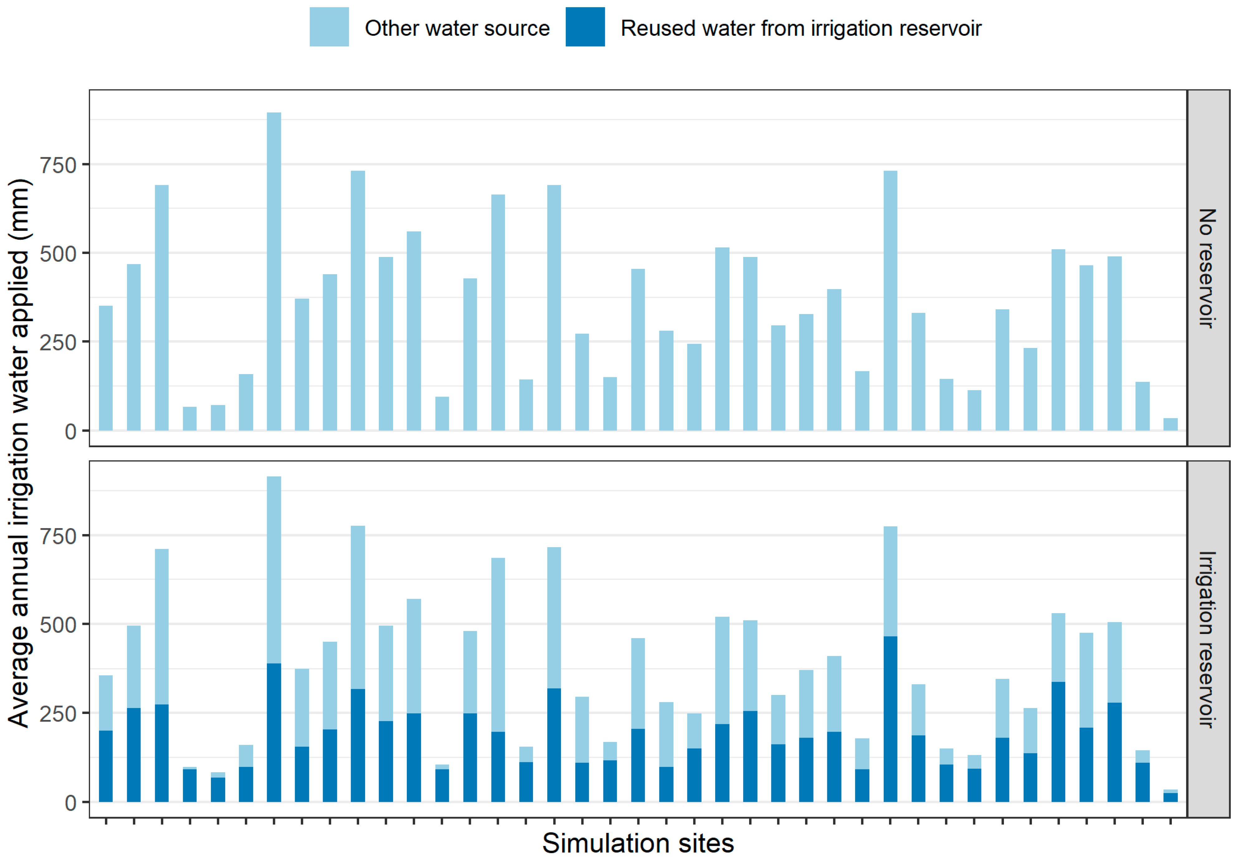
Figure 1. Graphical representation of the water flows in relation to soil and channel simulated by the APEX model.
Environments 11 00244 g001
Figure 2. Flowchart of the processes involved in the reservoir simulation.
Environments 11 00244 g002
Figure 3. Simulation sites (some points overlap each other).
Environments 11 00244 g003
Figure 4. Simulated and observed average crop yield (standard deviation reported in error bars).
Environments 11 00244 g004
Figure 5. Sediment loss with and without a reservoir in the model setting. Opaque bars indicate simulation sites where the original model produced unrealistic results.
Environments 11 00244 g005
Figure 6. Total phosphorus loss with and without a reservoir in the model setting. Opaque bars indicate simulation sites where the original model produced unrealistic results.
Environments 11 00244 g006
Figure 7. Average annual total irrigation and recycled water use.
Environments 11 00244 g007
Figure 8. Sediment (top), total nitrogen (middle), and total phosphorus (bottom) losses were simulated with the revised APEX model for the three scenarios. Highlighted in red is the only site where the revised model showed higher sediment losses in the noIrr-Res scenario and increased total N losses under the Irr-Res scenario.
Environments 11 00244 g008
Figure 9. Sediment (top), total N (middle), and total P (bottom) losses were simulated for the three scenarios with the revised APEX model.
Environments 11 00244 g009
Figure 10. Mineral (top) and organic (bottom) average N losses for the three scenarios.
Environments 11 00244 g010
Figure 11. Mineral (top) and organic (bottom) average P losses for the three scenarios.
Environments 11 00244 g011
Table 2. Total Irrigation Water and Breakdown Between Sources.
Supplemental Source OnlyReservoir + Supplemental Source
Total Irrigation
(mm yr−1)
Total Irrigation
(mm yr−1)
Reused Water from Percolation
(mm yr−1)
Irrigation from
Supplemental Source
(mm yr−1)
Minimum35.035.024.56.8
Maximum895.0915.0464.2526.3
Average370.0380.1189.8196.0
Disclaimer/Publisher’s Note: The statements, opinions and data contained in all publications are solely those of the individual author(s) and contributor(s) and not of MDPI and/or the editor(s). MDPI and/or the editor(s) disclaim responsibility for any injury to people or property resulting from any ideas, methods, instructions or products referred to in the content.

