Copper Speciation in Wine Growing-Drain Waters: Mobilization, Transport, and Environmental Diffusion

Abstract

Copper (Cu) has been used to treat vines for a long time, which has led to its accumulation in vineyard soils. In the present work, the mobilization of copper from these soils and its transport, and diffusion outside the plots by drain water were investigated. For this, the distribution of copper between the dissolved and colloidal phases, and within the colloidal phase, of these waters was determined using an investigation strategy based on the coupling between a size separation technique, asymmetric flow field-flow fractionation, and several detectors. First, the total copper concentrations in water from different drains were monitored over a period of 2 years: Cu was mainly found in the fraction of < 450 nm. Then, the distribution of copper on the size continuum was more closely studied in water from one of the drains, sampled over a winter period. Between 45 and 75% of Cu was found in the 2–450 nm colloidal fraction. The <450 nm colloidal phase of the drain waters was found to be mainly composed of humic acids (~15 to 60 mg L⁻¹) and clay-rich particles (~100 to 650 mg (Al) L⁻¹). These particles also contained (hydr)oxides of iron and manganese. The concentrations of Fe and Mn were approximately 100 to 200 times lower than those of Al. The majority of humic acids had an apparent molar mass of ≤ 10 kDa. They were distributed along the size continuum: (i) in a population with an average size of ~20 nm, probably consisting of supramolecular entities, and (ii) associated with clay-rich particles with a size of ~120–200 nm. Copper was found to be complexed with humic acids and associated with clays via clay-humic complexes. Copper mobilization from the soil to the water and its transport to the drain water appeared governed by the soil humidity level and the rainfall.

1. Introduction

The speciation of a chemical element is recognized as essential knowledge to understand the role and fate of this element in a given environment. Trace element speciation is therefore determined and used in environmental sciences and all related fields [1]. However, although the term speciation is widely used, it does not always have the same meaning, depending on the scientific field involved. Beforehand, it is therefore useful to agree on its meaning. Thus, speciation in a multiphasic medium as soil is defined as the distribution between the different forms in which an element could exist [2]. Note that the notion of “forms” is not specified, which enables this definition to remain open. This is especially relevant when different parts of an ecosystem are considered, e.g., water and soil or sediments, the atmosphere, and living organisms.

Depending on the scientific question, it may be useful to do the following: (i) characterize, more or less finely, the phases (solid, dissolved, or gaseous) in which the element is found and the components with which the element is associated; (ii) determine the distribution of the element accordingly; and/or (iii) individually identify and quantify the different chemical species of this element. In all cases, it is essential to take into account the physical heterogeneity of an environment, the interfaces (notably solid-dissolved or ubiquitous in the environment) inherent to these heterogeneities, and the dissolved/colloidal size continuum governing the presence of the element in aqueous and porous environments and the atmosphere. Indeed, the complexed and/or particle forms of an element can have a size ranging from a few tens to a few hundred nanometers, therefore being located in this submicrometric continuum [1,3,4]. The influence of the size of these forms on the behavior and fate of the element is not taken into account without this size continuum. This can lead to missing part of the element and underestimating its role in an environment. However, the colloidal phase is recognized as playing a key role in the biogeochemical cycles of elements and chemical species [4,5,6,7]. It is in particular the place where processes of sorption/desorption, complexation/dissociation directly involving the element, and dissociation, dissolution, and agglomeration/aggregation of the carrier phases indirectly involving the element occur. All these processes directly concern the dissolved/colloidal size continuum and may even concern the particle phase beyond the micrometer, typically when large agglomerations/aggregations and subsequent settling/sedimentation occur. These phenomena can therefore lead to phase changes and modify the mobility, accessibility, and availability of elements [4].

To identify, characterize, and quantify an element in a size continuum, a multi-criteria (or multidimensional) analytical approach is needed in order to access the main characteristics describing the colloidal objects involving the element of interest. This requires using several detectors (multidetection). It also appears useful to base this approach on a separation method because this enables the sample to be simplified before the identification, characterization, and quantification of the analytes. Separation methods coupled online with detectors are therefore the most relevant to use [8,9,10]. They are also more respectful of the physical and chemical integrity of colloidal assemblies and much better resolved than the batch ultrafiltration methods [11]. Among these online size separation methods, Asymmetric Flow Field-Flow Fractionation (AF4) has a special place. Indeed, it is a gentle separation method with the absence of a stationary phase, enabling shear forces and interactions with the separation system to be limited. The separation system is thus both more robust and less impactful than a filled chromatographic column; the raw suspensions can be directly analyzed [12,13,14]. The separation power of AF4 is also important, typically 5 to 10 times more than chromatographic methods such as steric exclusion or hydrodynamic chromatography [8,15,16].

In order to monitor the evolution of the size according to the retention time without calibration, multi-angle light scattering (MALS) is a detector of choice in the submicrometer range. The signal measured by MALS depends on both the concentration of the analyte, its squared gyration size, and its molar mass [17]. The size of gyration, generally expressed as a radius or diameter with reference to a homogeneous hard sphere, depends on the physical size of the analyte and the mass distribution within it [18]. To monitor trace elements, inductively coupled plasma mass spectrometry (ICP-MS) is ideal due to its sensitivity and selectivity. To obtain additional chemical information, UltraViolet-Visible (UV-Vis) spectrometry proves relevant, particularly in environmental studies to monitor the chromophoric groups present in natural organic matter such as humic substances. In particular, UV-Vis spectrometry can be used as a concentration detector with defined and constant operating conditions [19]. A UV-Vis Diode Array Detector (DAD) is also interesting to use for speciation by accessing the spectrum, and therefore molecular information [18,20,21].

In this study, we use AF4-multidetection to determine the speciation (distribution) of Cu in the colloidal phase, which remains little studied compared to speciation in the dissolved phase. One of the environmental challenges identified is that of colloidal mobilization and transport. To illustrate the ways in which AF4-MALS-UV-Vis-ICP-MS can address this challenge, which is also linked to current environmental management issues, we chose to take copper in wine-growing areas as an example. Indeed, in order to fight against mildew, a pathogenic fungus of the vine, a fungicide based on inorganic copper salt (Bordeaux mixture, CuSO₄ + Ca(OH)₂) has been used for many years. This practice has led to an accumulation of copper in the upper part of the vineyard soils. Thus, different concentrations can be found, ranging from 30 mg (Cu) kg⁻¹ on average to well above 100 mg (Cu) kg⁻¹ [22,23,24]. Copper sulfate is a salt that dissociates easily. When vines are leached by rainwater, copper reaches the soil surface in a soluble Cu²⁺ form. According to the literature, copper can then be complexed with the organic and inorganic ligands of the solid phase of the soil (in order of affinity of the main ligands: clays, iron, and manganese oxides). Copper appears mainly chelated by soil organic matter (by its phenolic and carboxylic groups); these complexes are more stable than those with inorganic ligands. In soil water (i.e., suspension corresponding to the fraction below 0.45 µm), Cu is found either in the form of free ions or chelated to “dissolved” organic matter (DOM), complexed with inorganic ligands (e.g., hydroxyl, (hydrogeno) carbonate, sulfide, sulfate, etc.), or sorbed on sub-micrometric colloidal objects. Usually, copper speciation in soil water appears to be dominated by complexes with organic matter [25,26,27,28,29,30]. Although essential for living organisms, in too high concentrations in soils, copper can affect the activity of microorganisms and the growth of plants [22,23]. Another question also arises, that of the transport of copper from the surface of the soils where the vines are treated to (sub)surface water and ultimately river water. Such environmental spreading presents a significant risk to aquatic organisms due to the biocidal properties of copper [31]. This question is related to that of the mobilization from the solid phases of the soil to the water. A better understanding of this mobilization process means being able to anticipate it and better manage it, and ultimately a better control of the environmental diffusion of copper.

2. Materials and Methods

2.1. Site and Samples

Water and soil samples were obtained from a Sauternes vineyard located about 40 km from the city of Bordeaux and were previously studied [32]. A drainage network for the vineyard plots is present at a depth of approximately 0.6 to 0.8 m. On this vineyard, the Bordeaux mixture has been used for at least 80 years; the vines are treated between April and September. The water samples were all collected at the exit of their drain. During a preliminary monitoring phase, drain water was sampled in several vineyard plots every six months over a period of 2 years, and always outside the period of treatment with the Bordeaux mixture. Based on the preliminary phase, and for the speciation investigation, three water samples were collected from one specific drain, during a period of 4 months that had an average rainfall greater than the rest of the year (December, February, and April before the first treatment, i.e., in a period distant from the last treatment with the Bordeaux mixture). The average characteristics of the samples were a pH of 5.3 ± 0.1 (range of values: 0.2 pH unity) and a conductivity of 232 ± 5 µS cm⁻¹ (range of values: 78 µS cm⁻¹). The main colloidal components observed were: clays, mineral salts (from silt), other crystalline particles, and humic acids (HA). In parallel, the soils of the plots corresponding to the drains monitored were sampled vertically to the drain route. Plots of soils of the same nature and texture, i.e., soils with a sandy matrix that were more or less gravelly and hydromorphic, were considered. Their average characteristics consisted of the following: a pH between 5 and 6; approximately 1% organic matter, mainly humic acids; between 15% and 18% clays; around 9% fine silt and 7% coarse silt; 15% fine sand and more than 50% coarse sand; and a total copper concentration of around 65 mg kg⁻¹ with approximately 3 mg kg⁻¹ of exchangeable copper (extraction with 1 mol L⁻¹ of ammonium acetate at a pH of 7). The aim of this soil sampling was not only to determine the total and exchangeable copper but also to prepare leachates under conditions simulating rainfall, in order to carry out additional characterizations [33].

2.2. Chemicals

Ammonium nitrate (NH₄NO₃; Sigma-Aldrich, Steinheim, Germany) was used with 18.2 MΩ cm⁻¹ of ultrapure water (Milli-Q grade; Millipore, Bedford, MA, USA) to prepare the mobile phase of asymmetric flow field-flow fractionation (10⁻⁵ mol L⁻¹ of NH₄NO₃ at a pH of 6 for drain waters and soil leachates). They were filtered at 0.1 µm with Durapore filters (Millipore) before use. Solutions of sodium hydrogen carbonate and potassium hydrogen phthalate were used to calibrate the Total Organic Carbon analyzer (TOC) (Nacalai Tesque, Kyoto, Japan), for the inorganic carbon measurements and the total carbon measurements respectively.

2.3. Instruments and Operating Conditions

A centrifugal ultrafiltration (CUF) PierceTM Protein Concentrator (Thermo Scientific) with a 10 kDa regenerated cellulose membrane was used for the following: (i) to prepare colloidal test samples taken as laboratory reference materials for evaluating the analytical method performances; and (ii) to determine the apparent molar mass of the organic matter (OM). The centrifugal ultrafiltration method was applied with a concentration factor of 10, corresponding to the low threshold of the concentration range usually used, and with a liquid/solid ratio (L/S) of 10 [11,34]. In these conditions, the recovery was found to be 90 ± 10%.

A rotary shaker (Intelli-Mixer RM-1, Latvia) was used to prepare leachates as follows: 10 g of dried and sieved (2 mm stainless steel sieve) soil samples were mixed with 100 mL of ultrapure water; the mixture was stirred at 20 rpm for 24 h then decanted for 48 h at 4 °C away from light; finally, the supernatant was collected and filtered at 0.45 μm [11,33].

An Eclipse 3 AF4 instrument (Wyatt Technology, Dernbach, Germany) was used with a channel 26.5 cm long, and 2.1 (inlet) to 0.6 (outlet) wide. A spacer 250 µm thick was used to analyze the drain water samples and a 350 µm thick spacer for the leachate samples. A 10 kDa regenerated cellulose membrane (operational cut-off threshold determined experimentally at approximately 2 to 3 nm) was used for both types of samples. An Agilent Technologies 1100 series isocratic pump equipped with a micro vacuum degasser was used to deliver the flows (injection, focus, elution, cross-flow). The fractionation operating conditions were as follows: injection at 0.2 mL min⁻¹ with a focus flow rate of 3 mL min⁻¹ for 6 min (during which the dissolved phase was removed via the cross-flow and the colloidal phase was concentrated at the head of the channel); and fractionation with a channel flow rate of 0.6 mL min⁻¹ and a cross-flow rate of 0.45 mL min⁻¹ for 50 min. The AF4 recovery was determined with laboratory reference materials (procedure described elsewhere [35,36]); it was found to be 90 ± 10% to 100 ± 10% depending on the samples considered. The AF4 was coupled with the following:

• A UV-Vis spectrophotometer (Agilent Technologies 1100 series from Agilent, VWD G1314A, Tokyo, Japan) with a wavelength set at 254 nm to monitor organic matter. Beforehand, the proportionality of the response of the organic carbon to its concentration in the water suspensions considered was verified as described by Harguindeguy et al. [33]. Indeed, a constant molar extinction coefficient at the selected wavelength is a prerequisite for using UV-Vis as a concentration detector [19]. A UV-Vis DAD (1260 Infinity series, Agilent Technology, Tokyo, Japan) was used to provide organic matter spectra. The spectra were recorded between 200 and 700 nm, on samples filtered at 0.45 µm and fractionated by AF4;
• A multi-angle light scattering (MALS) detector (DAWN HELEOS, Wyatt Technology, Santa Barbara, CA, USA) to determine the gyration diameters online. The UV-Vis and MALS data were collected and processed with Astra 5.3.4.18 software (Wyatt Technology). The gyration radii and diameters were calculated using Zimm’s first-order fitting formalism;
• An atomic mass spectrometer (ICP-MS) (Agilent 7500ce; Agilent Technology, Tokyo, Japan) equipped with a Meinhard nebulizer, a refrigerated Scott chamber (2 °C), and a collision reaction cell (CRC) used in hydrogen mode. The AF4-ICP-MS coupling was carried out by a two-pump assembly (as precisely described elsewhere [37]). This assembly enabled both the fractionated colloidal particles to be carried to the ICP-MS, and the element standards to be introduced into the ICP-MS. According to the elemental composition previously determined in the considered samples (see Section 2.1 above), the monitored trace and major elements were ⁶³Cu, ⁶⁵Cu, ²⁷Al, ⁵⁴Fe, ⁵⁶Fe, ³⁹K, ⁵⁵Mn, ²³Na, ⁶⁴Zn, and ⁶⁶Zn.

The elemental concentrations and their distribution in waters and leachates were determined as follows: For monitoring: the samples were previously filtered at 0.45 µm then directly introduced into the ICP-MS to determine the total elemental concentration in the dissolved-colloidal (<0.45 µm) continuum. Additionally, the filters were mineralized (under a microwave field by a mixture of HNO₃/HF/H₂O₂, 6/2/2 mL) to determine the elemental concentration in the >0.45 µm compartment. For speciation: samples were introduced into the ICP-MS via the AF4 injection system. The AF4 system was operated as follows: (a) injection and elution to determine total elemental concentration over the dissolved-colloidal continuum; (b) injection, focus, and elution to determine the elemental colloidal concentration in the colloidal phase (i.e., >2–3 nm corresponding to the AF4 membrane cut off [34]). In steps (a) and (b), either the entire colloidal phase (approximately up to 1000 nm) was considered in the raw (unfiltered) sample, or only the colloidal phase up to approximately 450 nm was considered by filtering the sample beforehand. Concentrations in the dissolved phase were deduced from (a) and (b). For step (c), injection, focus, fractionation, and elution were used to determine the elemental colloidal distribution in the colloidal phase (only carried out on filtered samples). Each analysis was at least duplicated. The accuracy of the elemental determination was previously verified by the analysis of laboratory reference solutions (for ICP-MS analysis) and laboratory reference suspensions (for AF4-ICP-MS analysis) [37].

2.4. Signal and Data Processing

2.4.1. Signal Filtering

A digital low-pass filter was used to filter the signals of the fractograms recorded by the detectors (MALS, UV-Vis, and ICP-MS). The processing considers noise as a random signal added to the useful signal. To attenuate the noise, a part (denoted a) of the filtered signal was mixed with the raw signal (i.e., the signal before filtering). The quantity “a” corresponds to the filtering coefficient. In the resulting mixture, the signal is amplified by (1 + a) and it shifts by an increment “b” depending on the filter coefficient. It is therefore necessary to de-amplify the signal and to readjust its increment. The corresponding equation is as follows:

S_f(t_i) = [S(t_i+b) + a S_f(t_i−1+b)] × [1 + a]⁻¹

(1)

In this equation, S_f is the filtered signal, S is the raw signal, i is the increment corresponding to the ith recorded value of the signal at the time t_i (i taken between 2 and n, the number of recorded values of signal S(t_i)), a is the filter coefficient, and b the shift correction coefficient. S_f(t₁) is taken equal to S(t₁). Usually, according to the noise intensity and the number n, 0 < a ≤ 30. In the present case, a = 7 to 10, and b = a − 2, for n = 4000 approximately.

2.4.2. UV-Vis Spectral Characterization

In the colloidal phase (which is typically the case when spectra are recorded during AF4 fractionation), the intensity of the transmitted light, and therefore the absorbance, depends not only on the absorption of the light emitted by the chromophoric groups of chemical species (Lambert-Beer law) but also on the light scattered by analytes in suspension, i.e., colloidal objects. The light scattering (see Section 2.4.5 below) depends on the geometry of the detector, the number of colloidal objects, and, when the diameter of these analytes is >0.05 λ, their squared gyration radius. Thus, when a UV-Vis spectrum is recorded between approximately 200 and 750 nm, light scattering occurs for colloidal objects with a diameter greater than approximately 10 to 40 nm. For environmental samples, the signal generated by light scattering of inorganic particles has a much lower intensity than the signal generated by the absorption of natural organic matter in the colloidal state [37,38]. The UV-Vis signal can therefore be considered as due to the absorption process alone. Thus, from spectra, recorded online after AF4 at different elution times (corresponding to different colloidal sizes), the following characteristics were calculated [39,40,41,42,43,44]:

• The spectral slope was between 275 and 295 nm (S275-295), an indicator of the degree of aromaticity. It increases when the aromatic carbon content decreases;
• The spectral (slope) ratio, i.e., the ratio of the spectral slopes, was between 275 and 295 nm and between 350 and 400 nm (SR), an indicator of the molar mass. It increases when the molar mass decreases;
• The absorbance ratios were between 250 and 365 nm (AR250-365) and between 465 and 665 nm (AR465-665), and are indicators of the degree of aromaticity and therefore the degree of humification. These ratios correlate with the molar mass and can also be used to jointly evaluate the molar mass. They increase when aromaticity, humification, and molar mass decrease.

2.4.3. Deconvolution

To determine the different populations, in terms of chemical composition, present in the colloidal size continuum of each sample, the series of fractograms (UV-Vis, ICP-MS, and MALS* (see below)) recorded for this sample, which were filtered and normalized (so that they can be used together, see below), were considered and processed together. First, they were deconvoluted. For this, it was preliminary verified that the fractograms of the monodisperse standards, covering the size range considered (<450 nm; e.g., polystyrene nanospheres and NIST-certified size standards from 20 to 400 nm), alone and in a mixture, could be fitted using Gaussian peaks. Then each fractogram was fitted by the sum of Gaussian peaks whose characteristics (time at the top of the peak (t_PT), width at mid-height (w_1/2), and area (A)) were (i) initially defined by subtracting all the fractograms of the different major elements and UV-Vis, 2 from 2 successively, and (ii) then fitted by iteration until obtaining a coefficient of determination > 0.990. The equation summarizing this process is as follows:

$$S\left({\mathrm{t}}_{\mathrm{i}}\right)={\sum }_{\mathrm{j}=1}^{\mathrm{m}}\left[{\mathrm{A}}_{\mathrm{j}}\times \frac{2.3548}{{\mathrm{w}}_{\frac{1}{2}\mathrm{j}}\sqrt{2\mathsf{\pi }}}\times \exp \left\{-\frac{1}{2}{\left(2.3548\times \frac{{\mathrm{t}}_{\mathrm{i}}-{\mathrm{t}}_{\mathrm{P}\mathrm{T}\mathrm{j}}}{{\mathrm{w}}_{\frac{1}{2}\mathrm{j}}}\right)}^2\right\}\right]$$

(2)

In this equation, m is the number of Gaussian peaks used to fit the signal, and A_j, ${\mathrm{w}}_{\frac{1}{2}\mathrm{j}}$, and t_PTj refer to the characteristics of the jth Gaussian peak. The analytic expression of a Gaussian was expressed according to the width at mid-height because it is the most explicit characteristic to describe a chromatographic-like peak (=2/3548 × σ, with σ as the standard deviation).

Second, the correlation matrix associated with each series of filtered fractograms was calculated. This approach also made it possible to identify with which population of Cu was associated (see below).

2.4.4. Size Distribution

The particle size was expressed as gyration diameter (preferential to the radius because it is more explicit). It was obtained considering each fractogram as a set of n values of signal S(t_i) recorded at a time t_i and with a regular interval dt, and using the following equation:

$$\mathrm{f}\left(D_{g\mathrm{i}}\right)=\frac{\mathrm{S}\left({\mathrm{t}}_{\mathrm{i}}\right)}{\sum {\mathrm{S}}_{\mathrm{i}}}\times \frac{\mathrm{d}\mathrm{t}}{\mathrm{d}{D}_g}$$

(3)

In this equation, f(D_gi) represents the normalized signal of the ith recorded value corresponding to the gyration diameter D_gi, S(t_i) is the concentration detector signal at the time t_i, ΣS_i is the sum of the n signal values S(t_i), and dt/dD_g is a factor taking account of the variation of the selectivity along the fractogram (with dD_g being the difference in gyration diameter over the recorded interval dt) [45].

2.4.5. MALS as Concentration Detector

Relationships formalizing the light scattering of an analyte are widely described elsewhere [17,46,47]. To explain how the MALS signal was processed below, some of them are presented. Note that in the literature, this formalization usually uses the gyration radius (R_g). Therefore, we also used it in the following.

The information provided by the MALS is the Raleigh ratio (R_θ). This ratio is based on the ratio between the scattered light intensity (I) and the incident light intensity (I₀), and is formalized to be independent of the geometry of the detector (detector-sample distance and volume). In conditions of diluted samples, which is generally the case when the MALS detector is coupled to a separation technique, and assuming that analyte size is small with regard to the MALS wavelength (λ) (i.e., gyration radius ≤ λ) and/or the angle (θ) of observation of the scattered light is small, the Raleigh ratio is given by the following relationship, for monodisperse analytes, which is assumed be the case for each time t_i in AF4 [17,46,47]:

$${\mathrm{R}}_{\mathsf{\theta }}=\mathrm{K}\mathrm{C}\mathrm{M}\left[1-\left(\frac{16{\mathsf{\pi }}^2}{3{\mathsf{\lambda }}^2}\right)R_g^2{\mathrm{s}\mathrm{i}\mathrm{n}}^2\left(\frac{\mathsf{\theta }}{2}\right)\right]$$

(4)

In this equation, K is an optical constant, C is the concentration, M is the molar mass, and R_g is the gyration radius of the analyte. Thus, the relationship (4) shows the dependence of light scattering on the characteristics of the analyte outlined in the introduction. Different formalisms were proposed in order to exploit the dependence of the scattered light intensity on the measurement angle (θ) and determine R_g. M. Zimm proposed a method that has become one of the most commonly used. It consists in plotting $\frac{\mathrm{K}\mathrm{C}}{{\mathrm{R}}_{\mathsf{\theta }}}$ as a linear function of sin² ($\frac{\mathsf{\theta }}{2}$) according to [48]:

$$\frac{\mathrm{K}\mathrm{C}}{{\mathrm{R}}_{\mathsf{\theta }}}=\frac{1}{\mathrm{M}}+\frac{1}{\mathrm{M}}\left[\left(\frac{16{\mathsf{\pi }}^2}{3{\mathsf{\lambda }}^2}\right)R_g^2{\mathrm{s}\mathrm{i}\mathrm{n}}^2\left(\frac{\mathsf{\theta }}{2}\right)\right]$$

(5)

For polymeric colloidal objects in a solvent, such that they can be assimilated to compact spheres, the gyration radius can be considered to be proportional to the molar mass to the power of 0.59 (Flory exponent), i.e., approximately $R_g^2$ proportional to M [17,47]. This proportionality relationship was extended and used for all the colloidal objects present in the samples, whatever their origin (polymer, particle, or mixed structure), knowing that the hypothesis of compact spheres was previously verified by transmission electron microscopy. Polyhedral and quasi-spherical particles were observed throughout the size continuum of the samples studied (drain waters and leachates).

Using this proportionality, Equation (5) becomes:

$$\frac{\mathrm{K}\mathrm{C}}{{\mathrm{R}}_{\mathsf{\theta }}}=\frac{1}{R_g^2}+\left[\left(\frac{16{\mathsf{\pi }}^2}{3{\mathsf{\lambda }}^2}\right){\mathrm{s}\mathrm{i}\mathrm{n}}^2\left(\frac{\mathsf{\theta }}{2}\right)\right]$$

(6)

For a given angle, i.e., considering the MALS signal for a single angle, the second term is a constant. Thus:

$$\frac{\mathrm{C}}{{\mathrm{R}}_{\mathsf{\theta }}} \propto \frac{1}{R_g^2}$$

(7)

This equation can be also expressed as:

$${\mathrm{R}}_{\mathsf{\theta }} \propto \mathrm{C} R_g^2$$

(8)

Therefore, by dividing R_θ by $R_g^2$, one obtains a quantity that is only proportional to the concentration. This quantity was denoted MALS*. It can be considered as an estimate of the total colloidal concentration at each time t_i. It was taken as an estimate of the evolution of this colloidal concentration on the fractionated size continuum, including the different populations obtained from the deconvolved UV-Vis and ICP-MS signals. Comparing the total colloidal phase to that of all its components enabled the relevance of the overall process of deconvolution (for all the signals together) to be verified. This approach is evaluated by the coefficient of determination (taken >0.990 as mentioned above); the MALS* signals are therefore not presented.

2.4.6. Correlation

In order to finalize the determination of the composition of the different colloidal populations and the copper distribution in the specific drain selected for speciation investigation, different correlation coefficients (r) were calculated. The significance threshold was verified within a 95% confidence interval (i.e., α = 0.05), according to the test:

$$\left|\frac{\mathrm{r}\sqrt{\mathrm{n}-2}}{\sqrt{1-{\mathrm{r}}^2}}\right|>{\mathrm{t}}_{\mathsf{\alpha },\mathsf{\nu }}$$

(9)

In this equation, n is the number of data pairs X_i; X’_i of the two series X and X’ tested, ν = n − 2, and t_α,ν is the Student’s test value.

The associations between the different colloidal components were investigated by calculating r between:

• The signals of the fractograms of these components recorded by the different detectors (or the deduced distributions, which leads to similar results) for each of the samples;
• The concentrations of the components in the different colloidal populations identified for all the samples.

The value of r makes it possible to indicate whether 2 components are totally or partially associated with the size range (fractogram) or the populations tested. Thus:

• A correlation coefficient close to 1 between the fractograms of 2 components, or between the concentrations of 2 components in all the colloidal populations of a given water sample, means that these 2 components are associated with each other throughout the colloidal continuum, or are associated in the same way in all populations. A significant but <<1 correlation coefficient means that these 2 components are associated on only part of the colloidal continuum, or are associated in the same way in some populations but not in all;
• A correlation coefficient close to 1 between the concentrations of 2 components in the same populations in the different water samples analyzed means that these 2 components are strongly associated in this population. A significant correlation coefficient, but << 1, means that the association is weaker.

These correlations were considered as an indicator of the existence of complexes involving the components tested. The intensities of these correlations, taken together, were considered as an indicator of the stability of a complex at the observation scale (i.e., an indicator of the lability of a complex).

3. Results and Discussion

3.1. Preliminary Study

Various drains on the site studied were preliminary monitored over a period of 2 years. The total copper concentrations determined in the water ranged from 16 up to 260 µg L⁻¹. The copper concentration in the >450 nm fraction was found below the copper detection limit (0.6 µg L⁻¹) in 50% of the samples and represents less than 20% of the total copper (dissolved + colloidal) in the majority of the other samples. Figure 1 presents the normalized concentrations for four of these drains (located in soils of the same nature and texture) determined every six months. These concentrations were normalized relative to the maximum concentration found for each drain, in order to compare them independently of the plot and the drain from which the water comes. They are represented according to the rainfall in the few hours preceding sampling. The flow rates, also measured during sampling, increased with rainfall, ranging from a few mL min⁻¹ to several L min⁻¹, depending on the drains. These flow rates, having been measured instantly, reflected less water infiltration that generated the exchange processes with the soil.

Figure 1 highlights the influence of rainfall on the copper concentration in the site drain water; the latter increased when rainfall increased up to around 30 mm, then decreased beyond that. A variation profile exhibiting these same trends was already observed when monitoring trace elements as a function of river water flow. This profile was attributed to the duality between the mobilization of elements from sediments and their dilution in the water flow [49]. In the present case, this profile can show that, above 20 mm, rainfall dilution and/or runoff can become predominant over the mobilization and transport of copper in infiltrated rainwater, or when mobilization and transport are less quantitative.

Subsequently, one of the previously monitored drains was selected to investigate the distribution on the size continuum more deeply. This choice was motivated, not only because of the copper concentration values but also for reasons for the practicality of sampling and accessibility of drains.

Figure 2 presents the distribution of copper from the three bimonthly samples (A) with regard to the rainfall measured monthly (B), including over the year preceding monitoring (box at top right). The colloidal concentrations measured in these three samples are also indicated on the same graph (B).

In the drain water investigated over a winter period of 4 months (early winter–early spring), and as for the preliminary monitoring, the total copper concentrations (121, 50, and 142 µg/L respectively, Figure 2A) also appeared to depend on the rainfall (Figure 2B), as in the preliminary study. In contrast, they did not seem to depend on the colloidal concentration (4.4, 0.98, and 2.2 g/L respectively). Copper still appeared significantly, even predominantly (for the first two samples), present in the 2–450 nm fraction (Figure 2): 72, 76, and 48% of the total copper in drain water, respectively. In addition, copper concentrations in this fraction appeared to vary with the total colloidal concentration. No dilution-like phenomenon was observed. Further, the rainfall reported here was integrated over a month. These observations highlight the colloidal mobilization of copper resulting from the exchange between soil solid phases and water from rainfall.

Given these results, the rest of this study focused on a more detailed characterization based on the soil of the drained plot. The drain waters were filtered at 0.45 µm and in their colloidal phase.

3.2. Characterization of the Colloidal Phase

First, the organic matter mobilized from the soil was specifically investigated from the UV-Vis spectra, recorded online after AF4, from a soil leachate. The results obtained are presented in Figure 3.

The spectra (Figure 3A), corresponding to different colloidal sizes (after AF4 fractionation, Figure 3B), from the soil leachate all presented the same shape, and correlated very strongly (r > 0.996). This is typical when the organic matter is of the same composition, and, more generally, when the chemical composition of the particle surface is similar [50,51]. These spectra all showed a slight shoulder between approximately 230 and 330 nm, which is characteristic of unsaturated organic compounds such as humic substances [39,52,53]. As the intensity of the signal depended on the concentration (as shown in Figure 3A,B), in order to compare the spectra more easily, the main characteristics of these spectra were calculated, and are reported in Figure 3C. Thus, the spectral slopes, the spectral ratio, and the AR465/665 absorbance ratio did not present any significant difference over the fractionated colloidal range; the degree of humification and molar mass were identical. The spectral slopes S275–295 were typical of soil humic acids (between 0.010 and 0.017). The ratios of the spectral slopes were slightly larger than those found in the literature for humic acids in soils with low organic matter content (generally around 1.1 at acidic pH). However, these relationships also depend on the origin of the humic acids and the environmental conditions [44]. Thus, the SR values found (Figure 3C), which suggested humic acids of low molar masses, could also reflect the particularities of the wine-growing soil and its recurrent treatments with the Bordeaux mixture. The values of the AR465/665 were typical of those found in the literature for humic acids in agricultural soils (around 3 to 5, while fulvic acids have higher values, between around 6 and 10 [54]), and more generally in sediments and soils (from 3.31 to 6.75 [40,41]). The AR250/365 absorbance ratios were also within the average range of typical values for humic acids (approximately 1 to 7 [54]). However, a slightly larger value was found for the size at 20 nm (EP in Figure 3) than for the rest of the colloidal continuum. Given all the spectral characteristics, this suggests that organic compounds, with slightly lower molar mass than the rest of the size continuum, were present in this peak. This is consistent with the composition of the colloidal population identified below (P1). Additionally, 74 ± 8% of the TOC was recovered in the filtrate after centrifugal ultrafiltration (11 ± 2% remaining in the colloidal phase). Organic matter was also detected in the dissolved phase of the drain waters; concentrations of around 8, 3.5, and 35 mg L⁻¹ were found in December, February, and April respectively. All these results therefore show that organic matter was distributed throughout the dissolved-colloidal continuum, and was of the same nature, i.e., humic acids, with, for the most part, an apparent molar mass less than or equal to 10 kDa.

Then, the major elements were investigated. Figure 4 presents the distributions of the major components detected in the size continuum and the inferred copper speciation. Some elements, such as Na and K, were not detected. Zn was found in very small quantities, and with the same size distribution as Al, Fe, and Mn; it is therefore not presented.

Table 1. The main characteristics of the colloidal populations that were identified in Figure 4.

Population	Sample	Gyration Diameter (nm)		Concentration (mg L−1)
		Range (Baseline)	Peak Top	Total Colloidal	Main Components				Cu
					OM	Al	Fe	Mn
P1	December	3–60	15 ± 1	4.49 ± 0.05	4.2 ± 0.4	–	–	0.048 ± 0.003	0.010 ± 0.001
	February	8–65	20 ± 2	1.69 ± 0.02	1.44 ± 0.04	–	–	0.008 ± 0.001	0.005 ± 0.001
	April	9–40	15 ± 1	6.18 ± 0.5	6.4 ± 0.5	–	0.008 ± 0.001	0.0014 ± 0.0003	0.014 ± 0.001
P2	December	20–230	100 ± 5	0.22 ± 0.01	–	–	0.088 ± 0.006	0.020 ± 0.001	−
	February	90–200	110 ± 5	0.101 ± 0.009	–	–	0.030 ± 0.002	−	−
	April	–	–	–	–	–	−	−	−
P3	December	70–200	140 ± 5	138 ± 14	4.1 ± 0.4	20 ± 2	0.11 ± 0.01	0.24 ± 0.02	0.008 ± 0.001
	February	60–200	125 ± 5	134 ± 11	3.7 ± 0.5	17 ± 1	0.13 ± 0.01	0.010 ± 0.001	0.004 ± 0.001
	April	1–200	100 ± 4	0.70 ± 0.05	0.55 ± 0.06	−	0.074 ± 0.008	0.013 ± 0.001	0.002 ± 0.001
P4	December	70–420	220 ± 7	4258 ± 350	42 ± 3	622 ± 44	2.6 ± 0.1	0.13 ± 0.01	0.069 ± 0.006
	February	60–360	195 ± 6	824 ± 75	18 ± 2	105 ± 7	0.56 ± 0.05	0.044 ± 0.003	0.029 ± 0.003
	April	15–380	170 ± 6	917 ± 85	16 ± 2	154 ± 11	0.52 ± 0.04	0.063 ± 0.005	0.021 ± 0.002
P5	December	–	–	−	–	–	–	–	–
	February	–	–	–	–	–	–	–	–
	April	100–660	300 ± 13	1276 ± 110	27 ± 2	214 ± 15	0.55 ± 0.04	0.068 ± 0.008	0.030 ± 0.003
TOTAL concentration (mg L−1)	December	/	/	4400 ± 400	15 ± 1	641 ± 45	2.8 ± 0.3	0.44 ± 0.02	0.087 ± 0.008
	February			980 ± 090	58 ± 4	122 ± 11	0.72 ± 0.08	0.061 ± 0.005	0.038 ± 0.004
	April			2200 ± 200	33 ± 2	367 ± 49	1.15 ± 0.02	0.15 ± 0.01	0.067 ± 0.006

summarizes all the characteristics in size and concentrations of the major components monitored and of the copper of the different colloidal populations identified in Figure 4.

The comparative examination of the distributions of the major components and their deconvolution (Figure 4, left) enables five populations to be highlighted. They are numbered in order of occurrence in the distributions of the three samples, and according to their chemical composition:

• P1, present in all three samples. Taking into account the response of the UV-Vis and ICP-MS detectors, P1 appeared to be mainly made up of organic matter. It may have contained some traces of manganese and iron, attributable to (hydr)oxides, given the soil composition. Note that despite very rapid elution, this population did not correspond to the AF4 dead volume peak (which was eluted before P1, lasting a few seconds, and which is usually not mentioned in size distributions [45]). P1 was an “early peak” (EP; also present in the soil leachate (Figure 3)) observed for small colloidal entities that were not very sensitive to the field applied in the Field Flow Fractionation methods, and are therefore poorly retained [55,56]. This organic material had an apparent molar mass of >10 kDa (AF4 cut-off threshold; equivalent to a diameter of approximately 2–3 nm [34]), and a gyration diameter varying between a few nanometers and 40 to 50 nm (peak at its base) and mainly between 10 and 20–25 nm (Figure 4, circle box on the right). Taking into account the results presented in Figure 3, this organic matter could either effectively correspond to humic acids having a molar mass of >10 kDa, or to humic supra-molecular structures consisting mainly of molecules with a molar mass of <10 kDa;
• P2, present in the samples from December and February. In very low concentrations, it contained only a few traces of manganese and iron, attributable to (hydr)oxides;
• P3, present in all three samples, and mainly in December and February, and P4, the main population of the colloidal phase (in terms of concentration, distribution range, and occurrence), present in all three samples. These two populations mainly contained particles rich in Al, attributable to the clays that were present significantly in the soil and humic acids. Note that P4 contributed significantly, even the majority (in December), to the presence of OM in waters;
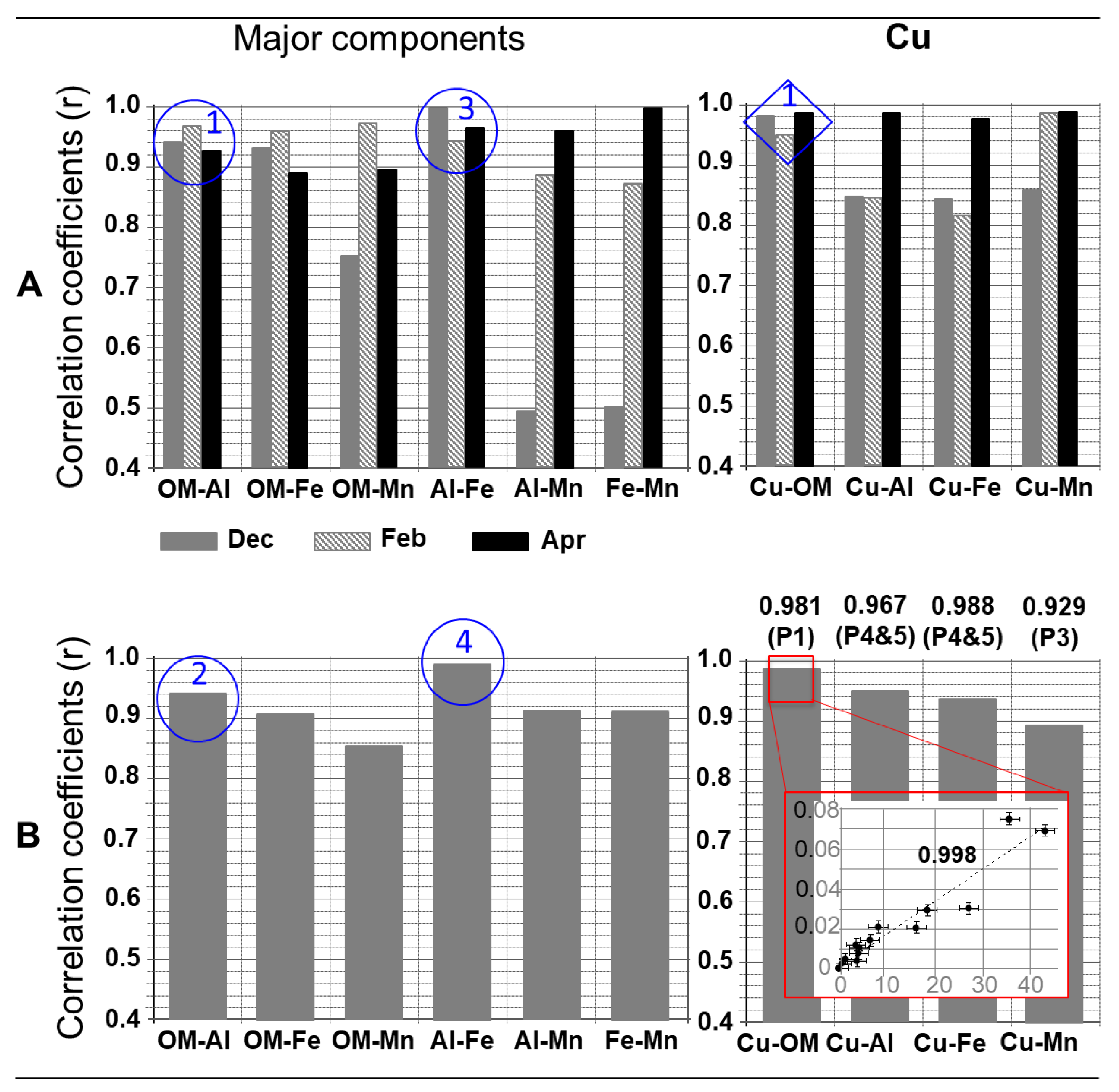
• P5, present in the April sample only, with the same components as P4. The concentrations of OM and Al correlated strongly (r = 0.938). The ratio of concentrations between these two components was also of the same order of magnitude (approximately 1/10) between P4 and P5. This suggests that P5 contained aggregates mainly consisting of the particles initially present in P4. This was consistent with the size distributions of these two populations (Figure 4).

Additionally, to Figure 4 and Table 1, Figure 5 presents the correlations established between the signals of the major components (A, left) and between their colloidal concentrations (B, left) and, similarly, the correlations concerning copper and the major components (A and B, right). This figure makes it possible, in particular, to complete the characterization of the different populations presented above.

Thus, the strong correlation (r > 0.93; Figure 5A, blue circle 1) between the OM and Al signals on the size continuum and between their concentrations (r = 0.947; Figure 5B, blue circle 2 and r > 0.987 specifically for P3 and P4) confirmed that these two components were strongly associated. The systematic presence of P3 and P4 also confirmed that non-labile clay-humic complexes were mobilized in the drain water. The strong correlation (r > 0.94; Figure 5A, blue circle 3) between the Al and Fe signals on the size continuum and between their concentrations (r = 0.988; Figure 5B, blue circle 4, and r = 0.998 specifically for P4) shows that there was also a strong association between clays and iron (hydr)oxides. Such a correlation was never observed between Al and Mn, Fe and Mn, and OM and Mn. On the one hand, their correlation coefficients varied significantly from one sampling month to another (Figure 5A). On the other hand, the correlation coefficients were lower for the concentrations than for the signals (r on the order of 0.90 for Al-Mn and Fe-Mn, and 0.85 for OM-Mn, Figure 5B). This suggests that manganese (hydr)oxides, with these other major components, formed complexes that were less stable (“less non-labile”) than those presented above, and/or that these complexes were less mobilized in the colloidal phase (the concentrations of Mn were generally lower than those of Fe; Table 1).

3.3. Copper Speciation

In the water of the monitored drain, copper was distributed (Figure 4, right) on P1 (12 to 21% depending on the month), P3 (3 to 9%), and P4 and P5 (76 to 79%), i.e., on populations where humic acids were (i) systematically and quantitatively present in free molecular form and/or in supra-molecular structures (P1), or (ii) complexed with inorganic particles (P3, P4 and P5). The Cu and OM signals correlated very strongly in all populations of all samples (r > 0.95; Figure 5A, blue diamond 1), as well as their colloidal concentrations (r = 0.981; Figure 5B, red square), and all of their concentrations in the dissolved-colloidal continuum (Figure 5B, red box). The correlations between Cu and the other major components are less important, varying according to their order of intensity, Cu-OM > Cu-Al > Cu-Fe > Cu-Mn. This trend is in agreement with the correlations between the major elements, notably OM-Al > Al-Fe > OM-Fe. All this shows the following:

• Cooper, in the colloidal phase, was very preferentially complexed with the soil humic acids during its mobilization towards soil water, and the complexes formed were non-labile. The copper present in the dissolved phase (<10 kDa) could be in free and/or labile forms. However, the correlation between Cu and OM (Figure 5B, red box) on the dissolved-colloidal continuum suggests that the predominant form of dissolved Cu was the form complexed with humic acids;
• Copper was also associated with clays and (hydr)oxides, mainly via clay-humic complexes ((Cu-OM)-clays using the notation in Figure 5) and complexes between (hydr)oxides and clays, taking into account the previous remark.

In the literature, it is shown that in acidic soils containing total copper concentrations of <10,000 mg kg⁻¹, copper is preferentially complexed with organic matter and, to a lesser extent, with clays [57,58,59]. The complexes, formed between Cu and organic matter, are of the internal sphere type [59]. The complexes formed directly between Cu and clays are of the outer sphere type and are sufficiently labile for the copper to remain easily mobilized [60,61,62]. In soil water, copper is generally found at more than 90% and is complexed with organic matter [63,64,65]. The observations made in the present study are consistent with the literature.

3.4. Copper Behaviour and Fate

During the preliminary study, the examination of the rainfall at the sampling times showed a correspondence between the water that fell with the total concentration of copper mobilized and transported by the water to the drain. In particular, copper appeared in all drains, approximately 15 to 30% more mobilized in the colloidal phase at the beginning of winter (which always followed a dry autumn during this study) than for the other samples.

There is little work in the literature quantifying the presence of copper in water in wine-growing areas. Bereswill et al. (2012) monitored different compounds including copper in several watercourses and runoff in wine-growing regions. They also considered rainfall, by monitoring an exceptional rainy episode following a 34-day drought; copper concentrations varied between the detection limit and 67 µg L⁻¹, with a median value of 5.4 µg L⁻¹ [66]. Although these concentrations are lower than those found in the present study, the authors highlight the observed dependence of copper mobilization and transport on rainfall.

In the present study, it rained very little during the 10 months preceding the monitoring of water from a drain, while between December and April, two periods of significant rainfall followed one another. The results obtained illustrate that the phenomena leading to the mobilization and transport of copper depend on the physicochemical conditions on the surface and in the soil, and that these conditions are governed by both the humidity level and the amount of water that fell and percolated the soil to the drain. Indeed, this dependence is reflected (i) by the sizes (in particular minimum) of the colloidal populations carrying Cu (except P1, essentially made up of humic acids of small sizes, less variable than those of particles) which slightly but systematically decreased between December and April (Table 1), and (ii) by maximum colloidal concentrations in December. This suggests the following:

• The first significant rains on dry soil probably had a preferentially mechanical action. The fragmentation of the soil, the genesis of particles including inorganic-organic composite colloidal particles carrying Cu, and their migration through the soil in the water flow to the drain, were the predominant mobilization and transport processes;
• The rains, even heavy at the end of winter/early spring, on soil that remained damp, probably had a preferentially chemical and physical action. The leaching and weathering of the soil caused the release of dissolved and colloidal organic matter to which copper is complexed, and the genesis of colloidal particles of a smaller size, overall, in less mass concentration but in higher particle number concentrations than in December. This favored the aggregation phenomena reflected by P5 and a more balanced distribution of copper between dissolved and colloidal phases.
• The transport of copper from the soil, via drain water, to the aquatic system must be considered spatially and temporally. Spatially, because taking into account the distribution of copper between the dissolved and colloidal phases, the transport of copper on a significant scale, particularly to river waters, is possible [16]. Temporally, because knowing that the drain water flows several hours after a rainy episode, or even for several days and weeks during rainy periods, a significant copper quantity can be transported. This quantity can be estimated from, on the one hand, the measured rainfall and the copper concentrations determined in drain water and drained surfaces, and, on the other hand, the total stock of copper in the soil (65 mg kg⁻¹ on average), considering that all the rain that fell infiltrated. Thus, during the rainy periods, around 3% per day on average of the copper stock could be transported outside the plots. At the maximum of the flow rates measured, up to 0.5% per hour of the copper stock could be transported. Given the alternation of dry periods / rainy episodes which promotes both leaching and weathering of soils, the quantities of copper transported in the long term are therefore indeed significant. This is in agreement with the observations of Bereswill et al. (2012). In their study, the copper contents in the surface sediments of watercourses were of the same order of magnitude as the concentrations in wine-growing soils studied [66]. This confirms that copper can be transported significantly, mainly in the colloidal form in our study, from vineyards to nearby river waters.

4. Conclusions

From an environmental point of view, the mobilization and transport of copper, from the soil to drain water, appears significantly linked to the original complexation in the soil of copper with organic matter. During rainy episodes, the mobilization of organic matter then takes the copper with it. This is either because the organic matter is directly released from the soil, or because soil particles containing organic matter are mobilized. Soil particles can contribute mainly to the presence of organic matter, and therefore copper, in water. The mobilization and transport of copper appear linked to rainfall in the following way: a dry period followed by a significant rainy episode favors the occurrence of copper in the colloidal phase, and a humid period followed by an intense rainy episode favors copper on a larger continuum due to aggregation phenomena. In all cases, the contrasting periods, in terms of variation of humidity, in the soil play a role in the soil and on the transport of part of its solid phase towards aqueous environments. In other words, soil erosion is promoted. This information appears particularly important in the context of climate change where these contrasting dry-wet situations are increasing in frequency and intensity. The quantities of copper transported are important compared to the total soil stock. This is all the more true as the soil must be considered as a recurring source of copper and as a source supplied by the treatment of the vines. Cu, even strongly attached to soil components, will therefore be released in the long term, and possibly in a more quantitative manner with the increase in the dry period-wet period contrast.

From a methodological point of view, all of this information was acquired by an investigation strategy based on the AF4-multidetection coupling and on the processing of the acquired data. By accessing the physicochemical speciation of copper, the occurrence of this element in drain water could be better evaluated and the influence of rainfall understood. In this, the approach followed appears relevant to meet the needs for environmental knowledge and management.

References

1. Lespes, G.; Zuliani, T.; Schaumlöffel, D. Need for revisiting the terminology about speciation. Environ. Sci. Pollut. Res. 2016, 23, 15767–15770. [Google Scholar] [CrossRef] [PubMed]
2. Tessier, A.; Campbell, P.G.C.; Bisson, M. Sequential extraction procedure for the speciation of particulate trace metals. Anal. Chem. 1979, 51, 844–851. [Google Scholar] [CrossRef]
3. Lespes, G. Nanoparticles in environment and health effect. In Metallomics: Analytical Techniques and Speciation Methods; Michalke, B., Ed.; Wiley-VCH Verlag GmbH & Co. KGaA: Markt Schwaben, Germany, 2016; Volume 11, pp. 319–337. [Google Scholar]
4. Lespes, G.; Faucher, S.; Slaveykova, V. Natural nanoparticles, anthropogenic nanoparticles, where is the frontier? Front. Environ. Sci. 2020, 8, 71. [Google Scholar] [CrossRef]
5. Lead, J.R.; Wilkinson, K.J. Environmental colloids and particles: Current knowledge and future developments. In Environmental Colloids and Particles. Behaviour, Separation and Characterisation; Wilkinson, K.J., Lead, J.R., Eds.; Wiley and Sons: Chichester, UK, 2007; Volume 10, Chapter 1; pp. 1–14. [Google Scholar]
6. Grolimund, D.; Barmettler, K.; Borkovec, M. Colloidal facilitated transport in natural porous media: Fundamental phenomena and modelling. In Colloidal Transport in Porous Media; Frimmel, F.H., von der Kammer, F., Flemming, H.C., Eds.; Springer: Berlin, Germany, 2007; pp. 3–27. [Google Scholar]
7. Hochella, M.F., Jr.; Mogk, D.W.; Ranville, J.; Allen, I.C.; Luther, G.W.; Marr, L.C.; McGrail, B.P.; Murayama, M.; Qafoku, N.P.; Rosso, K.M.; et al. Natural, incidental, and engineered nanomaterials and their impacts on the Earth system. Science 2019, 363, eaau8299. [Google Scholar] [CrossRef] [PubMed]
8. Lespes, G.; Gigault, J. Hyphenated analytical techniques for multidimensional characterisation of submicron particles: A review. Anal. Chim. Acta 2011, 692, 26–41. [Google Scholar] [CrossRef]
9. Ferreira da Silva, B.; Pérez, S.; Gardinalli, P.; Singhal, R.K.; Mozeto, A.A.; Barcelo, D. Analytical chemistry of metallic nanoparticles in natural environments. Trends Anal. Chem. 2011, 30, 528–540. [Google Scholar]
10. Zattoni, A.; Roda, B.; Borghi, F.; Marassi, V.; Reschiglian, P. Flow field-flow fractionation for the analysis of nanoparticles used in drug delivery. J. Pharm. Biomed. Anal. 2014, 87, 53–61. [Google Scholar] [CrossRef]
11. Maria, E.; Crançon, P.; Le Coustumer, P.; Bridoux, M.; Lespes, G. Comparison of preconcentration methods of the colloidal phase of a uranium-containing soil suspension. Talanta 2020, 208, 120383. [Google Scholar] [CrossRef]
12. Wahlund, K.-G.; Giddings, J.C. Properties of an asymmetrical flow field-flow fractionation channel having one permeable wall. Anal. Chem. 1987, 59, 1332–1339. [Google Scholar] [CrossRef]
13. Schimpf, M.E.; Wahlund, K.-G. Asymmetrical flow field-flow fractionation as a method to study the behavior of humic acids in solution. J. Microcolumn Sep. 1997, 9, 535–543. [Google Scholar] [CrossRef]
14. Baalousha, M.; Kammer, F.V.D.; Motelica-Heino, M.; Hilal, H.S.; Le Coustumer, P. Size fractionation and characterization of natural colloids by flow-field flow fractionation coupled to multi-angle laser light scattering. J. Chromatogr. A. 2006, 1104, 272–281. [Google Scholar] [CrossRef]
15. Bouzas-Ramos, D.; García-Cortes, M.; Sanz-Medel, A.; Encinar, J.R.; Costa-Fernández, J.M. Assessment of the removal of side nanoparticulated populations generated during one-pot synthesis by asymmetric flow field-flow fractionation coupled to elemental mass spectrometry. J. Chromatogr. A 2017, 1519, 156–161. [Google Scholar] [CrossRef] [PubMed]
16. Lespes, G.; de Carsalade du pont, V. Field flow fractionation for nanoparticle characterization. J. Sep. Sci. 2022, 45, 347–368. [Google Scholar] [CrossRef] [PubMed]
17. Schurtenberger, P.; Newman, M.E. Characterization of biological and environmental particles using static and dynamic light scattering. In Environmental Particles; Buffle, J., van Leeuwen, H.P., Eds.; Lewis Boca Raton: London, UK, 1993; Volume 2, Chapter 2; pp. 37–115. [Google Scholar]
18. Lespes, G.; Huclier, S.; Battu, S.; Rolland-Sabaté, A. Field flow Fractionation (FFF): Practical and experimental aspects. In Particle Separation Techniques: Fundamentals, Instrumentation, and Selected Applications; Handbook in Separation Science; Contado, C., Ed.; Elsevier: Amsterdam, The Netherlands, 2022; Chapter 19; pp. 621–657. [Google Scholar]
19. Hassellov, M.; Readman, J.W.; Ranville, J.F.; Tiede, K. Nanoparticle analysis and characterization methodologies in environmental risk assessment of engineered nanoparticles. Ecotoxicology 2008, 17, 344–361. [Google Scholar] [CrossRef] [PubMed]
20. Van der Horst, C.; Silwana, B.; Iwuoha, E.; Somerset, V. Spectroscopic and voltammetric analysis of platinum group metals in road dust and roadside soil. Environment 2018, 5, 120. [Google Scholar] [CrossRef]
21. Faucher, S.; Le Coustumer, P.; Lespes, G. Nanoanalytics: History, concepts and specificities. Environ. Sci. Pollut. Res. 2019, 26, 5267–5281. [Google Scholar] [CrossRef]
22. El Hadri, H.; Chery, P.; Jalabert, S.; Lee, A.; Potin-Gautier, M.; Lespes, G. Assessment of diffuse contamination of agricultural soil by copper in Aquitaine region by using French national databases. Sci. Total Environ. 2012, 441, 239–247. [Google Scholar] [CrossRef] [PubMed]
23. Flores-Vélez, L.M.; Ducaroir, J.; Jaunet, A.M.; Robert, M. Study of the distribution of copper in an acid sandy vineyard soil by three different methods. Eur. J. Soil Sci. 1996, 47, 523–532. [Google Scholar] [CrossRef]
24. Besnard, E.; Chenu, C.; Robert, M. Influence of organic amendments on copper distribution among particle-size and density fractions in Champagne vineyard soils. Environ. Pollut. 2001, 112, 329–337. [Google Scholar] [CrossRef]
25. Mc Kenzie, R.M. The adsorption of lead and other heavy metals on oxides of manganese and iron. Aust. J. Soil Res. 1980, 18, 61–73. [Google Scholar] [CrossRef]
26. Mc Bride, M.B. Forms and distribution of copper in solid and solution phases of soil. In Copper in Soils and Plants; Loneragan, J.F., Robson, A.D., Graham, R.D., Eds.; Academic Press: Cambridge, MA, USA, 1981; pp. 25–45. [Google Scholar]
27. Sauve, S.; Mc Bride, M.B.; Norvell, W.A.; Hendershot, W.H. Copper solubility and speciation of in situ contaminated soils: Effects of copper level; pH and organic matter. Wat. Air Soil Poll. 1997, 100, 133–149. [Google Scholar] [CrossRef]
28. Fernandez-Calvino, D.; Novoa-Munoz, J.C.; Lopez-Pezperiago, E.; Arias-Estevez, M. Changes in copper content and distribution in young old and abandoned vineyard acid soil due to land use changes. Land Degrad. Dev. 2008, 19, 165–177. [Google Scholar] [CrossRef]
29. Ma, Y.B.; Lombi, E.; Oliver, I.W.; Nolan, A.L.; McLaughlin, M.J. Long-term aging of copper added to soils. Environ. Sci. Technol. 2006, 40, 6310–6317. [Google Scholar] [CrossRef] [PubMed]
30. Anatole-Monnier, L. Effets de la Contamination Cuprique des Sols Viticoles sur la Sensibilité de la Vigne à un Cortège de Bio-agresseurs. Ph.D. Thesis, University of Bordeaux, Bordeaux, France, 2014; 199p. [Google Scholar]
31. Komárek, M.; Cadková, E.; Chrastný, V.; Bordas, F.; Bollinger, J.-C. Contamination of vineyard soils with fungicides: A review of environmental and toxicological aspects. Environ. Int. 2010, 36, 138–151. [Google Scholar] [CrossRef] [PubMed]
32. El Hadri, H. Pollution Diffuse des Sols par des Contaminants Minéraux et Impacts Environnementaux Liés aux Pratiques Agricoles. Ph.D. Thesis, University of Pau and Pays de l’Adour, Pau, France, 2012; 213p. [Google Scholar]
33. Harguindeguy, S.; Crançon, P.; Potin-Gautier, M.; Pointurier, F.; Lespes, G. Colloidal mobilization from soil and transport of uranium in (sub)-surface waters. Environ. Sci. Pollut. Res. 2019, 26, 5294–5304. [Google Scholar] [CrossRef]
34. de Carsalade du pont, V.; Faucher, S.; Lespes, G. Nanoparticles in waters and soil. In Field Flow Fractionation: Principles and Applications; Guegen, C., Baalousha, M., Williams, K.R., Eds.; Wiley-VCH: Weinheim, Germany, 2024; in press. [Google Scholar]
35. Dubascoux, S.; v d Kammer, F.; Le Hecho, I.; Potin-Gautier, M.; Lespes, G. Optimisation of asymmetrical Field Flow Fractionation for environmental nanoparticles separation. J. Chromatogr. A 2008, 1206, 160–165. [Google Scholar] [CrossRef]
36. El Hadri, H.; Gigault, J.; Chery, P.; Potin-Gautier, M.; Lespes, G. Optimization of flow-field flow fractionation for the characterization of natural colloids. Anal. Bioanal. Chem. 2014, 406, 1639–1649. [Google Scholar] [CrossRef] [PubMed]
37. Dubascoux, S.; Le Hecho, I.; Potin-Gautier, M.; Lespes, G. On line and off-line quantification of trace elements associated to colloids by As-Fl-FFF and ICP-MS. Talanta 2008, 77, 60–65. [Google Scholar] [CrossRef] [PubMed]
38. von der Kammer, F. Characterization of Environmental Colloids Applying Field-Flow Fractionation—Multi Detection Analysis with Emphasis on Light Scattering Techniques. Ph.D. Thesis, Technical University of Hamburg-Harburg, Hamburg, Germany, 2004; 234p. [Google Scholar]
39. Masson, M.; Guigues, N.; Arhror, M.; Raveau, S.; Brosse, C.; Forquet, N. Caractérisation de la Matière Organique d’Eaux Résiduaires et d’Eaux de Surface par les Sondes Spectrophotométriques UV-Visible; Research Report IRSTEA; Agence Française de la Biodiversité: Vincennes, France, 2019; 77p, hal-02609331. [Google Scholar]
40. Enev, V.; Pospisilova, L.; Klucakova, M.; Liptaj, T.; Doskocil, L. Spectral characterization of selected humic substances. Soil Water Res. 2014, 9, 9–17. [Google Scholar] [CrossRef]
41. Polak, J.; Bartoszek, M.; Sułkowski, W.W. Comparison of some spectroscopic and physico-chemical properties of humic acids extracted from sewage sludge and bottom sediments. J. Mol. Struc. 2009, 924–926, 309–312. [Google Scholar] [CrossRef]
42. Peacock, M.; Evans, C.D.; Fenner, N.; Freeman, C.; Gough, R.; Jones, T.G.; Lebron, I. UV-visible absorbance spectroscopy as a proxy for peatland dissolved organic carbon (DOC) quantity and quality: Considerations on wavelength and absorbance degradation. Environ. Sci. Process Impacts 2014, 16, 1445. [Google Scholar] [CrossRef] [PubMed]
43. Helms, J.R.; Stubbins, A.; Ritchie, J.D.; Minor, E.C.; Kieber, D.J.; Mopper, K. Absorption spectral slopes and slope ratios as indicators of molecular weight, source, and photobleaching of chromophoric dissolved organic matter. Limnol. Oceanogr. 2008, 53, 955–969. [Google Scholar] [CrossRef]
44. Chen, H.; Zheng, B.; Song, Y.; Qin, Y. Correlation between molecular absorption spectral slope ratios and fluorescence humification indices in characterizing CDOM. Aquat. Sci. 2011, 73, 103–112. [Google Scholar] [CrossRef]
45. Schimpf, M.E.; Caldwell, K.; Giddings, J.C. (Eds.) Field-Flow Fractionation Handbook; Wiley and Sons: New York, NY, USA, 2000. [Google Scholar]
46. Andersson, M.; Wittgren, B.; Wahlund, K.-G. Accuracy in Multiangle Light Scattering Measurements for Molar Mass and Radius Estimations. Model Calculations and Experiments. Anal. Chem. 2003, 75, 4279–4291. [Google Scholar] [CrossRef]
47. Teraoka, I. Polymer Solutions: An Introduction to Physical Properties; Wiley and Sons: New York, NY, USA, 2002. [Google Scholar]
48. Zimm, B.H. The Scattering of Light and the Radial Distribution Function of High Polymer Solutions. J. Chem. Phys. 1948, 16, 1093–1099. [Google Scholar] [CrossRef]
49. Bancon-Montigny, C.; Lespes, G.; Potin-Gautier, M. Organotin survey in Adour-Garonne Basin. Water Res. 2004, 38, 933–946. [Google Scholar] [CrossRef] [PubMed]
50. Masson, M. Synthèse Bibliographique sur la Faisabilité des Sondes Spectrophotométriques pour la Caractérisation In Situ de la Matière Organique; Report Aquaref; HAL: Lyon, France, 2015; 20p. [Google Scholar]
51. Faucher, S.; Ivaneev, A.I.; Fedotov, P.S.; Lespes, G. Characterization of volcanic ash nanoparticles and study of their fate in aqueous medium by asymmetric flow field-flow fractionation—Multidetection. Environ. Sci. Pollut. Res. 2021, 28, 31850–31860. [Google Scholar] [CrossRef] [PubMed]
52. Suraj, A.P.; Khalid, A.M.D.; Rajesh, K.; Asgar, A.; Yasmin, S. Humic acid from Shilajit: A physico-chemical and spectroscopic characterization. J. Serb. Chem. Soc. 2010, 75, 413–422. [Google Scholar]
53. McKnight, D.M.; Boyer, E.W.; Westerhoff, P.K.; Doran, P.T.; Kulbe, T.; Andersen, D.T. Spectrofluorometric characterization of dissolved organic matter for indication of precursor organic material and aromaticity. Limnol. Oceanogr. 2001, 46, 38–48. [Google Scholar] [CrossRef]
54. Ukalska-Jaruga, A.; Bejger, R.; Debaene, G.; Smreczak, B. Characterization of Soil Organic Matter Individual Fractions (Fulvic Acids, Humic Acids, and Humins) by Spectroscopic and Electrochemical Techniques in Agricultural Soils. Agronomy 2021, 11, 1067. [Google Scholar] [CrossRef]
55. Gale, B.K.; Srinivas, M. Cyclical electrical fiel flow fractionation. Electrophoresis 2005, 26, 1623–1632. [Google Scholar] [CrossRef] [PubMed]
56. Srinivas, M.; Sant, H.J.; Gale, B.K. Optimisation of cyclical electrical field flow fractionation. Electrophoresis 2010, 31, 3372–3379. [Google Scholar] [CrossRef] [PubMed]
57. Adediran, S.A.; Kramer, J.R. Copper adsorption on clay, iron-manganese oxide and organic fractions along a salinity gradient. Appl. Geochem. 1987, 2, 213–216. [Google Scholar] [CrossRef]
58. Mcbride, M.B. Reactions controlling heavy metal solubility in soils. Adv. Soil Sci. 1989, 10, 1–56. [Google Scholar]
59. Bravin, M.N. Processus Rhizosphèriques Déterminant la Biodisponibilité du Cuivre pour le Blé dur Cultivé en Sols à Antécédant Viticole. Ph.D. Thesis, Montpellier SupAgro, Montpellier, France, 2008; 237p. [Google Scholar]
60. Duchaufour, P. Introduction à la Science du Sol. In Sol, Végétation, Environnement, 6th ed.; de l’Abrégé de Pédologie; Dunod: Paris, France, 2001. [Google Scholar]
61. Hizal, J.; Apak, R. Modeling of copper(II) and lead(II) adsorption on kaolinite- based clay minerals individually and in the presence of humic acid. J. Colloid Interface Sci. 2006, 295, 1–13. [Google Scholar] [CrossRef] [PubMed]
62. Sposito, G. The Chemistry of Soils; Oxford University Press: Oxford, UK, 2008. [Google Scholar]
63. Bradl, H.B. Adsorption of heavy metal ions on soils and soils constituents. J. Colloid Interface Sci. 2004, 277, 1–18. [Google Scholar] [CrossRef]
64. Hodgson, J.F.; Lindsay, W.L.; Trierweiler, J.F. Micronutrient Cation Complexing in Soil Solution: II. Complexing Of Zinc and Copper in Displaced Solution from Calcareous Soils. Soil Sci. Soc. Am. J. 1966, 30, 723–726. [Google Scholar] [CrossRef]
65. Sauvé, S.; Dumestre, A.; Mcbride, M.; Hendershot, W. Derivation of soil quality criteria using predicted chemical speciation of Pb2+ and Cu2+. Environ. Toxicol. Chem. 1998, 17, 1481–1489. [Google Scholar] [CrossRef]
66. Bereswill, R.; Golla, B.; Streloke, M.; Schulz, R. Entry and toxicity of organic pesticides and copper in vineyard streams: Erosion rills jeopardise the efficiency of riparian buffer strips. Agric. Ecosyst. Environ. 2012, 146, 81–92. [Google Scholar] [CrossRef]
Figure 1. Preliminary study of copper over 2 years carried out in site drain waters (filtered at 0.45 µm) (n = 16). Concentrations are those of the dissolved and colloidal phases.
Environments 11 00019 g001
Figure 2. (A) Copper concentration over the dissolved-colloidal continuum of drain water collected in December, February, and April; (B) Monthly rainfall, superimposed with the colloidal concentration in drain water (in bold characters). LOD: 0.6 µg(Cu) L−1, 450 nm mentioned to define the fractions in the histograms (A) corresponds to the nominal sizes (cut-off threshold) of the filters used.
Environments 11 00019 g002
Figure 3. Typical UV-Vis spectra (A) of soil leachate measured for different sizes of the colloidal continuum (shown at 254 nm in (B)): Early peak (EP) and 100, 200 and 300 nm gyration diameters (A), and their associated spectral characteristics (C). EP corresponds to the peak eluted very quickly at the start of the fractionation (AF4), with a diameter of 15–20 nm at the peak top. For more details see the text regarding Figure 4 and Table 1.
Environments 11 00019 g003
Figure 4. Size distribution of major components and copper in the colloidal phase of the filtered drain waters, with the different populations identified according to their main composition (P1 to P5). OM from the UV-Vis detector, and Al, Fe, Mn, and Cu from ICP-MS.
Environments 11 00019 g004
Figure 5. Correlations between (A) the signals for each of the samples and (B) the concentrations in all the populations of all the samples, for the major components and copper whose distributions were presented in Figure 4. In addition, the concentration of Cu is plotted as a function of the concentrations of OM on the dissolved-colloidal continuum (concentrations expressed in mg L−1) (red box at the bottom right). All these coefficients were found statistically significant. For the details, see the text.
Environments 11 00019 g005