Abstract
Wastewater treatment plants (WWTP) play a critical role in mitigating adverse environmental impacts of urban and industrial wastewater by removing pollutants and reducing the risk of contamination. Discharges of treated effluents from WWTPs can still have significant effects on freshwater ecosystems, particularly on sensitive species like brown trout. We analyzed the effects of a modern WWTP on a freshwater ecosystem, studying fish biodiversity and biomass, the occurrence of the parasitic disease Proliferative Kidney Disease (PKD) on brown trout, river water temperatures throughout the year and fish habitat and diversity. No major differences between up- and downstream of the WWTP were observed in habitat structure and attractiveness, fish biomass and species diversity, nor in PKD prevalence or intermediate host presence. However, immediately at the WWTP’s effluent and continuing downstream, the water temperature rose by almost 1 °C. While WWTPs are crucial for reducing the environmental impact of urban and industrial wastewater, their effluents can still have important consequences for freshwater ecosystems. Brown trout are particularly susceptible to increases in water temperature, especially regarding PKD severity and consequent mortality. To ensure the long-term health and sustainability of freshwater ecosystems, it is imperative to improve measures to minimize water temperature rises and mitigate downstream cascade effects on sensitive organisms like brown trout.
1. Introduction
The continuing degradation of ecosystems increases the pressure on nature biodiversity [1]. Specifically, in aquatic ecosystems, declining biodiversity is obvious, and fish stocks are experiencing massive declines in marine and freshwater systems [2]. According to the Living Planet Index for Migratory Freshwater Fish, there has been a 76% average global decline in freshwater fish population from 1970 to 2016, with an even more pronounced decline of 93% of migratory fish in Europe [3].
Brown trout (Salmo trutta Linnaeus, 1758) is an excellent example of freshwater fish species experiencing huge declines for several decades, both globally and on a national scale in Switzerland [4,5,6,7]. Therefore, there is an urgent need to study environmental factors impacting aquatic ecosystems in general and especially freshwater fish, e.g., brown trout. Anthropogenic influences are the main factors impacting natural habitats and fish ecosystems in either a direct or indirect way. Primary causes for trout decline include habitat loss and degradation, overfishing, pollution, the introduction of non-native species, climate change and diseases [2,4,8,9,10]. For instance, Proliferative Kidney Disease (PKD) in brown trout is considered an emerging disease as it increases in severity with an increasingly warm climate and is expanding to new areas [11,12,13].
Brown trout is a species of freshwater fish that belongs to the salmonid family and is native to many countries in Europe. It is also found in parts of western Asia (Turkey and Iran) but has been introduced to other countries like North and South America and New Zealand, as it is a popular game fish. They have a distinctive appearance and inhabit several aquatic environments, preferably cold, clean and well-oxygenated waters, such as rivers, streams and lakes, and although some can undergo anadromous migration for spawning, others remain exclusively in freshwater throughout their lives. Those inhabiting rivers typically have a territorial behavior, and during the first years of their lives, they remain loyal to the territory where they hatched [14].
Some of the consequences of anthropogenic factors, like an increase in water temperature and a decrease in water quality, have immediate effects on fish health and immunity. Particularly, urbanization, dam constructions and land use changes result in reduced water quality and quantity and loss of suitable spawning and feeding areas for brown trout [9,15]. Water quality, for example, high levels of nutrients or low oxygen levels, has direct impacts on the fish’s immune system, making trout more susceptible to infections [16,17,18].
In aquatic ecosystems, water temperature is one of the most important environmental parameters controlling life, as fish and most other aquatic animals are poikilothermic animals, and their body temperature and metabolism are regulated by environmental temperature. Brown trout, as a cold-water-adapted species, is subject to the consequences of global warming, affecting their habitats and limiting life functions [19]. Besides these direct thermal effects, indirect effects, like the emergence of new diseases, also threaten the survival of this fish species [12,20,21].
Proliferative Kidney Disease (PKD) is a widespread disease that severely impairs brown trout health, causing high mortality events in wild populations [20,22,23]. It is caused by the myxozoan parasite Tetracapsuloides bryosalmonae, which alternates its life cycle between two hosts, comprising salmonid fish as a vertebrate and intermediate host; here, it is mainly young-of-the-year (YOY) brown trout; and freshwater bryozoa as invertebrate and obligate hosts. YOY represents the fingerling age category of brown trout, which is interesting for studying the disease, as it is their first encounter with the parasite. Usually, brown trout spawn in autumn, and the fertilized ova hatch in spring; the beginning of summer, with the rise in temperatures, is the time when they are the youngest in the stream of all trout. Older salmonids that have had previous contact with the parasite and survived the infection show immunity against re-infections in consecutive years or milder infections without mortalities [24]. Although no published data are available regarding other fish species’ role in PKD, our own observations have shown that other fish species could be potential accidental hosts disseminating parasite spores without clinical disease (Stelzer, unpublished data).
The disease is strongly temperature-dependent [4,25,26], and both hosts are subtle to environmental changes that have an influence on disease severity and spread [12]. Infective spores develop inside the bryozoan’s coelomic cavity [27] and are released into the river water. Fish become infected through gills, and the parasites enter the circulation and are distributed systemically, finally reaching the main target organ, the kidney. The parasite multiplies in the renal interstitium and differentiates to a sporogonic stage. It enters the renal tubules, where infective spores are released via urine until they encounter bryozoans and close the cycle. In trout, severe renal swelling gives rise to the name of the disease. Anemia and severe depletion of the hematopoietic tissue are clinical hallmarks of the disease, which cope with high mortality events [28]. Water temperatures above 15 °C exacerbate PKD severity and mortality [29]. This temperature has become a threshold and “risk temperature” for PKD in trout.
Pollution, such as from agricultural runoff or sewage discharge, can also negatively impact brown trout health by affecting water quality, food availability and the trout’s immune system. With the increase in human population, water contamination due to overpopulation, increase in land use and agricultural runoffs, wastewater treatment plants (WWTP) play a crucial role in managing and controlling water quality and pollution. Wastewater treatment plant techniques’ are constantly being improved, considerably reducing the waste that is excreted into the water bodies. However, a considerable impact of the WWTP and its effluents on environmental conditions is still present [30]. Many of the conventional WWTPs release micropollutants. These are emerging contaminants and comprise natural or synthetic substances and compounds of chemical elements that are found, i.e., in pesticides and wastewater from industry and hospitals. Also, sun creams, detergents, cosmetics, medicines and hormonal contraceptives contain micropollutants [31,32]. These substances can affect and alter fish health and fitness. The WWTP we examine in our study recently included a final step of ozonation to remove at least 80% of these micropollutants, together with a sand filter where breakdown products attach.
The structural and physical disruptions induced by WWTP effluents can resonate across the ecological spectrum, exerting consequences on riverine flora and fauna. Aquatic plants, crucial for stabilizing riverine habitats, are subject to direct influences and changes in sediment dynamics and substrate composition. The effects cascade to crustaceans and mollusks, both integral components of aquatic food chains. These interdependencies within river ecosystems ensure that alterations in one constituent reverberate throughout the food chain, affecting organisms at various trophic levels. Specifically, regarding PKD, bryozoan colonies, as living animals, are equally sensitive to habitat composition changes and water modifications [33,34,35].
Existing field studies on the effects of WWTPs on PKD usually only focus on one factor: the effects of WWTPs on the environment or on PKD or the effects of thermal impacts on disease. However, considering that fish health can be modulated by many factors simultaneously and that WWTPs can affect the ecosystem from different perspectives, a simultaneous analysis of multiple factors under the influence of WWTPs was needed to identify risk factors for fish population health and survival, e.g., fish habitat, PKD dynamics and pathology, bryozoan growth and water temperature.
The aim of this study was to analyze the effects of a modern WWTP on a freshwater ecosystem by studying:
(1) Fish biodiversity and biomass up- and downstream of the WWTP, (2) bryozoan occurrence, (3) PKD prevalence and associated pathology in brown trout, (4) river water temperature throughout the year, and (5) fish habitat structure and diversity.
We combined various methodologies to investigate the WWTP effects from different approaches, from the ecosystem level down to the molecular level.
2. Materials and Methods
2.1. Ethical Statement
This study was carried out in accordance with the University of Bern Animal Ethics Committee. Approval for animal experimentations was obtained from the Cantonal Veterinary Offices in Bern and Aargau, Switzerland (Authorization # BE102/14+ and # 75698).
2.2. Study Sites, Electrofishing and Brown Trout YOY Sampling
To calculate fish biomass and study fish diversity up- and downstream of the WWTP, fish upstream and downstream of the WWTP in the river Wyna (Switzerland) were electrofished. At two locations, we selected a river segment (102 m segment length upstream and 122 m segment length downstream of the effluent) (Figure 1), and all fish of all age categories were captured. The distance to the WWTP effluent of the upstream location was 242.50 m, and of the downstream location, it was 112.60 m. Fish numbers were counted by species, and they were identified based on their external morphological characteristics specific to the fish species. The total length was measured with a common ruler from the tip of the nose to the tip of the tail while the fish was lying on its side. Weight was measured with a common digital balance of 1 g accuracy (digital kitchen scale, Brabantia®, Valkenswaard, The Netherlands). The biomass was calculated as total kg per fish species in each segment.
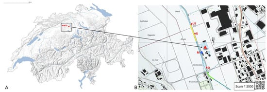
Figure 1.
(A) Map of Switzerland with location of the wastewater treatment plant marked as a red triangle. WWTP Coordinates: 47.2613388N, 8.171099E. (B) Location of sampling sites and temperature loggers along the river Wyna in canton of Aargau, Switzerland (© swisstopo). In bright green, the river segment that was fished upstream WWTP and where habitat quality measurement was performed. In yellow, the river segment fished downstream of the WWTP and where habitat quality measurement was performed. Red circle O: location of temperature logger 187 m upstream of the WWTP and eDNA sampling (2655437/1234702). Red circle M: location of temperature logger at the effluent and eDNA sampling (2655383/1234869). Red circle U: location of temperature logger 212 m downstream of the effluent and eDNA sampling (2655308/1235077). Red circle U1: location of temperature logger 500 m downstream of the effluent (2655272/1235181). Also included is the location of the wastewater treatment plant (WWTP, red triangle) and its effluent (blue-filled star). The coordinates of the segment upstream are 47.263020 N, 8.170012 E to 47.259923 N, 8.172160 E (102 m length), and the coordinates of the downstream are from 47.264247 N, 8.169385 E to 47.265842 N, 8.168600 E (122 m length).
To study T. bryosalmonae infection intensity, brown trout YOY at both locations were selected and euthanized by immersion in 150 mg/L buffered 3-aminobenzoic acid ethyl ester (MS 222®, Argent Chemical Laboratories, Redmond, WA, USA). Only YOY brown trout were selected for the PKD study, as it is the age category where they have the first contact with the parasite and the first infection takes place. Future infections of consecutive years can be either inapparent or not even take place and cause no pathological changes. Other species of fish in the river were not sampled for PKD analysis, as it is a disease that clinically affects only salmonid species, and brown trout are the only salmonids in this river. The disease occurs in the warm summer months, and the permission obtained from federal offices regarding fish samplings was given for only one sampling time point in the summer. Although we obtained very low fish numbers predominantly upstream, we did not obtain permission to repeat fish samplings due to the low numbers of young fish during that year in the river. A full necropsy was performed, and macroscopical changes in internal organs were annotated. The entire kidney was removed and cut longitudinally. One part was placed in RNAlater (Qiagen, Basel, Switzerland) and kept on ice before storage at −20 °C until further use for qPCR; the other half was placed in 10% buffered formalin for histopathological analysis.
2.3. Water Sampling
Based on the seasonality of PKD and the fact that the parasite can only spread when bryozoans reproduce, we chose sampling time points of river water close to the summer months and during the summer, which is when these events happen simultaneously. We sampled river water once monthly from April to October 2021 at three locations in the river (upstream “O”, downstream “U”, and at the effluent itself “M”) with a sterile 60 mL luer-lock BD PlastiPak™ syringe (BD (Becton Dickinson and Company), Franklin Lakes, NJ, USA) and a milipore Sterivex filter (0.45 µm pore size, Sterivex™, Merck KGaA, Darmstadt, Germany). The locations were coincident with the places where we placed three of the temperature loggers. Three water replicates (biological replicates) of 600 mL each were sampled at each location. In each location, a total volume of 1800 mL water was filtered on-site to retain environmental DNA (eDNA). The filters were closed on both ends of the cartridge with luer caps and kept on ice before storage at −20 °C until eDNA extraction. eDNA sampling locations are shown in Figure 1.
2.4. Bryozoan Optical Visualization
During the period of eDNA field sampling, field visualizations of bryozoans were performed three times: May, June and September. We aimed to detect their presence in these river localizations and selected the beginning and end of the warm months, as the beginning of the summer is the time when they reproduce and recolonize new river sites, and they are easier to visualize because they are more numerous. A segment up- and downstream of the water treatment plant was carefully observed for the presence of bryozoan colonies.
2.5. Histopathology
As a way to monitor pathological changes in brown trout, formalin-fixed kidney sections of brown trout were paraffin-embedded, cut into 4 µm thick slides and stained with Hematoxylin and Eosin (HE). All slides were evaluated under light microscopy (Nikon© Eclipse Ci-L plus, Tokyo, Japan). The presence of T. bryosalmonae was microscopically examined on whole histological kidney sections. The degree of infection (infection intensity corresponding to an estimation of the relative numbers of observed parasites per slide) and the severity grade of pathology were evaluated. To judge the degree of infection, a common score system was used [36]: 0 (no parasites present on the whole slide), 1 (single parasites), 2 (mild infection rate), 3 (mild to moderate infection rate), 4 (moderate infection rate), 5 (moderate to severe infection rate) or 6 (severe infection rate) at a magnification of 200 to 400×.
For the degree of kidney pathological alterations, the following changes were semi-quantitatively evaluated: hematopoietic tissue hyperplasia, loss of tubular structures, presence of granulomatous inflammation, formation of vascular thrombi with/without intralesional parasites, necrosis and presence of parasitic stages within interstitial tissue or within a renal tubular system. Histopathological lesions were graded from 0 (no renal pathological changes) to 6 (severe renal changes).
For each location, the histological grade and degree of parasitic infection, median value, and standard deviation for all examined fish per location (up- vs. downstream effluent) were calculated.
2.6. Quantitative PCR (qPCR) for Detection of T. bryosalmonae in Kidney Tissue and River Water
Kidney tissue: To analyze the parasite infection status of individual YOY brown trout, we performed a qPCR targeting a 435 bp fragment of the 18S rRNA gene of T. bryosalmonae. RNAlater fixed kidney tissue was used for DNA extraction, using a DNeasy blood and tissue kit following the manufacturer’s instructions (QIAGEN N.V., Venlo, The Netherlands). The amount and quality of DNA were measured on Nanodrop (NanoDrop One, ThermoFisher©, Waltham, MA, USA). qPCR was carried out according to [25]. The following primer/probe set was used: FWD primer (5′-3′)–GCGAGATTTGTTGCATTTAAAAAG, REV primer (5′-3′)–GCACATGCAGTGTCCA ATCG, probe (CAAAATTGTGGAACCGTCCGACTACGA). As a negative control, we used molecular-free water. We used an internal positive control of severely infected T. bryosalmoane-positive kidney tissue previously diagnosed in our laboratory.
River water: To study the presence of the parasite in the river water along the study river segments, eDNA from Sterivex filters was extracted without opening the housing, according to [37], with minor adaptations. The cartridge was inserted into a 5 mL tube without the hinge cap. To remove the remaining liquid in the filter, we centrifuged at 3059× g for 3 min. After centrifugation, we removed the 2 mL tube from the filter cartridge. A mixture of 80 µL proteinase-K solution, 880 µL PBS and 800 µL of buffer AL was added to the filter inside the cartridge. The cartridge was placed into a thermoshaker and incubated at 56 °C for 120 min at 200 rpm. After the incubation, the cartridge was inserted into a 5 mL tube, and these were inserted inside a 50 mL conical tube. A final centrifugation for 3 min at 3059× g was performed to collect the extracted DNA. The filter cartridge was removed with sterile forceps, and the 5 mL tube with the extracted eDNA was closed. The extracted eDNA was purified with a commercial kit (DNeasy PowerWater Sterivex Kit, Qiagen©, Hilden, Germany).
A qPCR was performed as described above for the detection of T. bryosalmonae on extracted water eDNA samples with the same primers and running conditions. Minor corrections were performed: an amount of 4 µL of eDNA sample was used per reaction, and there were 3 technical replicates/runs of each water sample.
2.7. River Water Temperature Measurement
To evaluate possible differences in water temperature up- and downstream of the WWTP, we placed temperature loggers (ONSET, Hobo ONS-U22-001) at four locations in the river (Figure 1): at the WWTP effluent itself (“M”, Coordinates: 2655383/1234869), approximately 187 m upstream the water treatment plant effluent (“O”, 2655437/1234702) and 212 m downstream the water treatment plant effluent (“U”, 2655308/1235077). A fourth temperature logger was located approximately 500 m downstream of the effluent (“U1”, 2655272/1235181). Temperature was recorded every 15 min between 20 April 2021 and 12 July 2022. The temperature loggers had to be removed from the water at this time point due to the time-limited permissions we obtained from federal authorities. For temperature analyses, we used HOBOware® Pro software (Version 3.7.25).
2.8. IAM—Habitat Quality Measurement
With the aim to evaluate habitat structure and its quality, we examined the same river segments as used for electrofishing. These characteristics influence the presence or absence of nutrients, fish and bryozoa, which are key factors for PKD dynamics. For this habitat evaluation, we used the IAM (Indice d’Attractivité Morphodynamique) method developed in the Swiss Jura region for trout-rich small-caliber rivers [38,39]. We performed the habitat assessment in autumn 2022, with fully developed vegetation and low water level.
The IAM is a method that describes the diversity of the river morphology and its attractiveness for the fish fauna. The method assumes that, under constant conditions regarding water quality and hydrology, the capacity of the water body for fish is determined by the diversity and attractiveness of the structural habitat. Habitat attractiveness can be quantified and calculated to the index IAMAST; this index correlates with the fish biomass resulting from quantitative fishing. Habitat diversity can be defined by the Shannon–Wiener Index HS.
For the distribution of depths and velocity classes, 10–15 cross-sections were surveyed in the investigated river sections at regular distance intervals of 10 m, in which points for flow velocity and water depth were recorded at 50 cm intervals along the cross-section, respectively. The following parameters were collected: the number of cross-sections, distance from the shore (in cm), depth (cm) and flow velocity (cm/s). In addition, the various habitats and their extensions were mapped.
All the data were then digitalized using the geographical information system QGIS (Software QGIS version 3.28.3). Interpolations were made between the points for water depth and flow velocity so that contiguous flow velocity and water depth patterns could be created for the two sections. The mapped habitats were also processed in QGIS (Software QGIS version 3.28.3) and assigned their attractiveness for fish. Habitats that offer good hiding places, such as undercut banks, deadwood accumulations, large boulders and aquatic vegetation, are considered particularly attractive, while mud, sand or rock are rated as less attractive. Attractiveness and types of all substrates are presented by [38].
In the end, four layers were created for the two studied sections: water depth (layer 1), water flow speed (layer 2), substrate/habitat (layer 3), overlay (layer 4).
The attractiveness index IAMAST is calculated and standardized from a combination of water depth, velocity, the number of substrates and the attractiveness of the substrates. It receives a value between 0 and an open-end value of >1.6.
For the calculation of habitat diversity, the first three layers are overlaid (in layer 4). This creates areas that are composed of the substrate, depth and flow speed attributes. This fourth layer is used for further calculations of habitat diversity. The diversity index is then calculated with the Shannon–Wiener Index [40]. This index is a mathematical measure for describing diversity. The diversity index receives a value between 0 and an open-end value >1.32.
This habitat quality measurement is combined with fish biodiversity of the same river segments for interpretation of the results.
2.9. Statistical Analysis
Statistical analyses and graphical presentations were carried out using R (version 4.3.1) [41,42]. During the analysis, we used packages “ggplot2”, “devtools”, “ggpubr”, “dplyr”, “rlang”, “vcd”.
In the first approach, we evaluated whether our datasets (histological score, parasite load score and water temperatures) were normally distributed using histograms and Shapiro–Wilk tests. We evaluated the data distribution for the temperatures in each sensor using the “average of temperatures per day”. The Shapiro–Wilk tests confirmed that our data are not normally distributed in any of our datasets.
Afterward, we performed the Mann–Whitney–Wilcoxon test (also referred to as Wilcoxon rank sum test or Mann–Whitney U test) to verify that all datasets are independent (this test is the non-parametric equivalent to the Student’s t-test for independent samples). We added box plots to graphically visualize histopathological scores against parasite load.
For the water temperatures, we performed this test to understand if the statistic temperatures differ between the different sensors.
We used several approaches to analyze the temperature differences between the logger locations. In theory, we have 4 time series datasets without repetitions in 15 min intervals. First, we analyzed the whole dataset of the whole study period; secondly, we performed daily and monthly temperature means. Later, we studied the variations in time series datasets (one per logging location): we performed the first difference (subtracting the previous values from each), 8 h difference and 12 h difference. We incorporated new variables such as the “risk” value and “exposure time”. For “Risk”, we divided the temperature ranges into the following categories: “null” if below 14 °C, “low” if temperatures were between 14 and 15 °C, and “high” if temperatures were above 15 °C. This served to analyze the correlations of the different temperatures between the locations. “Exposure time” represented the cumulative time in minutes above 15 °C in each location. Even after these data transformations, we could not correlate the location with histological score and parasite load due to the low sample size and the distribution of the samples.
3. Results
3.1. Fish Biodiversity and Biomass
To compare river sites regarding fish biodiversity and biomass, all fish in both segments were fished, counted and measured. Downstream of the treatment plant effluent, there were fewer fish, but a higher biomass was recorded in comparison to the upstream location (Table 1). This is due to inhabiting fish having a greater ratio of body surface to weight, meaning they were bigger than in upstream segments.

Table 1.
Results from the electrofishing regarding fish biodiversity and calculation of fish biomass after length and weight measurements. Represented are the fish species found in the up- (A) and downstream (B) segments and their total numbers. The calculation of the total number/ha is based on the number of fish encountered in the sampled river segment and extrapolated to one hectare of river surface. The taxonomic authority of all Latin names is Linnaeus, 1758. 1 From [43].
Regarding individual fish species, European bullheads (Cottus gobio, Linnaeus 1758) were more represented compared to European chubs (Squalius cefalus, Linnaeus 1758) and common minnows (Phoxinus phoxinus, Linnaeus 1758) in the downstream location. Interestingly, brown trout were equal in number at both sites of the WWTP. However, as the site downstream of the WWTP was longer than the upstream site, the calculation of the theoretical relative biomass of all fish species, including brown trout, is higher upstream. Common barbels (Barbus barbus, Linnaeus, 1758) were only present, even if in low numbers, in the downstream site; stone loach (Barbatula barbatula, Linnaeus, 1758) was barely represented, with only one individual in the upstream site (Table 1).
3.2. Brown Trout Sampling and Necropsy Findings
For the evaluation of PKD, we fished all YOY brown trout present in both river segments. Fourteen brown trout YOY downstream and five YOY upstream of the water treatment plant effluent were examined. Downstream, eleven out of fourteen trout showed macroscopical changes suggestive of PKD, while upstream, three out of five fish showed lesions compatible with PKD, ranging from enlargement of kidney tissue to visible white nodules on the surface.
3.3. Bryozoan Visualization
To analyze the presence of bryozoans in up- and downstream locations of the WWTP effluent, we performed three visual inspections throughout the study period of both river segments. None of these inspections revealed bryozoan colonies.
3.4. Histopathological Assessment
To evaluate the severity of infection, parasite load and incidence of PKD, we studied renal tissue from the necropsied YOY brown trout and performed semi-quantitative evaluations of histopathological lesions and parasite intensity scores. At both sites of the WWTP, parasite infection induced microscopic alterations of the kidney compatible with PKD infection. The median kidney histopathology score downstream was 2, with a standard deviation (SD) of 1.9. At the upstream location, the median histopathology score was 0, with an SD of 2.5. Here, three of the five animals analyzed had no histopathological changes, and two had a high score of 4 and 5, with moderate to severe lesions in the renal tissue (Table 2). In summary, the histopathological score differed between locations in a way that the median value of downstream fish was 2 and upstream was 0, as three out of five animals did not show any histological lesions; however, the other two fish had high scores of 4 and 5 (Figure 2).
Table 2.
Overview of the young of the year brown trout, Salmo trutta (Linnaeus, 1758), sampled for Proliferative Kidney Disease analysis from the river Wyna, Switzerland on 18 August 2021. Prevalence of Tetracapsuloides bryosalmonae, as indicated by qPCR from fish kidney samples, was 100% for all fish captured. Kidney histopathological score and parasite load are given as means ± standard errors and the range in brackets. Abbreviations: WWTP—wastewater treatment plant; BCI—body condition score, as determined as the ratio of body weight to body length; n—number of brown trout captured from each location.
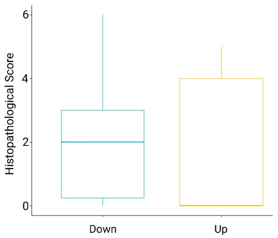
Figure 2.
Boxplot of Histopathological scores of Proliferative Kidney Lesions for brown trout (Salmo trutta, Linnaeus 1758) kidney samples from up- (yellow) and downstream (blue) locations of the WWTP in the River Wyna, Switzerland, 2021. Range of pathological lesions from 0 to 6, in ascending order of severity. Sample sizes were downstream n = 14 and upstream n = 5, with three upstream fish showing no pathological changes (0) and downstream fish scores ranging from 0 to 6, with the majority of fish having a score of 2.
Regardless of their sampling location, the twelve fish with kidney histological lesions showed different degrees of inflammation and parasite load. The main histological findings were compatible with acute or chronic active renal changes consisting of accumulations of macrophages within the interstitium (granulomatous inflammation), the proliferation of interstitial tissue, hematopoietic hyperplasia, loss of tubular structures, and the presence of intratubular and interstitial extrasporogonic myxosporidian parasites. Occasionally, intravascular thrombi composed of parasite stages and fibrin, and mainly macrophages and a few lymphocytes were seen. Parasites were detected in the renal interstitium, in the vessels and also in the tubular lumen. No signs of other diseases were present.
In total, seven fish did not show histopathological changes in the kidneys suggestive of infection with T. bryosalmonae, although one of them showed parasites within the interstitium with no associated lesions. The parasite load downstream had a median score of 1.5 with an SD of 1.7, and upstream, the median score was 1 with an SD of 2.8; fish had either no or high amounts of parasites.
When comparing the parasite load with the histological score of the renal lesions, we found a significant linear correlation between these two variables (Figure 3). This means that the parasitic load is correlated with the histological lesions and vice versa at both sampling sites.
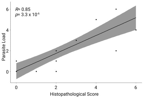
Figure 3.
Scatter plot of the Pearson’s correlation of parasite load and histopathological score of all sampled fish. The R score was close to 1, and the p-value < 0.05, which means that there is a significant correlation between these two variables.
3.5. T. bryosalmonae Prevalence in Fish
To verify the prevalence of trout positive for T. bryosalmonae, we performed a qPCR. There was a 100% prevalence of infection above and below the WWTP.
3.6. eDNA for T. bryosalmonae
We additionally tested parasite presence through eDNA of river water samples. In general, the detection of eDNA towards T. bryosalmonae was low. However, we could detect parasitic eDNA at least twice in all sampling locations between May and October. In July, samples were positive up- (O) and downstream (U) of the effluent simultaneously. The Ct values of the qPCR results were always high (between 35 and 48). In most of the samples, only one technical replicate (qPCR replicate) and one water replicate (biological replicate) were positive. Only in June, all three technical replicates in the qPCR run from the downstream location U were positive for parasitic DNA (Figure 4).
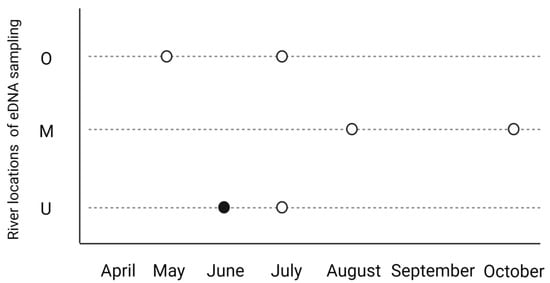
Figure 4.
eDNA results of parasitic DNA in the water at the three river locations during the sampling period. Spheres represent samples that were positive for T. bryosalmonae in eDNA samples in the qPCR for T. bryosalmonae. White spheres are those where one technical replicate was positive. The black sphere is one water sample where all qPCR technical replicates were positive. In total, we detected parasitic eDNA during this period two times in each location. Abbreviations: O—187 m upstream effluent; M—at the effluent; U—212 m downstream the effluent.
3.7. Temperature Measurements
Temperature records throughout the study period served to identify possible differences in river water temperatures and presumptive risk factors between up- and downstream sites. Indeed, there were notable differences between the upstream location compared with the other three sampling sites (details of the summer river temperatures are in Table 3).
Table 3.
Water temperature recorded in the River Wyna, Switzerland, during warm months and Summer of 2021 at sites in proximity to a wastewater treatment plant (WWTP). Values are reported as means ± standard errors, with temperature ranges provided in parentheses for each sampling location and date. Sampling locations: O—187 m upstream from WWTP, M—at WWTP effluent discharge point, U—212 m downstream from WWTP, U1—500 m downstream from WWTP. Mean temperatures that exceed the threshold for Proliferative Kidney Disease (PKD) in brown trout (Salmo trutta Linnaeus, 1758) of ≥15 °C are indicated in bold text with an asterisk (*).
The yearly average temperatures at the four river locations differed by at least 0.94 °C between upstream (O) and the other three locations (M, U and U1), with O being the location with the coolest average temperature throughout the year.
In general, the effluent site (M) was revealed to be the location with the highest temperature. The temperature of the water remains similar through the following 500 m, and in the last location, U1 (500 m after the effluent), the water temperature is still higher compared to upstream of the effluent (Table 4). The number of consecutive days where the temperature reached peaks over 15 °C was higher compared to the number of days where the average temperature reached ≥15 °C.
Table 4.
Overview of average temperature differences between locations with special attention to the 15 °C threshold. Average temperatures between the locations differ considerably between O and the other three locations (M, U and U1). Between the upper location (O) and the last downstream location (U1), which covers 687 m, there is almost 1 °C difference in yearly average temperature. The count of days where average temperatures reached ≥15 °C is clearly less in the upstream location compared to the other three locations. As 15 °C is a critical temperature cutoff for PKD outbreaks and mortalities, this temperature difference between up- and downstream of the WWTP effluent is a considerable risk for trout inhabiting downstream sites of the WWTP.
Even though all logged river sites showed temperatures ≥ 15 °C between June and August, in all sites downstream of the WWTP effluent, the number of consecutive days and weeks and the overall number of days with extreme temperatures is clearly higher compared to the upstream site (see Figure 5).
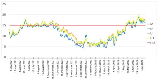
Figure 5.
Graphical representation of daily average temperatures throughout the complete study period with data from all temperature loggers. The red line (risk) represents the cutoff value of 15 °C temperature, which is critical for PKD in trout. Daily average temperatures from all loggers were calculated, and each color represents one temperature logger. As visible, during the summer months, the temperatures were above the red line for many consecutive days and weeks. Regarding the loggers, the water in the upstream location was always cooler compared to the other three locations. Abbreviations: Aug—August; Sept—September; Oct—October; Nov—November; Dec—December; Jan—January; Feb—February.
The monthly average temperature in June, July, August and September was above 15 °C in all the locations (M, U and U1) except in the location upstream of the effluent (O) (see Table 5). The locations M, U and U1 can be grouped together for the comparison with O, as they show very similar temperature regimes, while the difference of them with O is generally very clear (see details in Table 4 and Table 5).
Table 5.
Total number of days with daily mean water temperatures ≥ 15 °C at each location and the monthly average temperature per location. Months where temperatures reached the 15 °C cutoff. For each temperature logger, days within each month that reached that temperature are summed up. Mean temperatures for each month, for each logger, were calculated. The upstream location O was revealed to have fewer days ≥15 °C compared to the other three locations. The effluent itself, M, has the highest temperatures and number of days above 15 °C, and within the next 500 m, until the last logger U1, the temperature has not recovered to temperatures from upstream the effluent. The critical water temperature for PKD development, related clinical signs and mortality in trout is 15 °C.
The distribution of temperatures between May and August 2021 was different between upstream and downstream: we observed that upstream of the WWTP, the majority of temperatures measured lies below 15 °C, whereas at the effluent and further downstream, the majority of temperatures lies above the 15 °C threshold (Figure 6). Temperatures were very slightly different between the effluent and further downstream sites (M and U, U1), so we chose the logger at the effluent for this comparison.
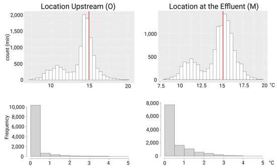
Figure 6.
Histograms showing the temperature distribution in minutes (top) and frequency (bottom) in upstream location (O) and at the effluent (M). Temperature was logged every 15 min, and histograms on the top show the count of the 15-min intervals. Upstream, the majority of the measured temperatures lies below 15 °C, whereas at the effluent, the majority lies above the PKD risk temperature of 15 °C. The red line represents the risk temperature of 15 °C for Proliferative Kidney Disease. The lower histograms depict the frequency of temperatures exceeding 15 °C within 0.5 °C intervals. Abbreviations: min—minutes; O—logger upstream; M—logger at the effluent.
Regarding daily temperature variations between the different sites, we detected high variabilities, predominantly between O (upstream) and the other three loggers. When we compared upstream temperatures with the other locations, the temperature followed a similar pattern of variability between O and M, O and U, O and U1, with O always being cooler than the others. Daily variations range between 0.5 and 1 °C most of the time, reaching even peaks of almost 2 °C.
In our case scenario, the Mann–Whitney–Wilcoxon test resulted in statistical significance between the logger upstream (O) vs. the other three (M, U and U1) and with no statistical difference between the temperatures measured in all loggers from the effluent downstream (M, U and U1) (Table 6). The average temperature of each day differs by almost 1 °C between up- and downstream sites, and this difference represents a strong biological risk because this 1 °C difference occurs exactly between 14 °C and 15 °C water temperature (the risk temperature for PKD).
Table 6.
Analysis of variability between the different temperature measurement locations and the resulting p-values of the Mann–Whitney–Wilcoxon test. With an asterisk and in bold are the p-values that show statistical differences, with the comparison between upstream and all downstream locations always being significantly different and the downstream sites with each other without statistical differences. Abbreviations: O—logger 187 upstream of the WWTP effluent; M—logger at the effluent; U—logger 212 m downstream of the effluent; U1—500 m downstream of the effluent.
3.8. Indice d’Attractabilité Morphodynamique (IAM): Habitat Quality Measurement
To analyze the attractiveness of the river morphology for fish and the habitat diversity in both river segments, we used the IAM technique. The upstream location reached an IAM score of 0.56 (unattractive), and the downstream location was 0.98 (moderately attractive).
Based on these data, the attractiveness status at both sites appears to be low to moderate, as indicated by the IAM scores. Additionally, there is a small difference between the two sites.
The river segment upstream of the WWTP has a reduced attractiveness for fish and high habitat diversity: The habitat diversity (HS) upstream of the WWTP is categorized as high (1.30) due to the presence of many different substrates (11) and especially due to the presence of four out of five different water depth classes, which leads to a higher variability. The substrate is composed of 71% of clogged stones (GLS), followed by 9% of big stone blocks (BLO). The remaining substrates are clogged gravel (GRS), some bankside vegetation (HEL), gravel (GRA), fine sediment (FIN) and organic litter (LIT), among others, with varying frequencies between 6% and 1% (see Figure 7A). However, the number of unattractive substrates for fish, like clogged stones or blocks, is much higher than attractive substrates such as bankside vegetation, deadwood (BRA) or washed-out banks (BER).
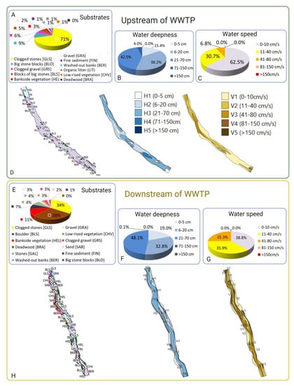
Figure 7.
Analysis of habitat quality and diversity in river segments up- and downstream of the WWTP effluent with IAM method [38,39]. (A–D) Segment upstream. (A) Percentage of the different substrates present in the segment upstream. The vast majority of the segment is covered by clogged stones (71% of the surface) and 9% of big stones, so 80% of the segment is composed of unattractive substrates for fish. Attractive substrates like bankside vegetation, deadwood and washed-out banks are not more than 4% of the segment. (B) Water depth had a moderate variability, with 4 different water depth classes being present; the majority of the segment surface had depths of 6 to 70 cm. A very low percentage of 4% had deeper parts of more than 70 cm, which are suitable for adult fish. (C) Water speed was overall low, and only three speed categories were present, with the majority of the segment (63%) showing speeds of 0 to 10 cm/s and the rest of the segment up to 80 cm/s. Fast-flowing sections were missing, which would be suitable for strong swimming fish. (D) Mapping of the substrate, flow and depth layers in the upper section of the river. (E–H) Segment downstream. (E) Percentage of the different substrates in downstream segment is represented. The variability of substrates is high; the quantity of attractive ones is low to moderate but still higher than the upstream segment. More than 50% is covered by clogged stones and big clogged stone blocks, both unattractive substrates for fish. Presence of bankside vegetation (11%) and deadwood (7%) and washed-out banks (4%) increases the attractivity of this segment compared to upstream. (F) Water depth classes are only three, with low water depths of up to 70 cm. Deeper parts are completely missing. (G) Water speed also only included three classes upstream; they were more or less equally distributed between low and moderate. Again, fast-flowing sections were missing, which would be suitable for strong swimming fish. (H) Mapping of the substrate, flow and depth layers in the downstream section of the river.
Water depth was predominantly (42.5%) from 21 to 70 cm (class 3), followed by depths of 6 to 20 cm (class 2) in 38.2% of the river segment. The remaining zones were from 71 to 150 cm depth (class 4; 4%) or 0 to 5 cm (class 1; 15.4%) (Figure 7B).
The water speed was low in most of this river segment, with 0–10 cm/s (class 1) in 62.5% of the segment. A low to moderate speed of 11–40 cm/s (class 2) was found in 30.7% of this river segment, and a moderate speed of 41–80 cm/s (class 3) was found in in 6.8%. Fast-flowing sections for strong swimming fish were not present (Figure 7C).
Downstream of the WWTP, the river segment has a high diversity of habitats but not a high quality. The habitat diversity (Hs) of the downstream segment is very high, with 1.59. There are, in total, 12 different types of substrates. Of those, more than half are composed of unattractive clogged stones (38.8%, (GLS)) and blocks of big clogged stones (28%, (BLS)). The majority of the remaining substrates are attractive for fish and range between 11% and 0.4%; they are composed of bankside vegetation (11%, (HEL)), deadwood (7%, (BRA)), stones (4%, (GAL)), undermined riverbank (4%, (BER)), gravel (3%, (GRA)), low vegetation (3%, (CHV)), sand (2%, (SAB)) or fine sediment (1%, (FIN) (Figure 7E).
Water depth had a medium variability, as three out of five different depth classes were present. Most of the segments were 21–70 cm (class 3, 48%). A high proportion was 6–20 cm depth (32.8%), and 19% was 0–5 cm deep (Figure 7F). Deeper sections with more than 70 cm water depth, which would be attractive, especially for adult fish, were missing.
The water speed scores were distributed between three categories out of five: 38.8% had a low speed of 0–10 cm/s (class 1). A total of 35.9% had a low to moderate speed of 11–40 cm/s (class 2), and 25.3% had a moderate speed of 41–80 cm/s (class 3). Fast-flowing sections, which would be suitable for strong swimming fish, such as adult trout or barbel, were also missing, like in the upstream segment (Figure 7G).
4. Discussion
In this study, we assessed the impact of a WWTP on various factors in the complex interplay of environment, pathogen and host. The evaluation of environmental pollution typically concentrates on the effects at medium to large scales [44,45], sometimes neglecting the significance of small-scale effluent discharges on natural environments. This study focuses on examining the small-scale impacts of WWTP effluent, how subtle differences in ecological quality can result in big impacts on the environment, and how they contribute to habitat deterioration and PKD dynamics, specifically from the standpoint of the fish host.
In August 2021, when we performed the fish sampling, we encountered a natural limitation for our study, which was a low sample number predominantly upstream of the effluent. Only five brown trout of our age category of interest for PKD (YOY brown trout) were present in that river segment. This is probably due to winter floodings destroying brown trout spawning sites and reducing considerably the number of young trout that year. This constraint has limited our evaluations and statistical analyses.
Given the variability of environmental conditions across distinct geographical locations within natural settings, the establishment of an authentic control site within the framework of our study design was not possible. Consequently, we opted to designate a segment of the river situated upstream from the WWTP as our reference site, wherein the impact of wastewater influence is either absent or notably reduced. For future studies, it would be useful to include another sampling site further upstream of the WWTP to avoid the possible influence of migrating fish.
Our hypothesis was that WWTP effluent influences the presence of PKD in trout through direct or indirect effects on the environment. To test this, we analyzed (i) WWTP impacts on river ecomorphology, including fish biomass, diversity and attractiveness of river sites for fish; (ii) presence of the bryozoan host; (iii) T. bryosalmonae presence in trout kidney and its effects in trout kidney (histological score and parasite load); and (iv) spatiotemporal temperature differences immediately upstream, downstream and directly at the WWTP effluent with its effects on fish PKD/health status.
Considering the limitations of the small fish sample size we had in the upstream location (n = 5) and the values of the histopathological scores and parasite loads, we detected a bias in the dataset towards more disease and more parasite exposition in downstream sites, but statistically, we cannot conclude that these parameters are correlated with the sampling location.
When taken together, our results show subtle differences regarding some parameters studied, indicating that the presence of a WWTP, even a modern plant that eliminates most of the micropollutants, has influences on a river ecosystem with indirect effects on fish health.
In our study, we found a temperature increase of almost 1 °C of the river water at the WWTP effluent that could have massive effects on a natural riverine environment, and its range covers the critical temperature of 15 °C, which is crucial for PKD dynamics and known to be detrimental for trout health. PKD is a dynamic disease dependent on several factors, while one key factor is increasing temperature [12,26,29]. Outbreaks are additionally temperature-dependent [46,47], and reaching or exceeding the threshold temperature of 15 °C results in massive mortality events [4,20], compared with habitats where the temperature remains below 15 °C, where fish can host the parasite without clinical signs. With the temperature rise, habitats suitable for the disease are expanding. In a field study on wild brown trout populations, Rubin et al. developed a model to identify possible disease hot spots. They identified temperature increase as the most important parameter correlated with the prevalence and infection intensity of T. bryosalmonae [11,48]. Mathematical models over the past half century have shown that even very slight increases in water temperature, as seen in our study, have critical impacts on ecological temperature thresholds with effects on the spread of fish diseases [49]. The same applies to models for future temperature scenarios, like those expected for the end of this century, which explain the catastrophic effects of temperature increase on ecological systems, especially on salmonid populations [50]. River temperature conditions will be favorable for the spread of PKD in Swiss plateau rivers. In trout, metabolism and immune system are temperature-dependent [19]; therefore, surrounding water temperature plays a crucial role in disease development. The increase in temperature from the effluent downstream is visible across the whole study period and across all studied variables (yearly mean, monthly means, and daily variations in temperatures). Although we cannot discuss significant differences between the temperatures in the different locations, as already observed, the locations from the effluent downstream are exactly at the threshold of 15 °C, which is critical to PKD. Even without statistical significance, the biological significance of this 1 °C difference between up- and downstream sites can have big implications for this disease dynamics, turning the WWTP in our study system into a pivotal player.
Even at low concentrations, we detected parasitic eDNA in all examined locations. eDNA is a fantastic non-invasive tool for pathogen detection and/or monitoring [51]. It has been successfully applied to detect different diseases, like Aphanomyces astaci [52], Batrachochytrium dendrobatidis [53] or Flavobacterium psychrophilum [54]. The authors of [55] determined that the presence of T. bryosalmonae eDNA was influenced by spatial factors [56]. The detection of the agent through eDNA relies on the concentration and dispersal of the target DNA at a specific location [57]. Conducting eDNA studies involves various challenges, such as determining the origin, state, transport and fate of the DNA in the environment [58]. As eDNA tends to remain in proximity to its production source, this can result in the absence or very low concentrations of target DNA in samples collected outside of “hotspots” [59,60,61]. In cases where target DNA is present, the concentrations may be close to or below the limit of detection. Nevertheless, some authors argue that even if PCR detections from eDNA are below the limit of detection, they could still be valid positives with meaningful implications, albeit with a lower level of reproducibility than desired [62]. In our study, bryozoan hotspots were at unknown sites, and our results have manifested in general low detection rates. Therefore, eDNA samples for T. bryosalmonae analysis are less reproducible. Interestingly, only in July were two locations positive for the parasite at the same time, a time point that coincides with bryozoan blooming (enhanced growth) [46,56,63].
As our eDNA measurements revealed positive results for the parasite in all locations, both bryozoans and T. bryosalmonae exist down- and upstream of the WWTP. Many studies show that WWTPs are major point sources in the enrichment of surface waters [64,65]. As previously shown, bryozoans respond to increasing nutrient concentrations by increased growth, which results in higher biomasses in enriched waters [63].
In this river segment, no mechanical barriers are present that could affect fish migrations from the down- to the upstream segment. Therefore, we cannot completely exclude possible migrations of trout. The two fish from the upstream segment that showed high parasite load and histological scores could thus have migrated from the downstream site. Nevertheless, brown trout exhibit site fidelity to their site of hatching and manifest distinctly territorial conduct during their initial years of development. To ensure absolute accuracy, a future investigation should undertake fish samplings at incremented intervals upstream from the wastewater treatment plant effluent.
We explored habitat structure and quality, fish biodiversity and biomass to analyze environmental quality and degradation. We aimed to understand if the WWTP implementation with its effluent was affecting the river structure itself with influences towards fish and possibly bryozoan growth. Bryozoan species like well-oxygenated waters with a constant and mid-strong water flow and with places to colonize like deadwood, conglomerate stones or even plastic. According to this, both river segments were rather inappropriate for bryozoan colonies regarding the structure, but downstream water speed was more favorable for bryozoan growth. Also, fish biodiversity and biomass were increased in the downstream location compared to the upstream location, as was the habitat quality measurement. The presence of barbels in the downstream site is also a biological indicator for better current variability, as they are adapted to areas with fast-flowing water. The same applies to adult fish like brown trout, who prefer river places with higher water currents. Fish abundance and variability reflect a habitat’s quality, and as such, they cope together with our findings of the habitat assessment: the habitat was more attractive and diverse for fish in the downstream location. Globally, there are few rivers that are left intact from human action [66]. Higher water temperatures, like those downstream of the WWTP effluent, are linked with more nutritional resources for invertebrates and, directly and indirectly, for fish. Apart from the better habitat structure for fish downstream, we can say with a high probability that more nutrients (plants and invertebrates) are more numerous downstream based on the higher number of fish, the habitat structure and the increase in water temperature.
The WWTP was not causing direct detrimental effects on the habitat quality in comparison with the upstream location, as upstream, the habitat was less preserved. However, even very modern WWTPs with optimized technical equipment and processes, like the ozonation step to reduce micropollutants, still induce changes in the environment and can support the development of animal diseases.
5. Conclusions
In conclusion, WWTPs have been identified as contributors to environmental impacts, exacerbating the existing challenges posed by climate change that threaten aquatic habitats. While the overall habitat quality of river habitats may not necessarily be worsened by WWTP, it is crucial to acknowledge that even with advanced technical equipment, WWTPs can still have detrimental effects on fish health. The increase in water temperature, with a significant difference between before and after WWTP effluents, can promote the occurrence and spread of fish diseases, especially regarding Proliferative Kidney Disease, which is exacerbated and especially crucial for brown trout when temperatures rise above 15 °C. Therefore, it is imperative for wastewater treatment facilities to implement measures that minimize temperature increases and mitigate the potential negative impacts on fish populations, ensuring the sustainability and health of our aquatic environments.
Author Contributions
Conceptualization, H.S.-P. and H.S.M.; methodology, N.E. and H.S.M.; investigation, H.S.-P. and H.S.M.; project administration, H.S.-P. and H.S.M.; resources, H.S.-P., N.E. and H.S.M.; writing—original draft preparation, H.S.M.; writing—review and editing, H.S.-P., N.E. and H.S.M.; supervision, H.S.-P.; funding acquisition, H.S.-P.; validation, H.S.-P. All authors have read and agreed to the published version of the manuscript.
Funding
This research was partially funded by swiss cantonal funds of SWISSLOS (lottery and sports funds), grant number 2020-001070, and by FIWI internal financing (Institute for Fish and Wildlife Health, University of Bern).
Data Availability Statement
No new data were created or analyzed in this study. All generated data are published in the tables and figures of the article. Data sharing is not applicable to this article.
Acknowledgments
We thank Jonas Steiner for his contribution and help during the eDNA sampling and sample processing during the study. We are grateful for the unconditional help and support given by Ernst Sennrich and Peter Tschudi during the process of organizing, placing and data reading of the temperature loggers in the river. We acknowledge Andrés Ruiz Subirá for his help in performing statistical analyses.
Conflicts of Interest
The authors declare no conflict of interest.
References
- Beyer, R.M.; Manica, A. Historical and projected future range sizes of the world’s mammals, birds, and amphibians. Nat. Commun. 2020, 11, 5633. [Google Scholar] [CrossRef] [PubMed]
- Brain, R.A.; Prosser, R.S. Human induced fish declines in North America, how do agricultural pesticides compare to other drivers? Environ. Sci. Pollut. Res. Int. 2022, 29, 66010–66040. [Google Scholar] [CrossRef] [PubMed]
- Deinet, S.; Scott-Gatty, K.; Rotton, H.; Twardek, W.M.; Marconi, V.; McRae, L.; Baumgartner, L.J.; Brink, K.; Claussen, J.E.; Cooke, S.J.; et al. Living Planet Index. In The Living Planet Index for Migratory Freshwater Fish; World Fish Migration Foundation: Groningen, The Netherlands, 2020. [Google Scholar]
- Bell, D.A.; Kovach, R.P.; Muhlfeld, C.C.; Al-Chokhachy, R.; Cline, T.J.; Whited, D.C.; Schmetterling, D.A.; Lukacs, P.M.; Whiteley, A.R. Climate change and expanding invasive species drive widespread declines of native trout in the northern Rocky Mountains, USA. Sci. Adv. 2021, 7, eabj5471. [Google Scholar] [CrossRef]
- Burkhardt-Holm, P. Decline of brown trout (Salmo trutta) in Switzerland—How to assess potential causes in a multi-factorial cause-effect relationship. Mar. Environ. Res. 2008, 66, 181–182. [Google Scholar] [CrossRef][Green Version]
- Kristmundsson, Á.; Antonsson, T.; Árnason, F. First record of proliferative kidney disease in Iceland. EAFP Bull. 2010, 30, 35. [Google Scholar]
- Arndt, D.; Fux, R.; Blutke, A.; Schwaiger, J.; El-Matbouli, M.; Sutter, G.; Langenmayer, M.C. Proliferative Kidney Disease and Proliferative Darkening Syndrome are Linked with Brown Trout (Salmo trutta fario) Mortalities in the Pre-Alpine Isar River. Pathogens 2019, 8, 177. [Google Scholar] [CrossRef]
- Borsuk, M.E.; Reichert, P.; Peter, A.; Schager, E.; Burkhardt-Holm, P. Assessing the decline of brown trout (Salmo trutta) in Swiss rivers using a Bayesian probability network. Ecol. Model. 2006, 192, 224–244. [Google Scholar] [CrossRef]
- Burkhardt-Holm, P.; Peter, A.; Segner, H. Decline of fish catch in Switzerland: Project fishnet: A balance between analysis and synthesis. Aquat. Sci. 2002, 64, 36–54. [Google Scholar] [CrossRef]
- Segner, H.; Schmitt-Jansen, M.; Sabater, S. Assessing the impact of multiple stressors on aquatic biota: The receptor’s side matters. Environ. Sci. Technol. 2014, 48, 7690–7696. [Google Scholar] [CrossRef]
- Rubin, A.; Coulon P de Bailey, C.; Segner, H.; Wahli, T.; Rubin, J.-F. Keeping an Eye on Wild Brown Trout (Salmo trutta) Populations: Correlation Between Temperature, Environmental Parameters, and Proliferative Kidney Disease. Front. Vet. Sci. 2019, 6, 281. [Google Scholar] [CrossRef]
- Okamura, B.; Hartikainen, H.; Schmidt-Posthaus, H.; Wahli, T. Life cycle complexity, environmental change and the emerging status of salmonid proliferative kidney disease. Freshw. Biol. 2011, 56, 735–753. [Google Scholar] [CrossRef]
- Okamura, B.; Feist, S.W. Emerging diseases in freshwater systems. Freshw. Biol. 2011, 56, 627–637. [Google Scholar] [CrossRef]
- Lobón-Cervía, J.; Sanz, N. (Eds.) Brown trout. In Biology, Ecology and Management; Wiley: Hoboken NJ, USA, 2017. [Google Scholar]
- Schmidt-Posthaus, H.; Schneider, E.; Schölzel, N.; Hirschi, R.; Stelzer, M.; Peter, A. The role of migration barriers for dispersion of Proliferative Kidney Disease-Balance between disease emergence and habitat connectivity. PLoS ONE 2021, 16, e0247482. [Google Scholar] [CrossRef]
- Bly, J.E.; Quiniou, S.M.; Clem, L.W. Environmental effects on fish immune mechanisms. Dev. Biol. Stand. 1997, 90, 33–43. [Google Scholar]
- Hoole, D. The effects of pollutants on the immune response of fish: Implications for helminth parasites. Parassito-Logia 1997, 39, 219–225. [Google Scholar]
- Dunier, M. Water pollution and immunosuppression of freshwater fish. Ital. J. Zool. 1996, 63, 303–309. [Google Scholar] [CrossRef]
- Borgwardt, F.; Unfer, G.; Auer, S.; Waldner, K.; El-Matbouli, M.; Bechter, T. Direct and Indirect Climate Change Impacts on Brown Trout in Central Europe: How Thermal Regimes Reinforce Physiological Stress and Support the Emer-gence of Diseases. Front. Environ. Sci. 2020, 8, 59. [Google Scholar] [CrossRef]
- Hutchins, P.R.; Sepulveda, A.J.; Hartikainen, H.; Staigmiller, K.D.; Opitz, S.T.; Yamamoto, R.M.; Huttinger, A.; Cordes, R.J.; Weiss, T.; Hopper, L.R.; et al. Exploration of the 2016 Yellowstone River fish kill and prolifer-ative kidney disease in wild fish populations. Ecosphere 2021, 12, e03436. [Google Scholar] [CrossRef]
- Strepparava, N.; Ros, A.; Hartikainen, H.; Schmidt-Posthaus, H.; Wahli, T.; Segner, H.; Bailey, C. Effects of parasite con-centrations on infection dynamics and proliferative kidney disease pathogenesis in brown trout (Salmo trutta). Transbound. Emerg. Dis. 2020, 67, 2642–2652. [Google Scholar] [CrossRef]
- Wahli, T.; Knuesel, R.; Bernet, D.; Segner, H.; Pugovkin, D.; Burkhardt-Holm, P.; Escher, M.; Schmidt-Posthaus, H. Proliferative kidney disease in Switzerland: Current state of knowledge. J. Fish Dis. 2002, 25, 491–500. [Google Scholar] [CrossRef]
- Wahli, T.; Bernet, D.; Steiner, P.A.; Schmidt-Posthaus, H. Geographic distribution of Tetracapsuloides bryosalmonae infected fish in Swiss rivers: An update. Aquat. Sci. 2007, 69, 3–10. [Google Scholar] [CrossRef][Green Version]
- Bailey, C.; Segner, H.; Wahli, T.; Tafalla, C. Back From the Brink: Alterations in B and T Cell Responses Modulate Recovery of Rainbow Trout From Chronic Immunopathological Tetracapsuloides bryosalmonae Infection. Front. Immunol. 2020, 11, 1093. [Google Scholar] [CrossRef] [PubMed]
- Bettge, K.; Segnr, H.; Burki, R.; Schmidt-Posthaus, H.; Wahli, T. Proliferative kidney disease (PKD) of rainbow trout: Temperature- and time-related changes of Tetracapsuloides bryosalmonae DNA in the kidney. Parasitology 2009, 136, 615–625. [Google Scholar] [CrossRef]
- Strepparava, N.; Segner, H.; Ros, A.; Hartikainen, H.; Schmidt-Posthaus, H.; Wahli, T. Temperature-related parasite infection dynamics: The case of proliferative kidney disease of brown trout. Parasitology 2018, 145, 281–291. [Google Scholar] [CrossRef]
- McGurk, C.; Morris, D.J.; Auchinachie, N.A.; Adams, A. Development of Tetracapsuloides bryosalmonae (Myxozoa: Malacosporea) in bryozoan hosts (as examined by light microscopy) and quantitation of infective dose to rainbow trout (Oncorhynchus mykiss). Vet. Parasitol. 2006, 135, 249–257. [Google Scholar] [CrossRef]
- Palikova, M.; Papezikova, I.; Markova, Z.; Navratil, S.; Mares, J.; Mares, L.; Vojtek, L.; Hyrsl, P.; Jelinkova, E.; Schmidt-Posthaus, H. Proliferative kidney disease in rainbow trout (Oncorhynchus mykiss) under intensive breeding conditions: Pathogenesis and haematological and immune parameters. Vet. Parasitol. 2017, 238, 5–16. [Google Scholar] [CrossRef]
- Waldner, K.; Borkovec, M.; Borgwardt, F.; Unfer, G.; El-Matbouli, M. Effect of water temperature on the morbidity of Tetracapsuloides bryosalmonae (Myxozoa) to brown trout (Salmo trutta) under laboratory conditions. J. Fish Dis. 2021, 44, 1005–1013. [Google Scholar] [CrossRef]
- Hao, X.; Wang, X.; Liu, R.; Li, S.; van Loosdrecht, M.C.; Jiang, H. Environmental impacts of resource recovery from wastewater treatment plants. Water Res. 2019, 160, 268–277. [Google Scholar] [CrossRef]
- Abbasi, N.A.; Shahid, S.U.; Majid, M.; Tahir, A. Chapter 17—Ecotoxicological risk assessment of environmental micropollutants. In Environmental Micropollutants: Advances in Pollution Research; Hashmi, M.Z., Wang, S., Ahmed, Z., Eds.; Elsevier: Amsterdam, The Netherlands, 2022; pp. 331–337. [Google Scholar]
- Eggen, R.I.L.; Hollender, J.; Joss, A.; Schärer, M.; Stamm, C. Reducing the discharge of micropollutants in the aquatic environment: The benefits of upgrading wastewater treatment plants. Environ. Sci. Technol. 2014, 48, 7683–7689. [Google Scholar] [CrossRef]
- Almeida, A.C.S.; Souza, F.B.C.; Vieira, L.M.; Nogueira, M.M. Influence of depth on bryozoan richness and distribution from the continental shelf of the northern coast of Bahia State, north-eastern Brazil. An. Acad. Bras. Cienc. 2020, 92, e20191096. [Google Scholar] [CrossRef]
- Barnes, D.K.A.; Camp, J.W. Environmental Factors affecting the Settlement and Growth of the Freshwater Bryozoan, Fredericella Indica (Ectoprocta), in One Harbor of Southern Lake Michigan. 2005. Available online: https://www.academia.edu/5121665/Environmental_Factors_affecting_the_Settlement_and_Growth_of_the_Freshwater_Bryozoan_Fredericella_Indica_Ectoprocta_In_One_Harbor_of_Southern_Lake_Michigan (accessed on 28 June 2023).
- Wood, A.C.L.; Probert, P.K.; Rowden, A.A.; Smith, A.M. Complex habitat generated by marine bryozoans: A review of its distribution, structure, diversity, threats and conservation. Aquat. Conserv: Mar. Freshw. Ecosyst. 2012, 22, 547–563. [Google Scholar] [CrossRef]
- Schmidt-Posthaus, H.; Bettge, K.; Forster, U.; Segner, H.; Wahli, T. Kidney pathology and parasite intensity in rainbow trout Oncorhynchus mykiss surviving proliferative kidney disease: Time course and influence of temperature. Dis. Aquat. Org. 2012, 97, 207–218. [Google Scholar] [CrossRef]
- Miya, M.; Minamoto, T.; Yamanaka, H.; Oka, S.I.; Sato, K.; Yamamoto, S.; Sado, T.; Doi, H. Use of a Filter Cartridge for Filtration of Water Samples and Extraction of Environmental DNA. J. Vis. Exp. JoVE 2016, 117, 54741. [Google Scholar] [CrossRef]
- Vonlanthen, P.; Périat, G.; Kreienbühl, T.; Schlunke, D.; Morillas, N.; Grandmottet, J.-P.; Degiorgi, F. IAM—Eine Methode zur Bewertung der Habitatvielfalt und -attraktivität von Fliessgewässerabschnitten. Wasser Energie Luft 2018, 3, 201–207. [Google Scholar]
- Degiorgi, F.; Morillas, N.; Grandmottet, J.-P. Méthode standard d’analyse de la qualité de l’habitat aquatique à l’échelle de la station: L’IAM. Teleos 2002. [Google Scholar]
- Shannon, C.E. A mathematical theory of communication. Bell Syst. Technol. J. 1948, 27, 379–423. [Google Scholar] [CrossRef]
- Lafaye de Micheaux, P.; Drouilhet, R.; Liquet, B. The R Software: Fundamentals of Programming and Statistical Analysis; Springer: Berlin/Heidelberg, Germany, 2014. [Google Scholar]
- R Core Team. R: A Language and Environment for Statistical Computing; R Core Team: Vienna, Austria, 2022. [Google Scholar]
- Carle, F.L.; Strub, M.R. A New Method for Estimating Population Size from Removal Data. Biometrics 1978, 34, 621. [Google Scholar] [CrossRef]
- Lin, L.; Yang, H.; Xu, X. Effects of Water Pollution on Human Health and Disease Heterogeneity: A Review. Front. Environ. Sci. 2022, 10, 880246. [Google Scholar] [CrossRef]
- Malik, D.S.; Sharma, A.K.; Sharma, A.K.; Thakur, R.; Sharma, M. A review on impact of water pollution on freshwater fish species and their aquatic environment. In Advances in Environmental Pollution Management: Wastewater Impacts and Treatment Technologies; Agro Environ Media—Agriculture and Ennvironmental Science Academy: Harid-War, India, 2020; pp. 10–28. [Google Scholar] [CrossRef]
- Tops, S.; Lockwood, W.; Okamura, B. Temperature-driven proliferation of Tetracapsuloides bryosalmonae in bryo-zoan hosts portends salmonid declines. Dis. Aquat. Org. 2006, 70, 227–236. [Google Scholar] [CrossRef]
- Bailey, C.; Schmidt-Posthaus, H.; Segner, H.; Wahli, T.; Strepparava, N. Are brown trout Salmo trutta fario and rainbow trout Oncorhynchus mykiss two of a kind? A comparative study of salmonids to temperature-influenced Tetra-capsuloides bryosalmonae infection. J. Fish Dis. 2018, 41, 191–198. [Google Scholar] [CrossRef]
- Bailey, C.; Rubin, A.; Strepparava, N.; Segner, H.; Rubin, J.-F.; Wahli, T. Do fish get wasted? Assessing the influence of effluents on parasitic infection of wild fish. PeerJ 2018, 6, e5956. [Google Scholar] [CrossRef] [PubMed]
- Michel, A.; Brauchli, T.; Lehning, M.; Schaefli, B.; Huwald, H. Stream temperature and discharge evolution in Switzerland over the last 50 years: Annual and seasonal behaviour. Hydrol. Earth Syst. Sci. 2020, 24, 115–142. [Google Scholar] [CrossRef]
- Michel, A.; Schaefli, B.; Wever, N.; Zekollari, H.; Lehning, M.; Huwald, H. Future water temperature of rivers in Switzerland under climate change investigated with physics-based models. Hydrol. Earth Syst. Sci. 2022, 26, 1063–1087. [Google Scholar] [CrossRef]
- Beng, K.C.; Corlett, R.T. Applications of environmental DNA (eDNA) in ecology and conservation: Opportunities, challenges and prospects. Biodivers. Conserv. 2020, 29, 2089–2121. [Google Scholar] [CrossRef]
- Strand, D.A.; Johnsen, S.I.; Rusch, J.C.; Agersnap, S.; Larsen, W.B.; Knudsen, S.W.; Møller, P.R.; Vrålstad, T. Monitoring a Norwegian freshwater crayfish tragedy: eDNA snapshots of invasion, infection and extinction. J. Appl. Ecol. 2019, 56, 1661–1673. [Google Scholar] [CrossRef]
- Kirshtein, J.D.; Anderson, C.W.; Wood, J.S.; Longcore, J.E.; Voytek, M.A. Quantitative PCR detection of Batrachochytrium dendrobatidis DNA from sediments and water. Dis. Aquat. Org. 2007, 77, 11–15. [Google Scholar] [CrossRef]
- Tenma, H.; Tsunekawa, K.; Fujiyoshi, R.; Takai, H.; Hirose, M.; Masai, N.; Sumi, K.; Takihana, Y.; Yanagisawa, S.; Tsuchida, K.; et al. Spatiotemporal distribution of Flavobacterium psychrophilum and ayu Plecoglossus altivelis in rivers revealed by environmental DNA analysis. Fish. Sci. 2021, 87, 321–330. [Google Scholar] [CrossRef]
- Fontes, I.; Hartikainen, H.; Holland, J.W.; Secombes, C.J.; Okamura, B. Tetracapsuloides bryosalmonae abundance in river water. Dis. Aquat. Org. 2017, 124, 145–157. [Google Scholar] [CrossRef]
- Carraro, L.; Mari, L.; Hartikainen, H.; Strepparava, N.; Wahli, T.; Jokela, J.; Gatto, M.; Rinaldo, A.; Bertuzzo, E. An epidemiological model for proliferative kidney disease in salmonid populations. Parasites Vectors 2016, 9, 487. [Google Scholar] [CrossRef]
- Furlan, E.M.; Gleeson, D.; Hardy, C.M.; Duncan, R.P. A framework for estimating the sensitivity of eDNA surveys. Mol. Ecol. Resour. 2016, 16, 641–654. [Google Scholar] [CrossRef]
- Barnes, M.A.; Turner, C.R. The ecology of environmental DNA and implications for conservation genetics. Conserv. Genet. 2016, 17, 1–17. [Google Scholar] [CrossRef]
- Dunker, K.J.; Sepulveda, A.J.; Massengill, R.L.; Olsen, J.B.; Russ, O.L.; Wenburg, J.K.; Antonovich, A. Potential of Environ-mental DNA to Evaluate Northern Pike (Esox lucius) Eradication Efforts: An Experimental Test and Case Study. PLoS ONE 2016, 11, e0162277. [Google Scholar] [CrossRef]
- Eichmiller, J.J.; Bajer, P.G.; Sorensen, P.W. The relationship between the distribution of common carp and their environmental DNA in a small lake. PLoS ONE 2014, 9, e112611. [Google Scholar] [CrossRef]
- Goldberg, C.S.; Turner, C.R.; Deiner, K.; Klymus, K.E.; Thomsen, P.F.; Murphy, M.A.; Spear, S.F.; McKee, A.; Oyler-McCance, S.J.; Cornman, R.S.; et al. Critical considerations for the application of environmental DNA methods to detect aquatic species. Methods Ecol. Evol. 2016, 7, 1299–1307. [Google Scholar] [CrossRef]
- Klymus, K.E.; Merkes, C.M.; Allison, M.J.; Goldberg, C.S.; Helbing, C.C.; Hunter, M.E.; Jackson, C.A.; Lance, R.F.; Mangan, A.M.; Monroe, E.M.; et al. Reporting the limits of detection and quantification for environmental DNA assays. Environ. DNA 2020, 2, 271–282. [Google Scholar] [CrossRef]
- Hartikainen, H.; Johnes, P.; Moncrieff, C.; Okamura, B. Bryozoan populations reflect nutrient enrichment and productivity gradients in rivers. Freshw. Biol. 2009, 54, 2320–2334. [Google Scholar] [CrossRef]
- Ofori, S.; Agyeman, P.C.; Adotey, E.K.; Růžičková, I.; Wanner, J. Assessing the influence of treated effluent on nutrient enrichment of surface waters using water quality indices and source apportionment. Water Pract. Technol. 2022, 17, 1523–1534. [Google Scholar] [CrossRef]
- Eastern Research Group, Inc. Life Cycle and Cost Assessments of Nutrient Removal Technologies in Wastewater Treatment Plants. Lexington, MA 02421, August 2021. Available online: https://www.jdsupra.com/legalnews/life-cycle-cost-assessments-of-nutrient-4790535/ (accessed on 28 June 2023).
- Su, G.; Logez, M.; Xu, J.; Tao, S.; Villéger, S.; Brosse, S. Human impacts on global freshwater fish biodiversity. Science 2021, 371, 835–838. [Google Scholar] [CrossRef]


Disclaimer/Publisher’s Note: The statements, opinions and data contained in all publications are solely those of the individual author(s) and contributor(s) and not of MDPI and/or the editor(s). MDPI and/or the editor(s) disclaim responsibility for any injury to people or property resulting from any ideas, methods, instructions or products referred to in the content. |
© 2023 by the authors. Licensee MDPI, Basel, Switzerland. This article is an open access article distributed under the terms and conditions of the Creative Commons Attribution (CC BY) license (https://creativecommons.org/licenses/by/4.0/).