1. Introduction
Air is one of the main factors that maintain the balance of the earth’s environment. According to the World Health Organization (WHO), air pollution is one of the most significant environmental hazards. Anthropogenic activities are mainly responsible for the unbalance of the environment that has triggered air pollution. However, natural scenarios like climate change, volcanic eruptions, gases released from living creatures, and sea salt spray are some factors contributing to air pollution. Nevertheless, human activities have become the main contributing factor to air pollution over time. The most common human activities are burning fossil fuels and chemical manufacturing. Concerning those activities, nitrogen dioxide, sulfur dioxide, carbon dioxide, and carbon monoxide are the most common hazardous gases [
1]. According to the WHO statistical analysis [
2], around 2.4 billion people use open household fires with firewood, kerosene, and other biomass. This affects the reduction in air quality. This household emission was directly and indirectly responsible for 3.2 million deaths in 2020 [
2]. Globally, the severity can be identified as 237,000 deaths of children under five years of age and 6.7 million premature deaths per year [
2]. Ischemic heart disease, strokes, and lung cancers are also considered prominent effects in this case. Air quality is a statistical indicator that elaborates how the quality of the air varies, considering the available materialistic contents in the air. This factor shows all the possible ingredients in the air. Therefore, whole factors have to be considered for a holistic view of air quality. Different types of gases, various aerosols, and other particles are very common and impact air quality.
Currently, many countries are focusing on bringing their environmental air quality to a reasonable level by eliminating the emission of hazardous gases to the environment. Therefore, many countries have imposed laws and regulations to cut down the emissions level. Many European countries are moving to electric-powered vehicles by giving up fossil-fueled automobiles [
3]. In addition, renewable energy generation has significantly increased over the last decade. These measures have helped reduce hazardous effects, not only in terms of air quality but also global warming, thus mitigating the impact of climate change. However, much has to be done to bring the atmosphere back normal, as it was before the Industrial Revolution. Therefore, many responsible agencies, including the WHO, have provided guidelines to minimize adverse impact on the atmosphere. Some of the WHO-published guidelines include keeping the atmosphere at the following levels:
Ozone (O3) → 100 µg/m3 8-h mean;
Nitrogen dioxide (NO2) → 25 µg/m3 24-h mean;
Sulfur dioxide (SO2) → 40 µg/m3 24-h mean;
Carbon monoxide (CO) → 7 µg/m3 24-h mean;
PM2.5 → 15 µg/m3 24-h mean.
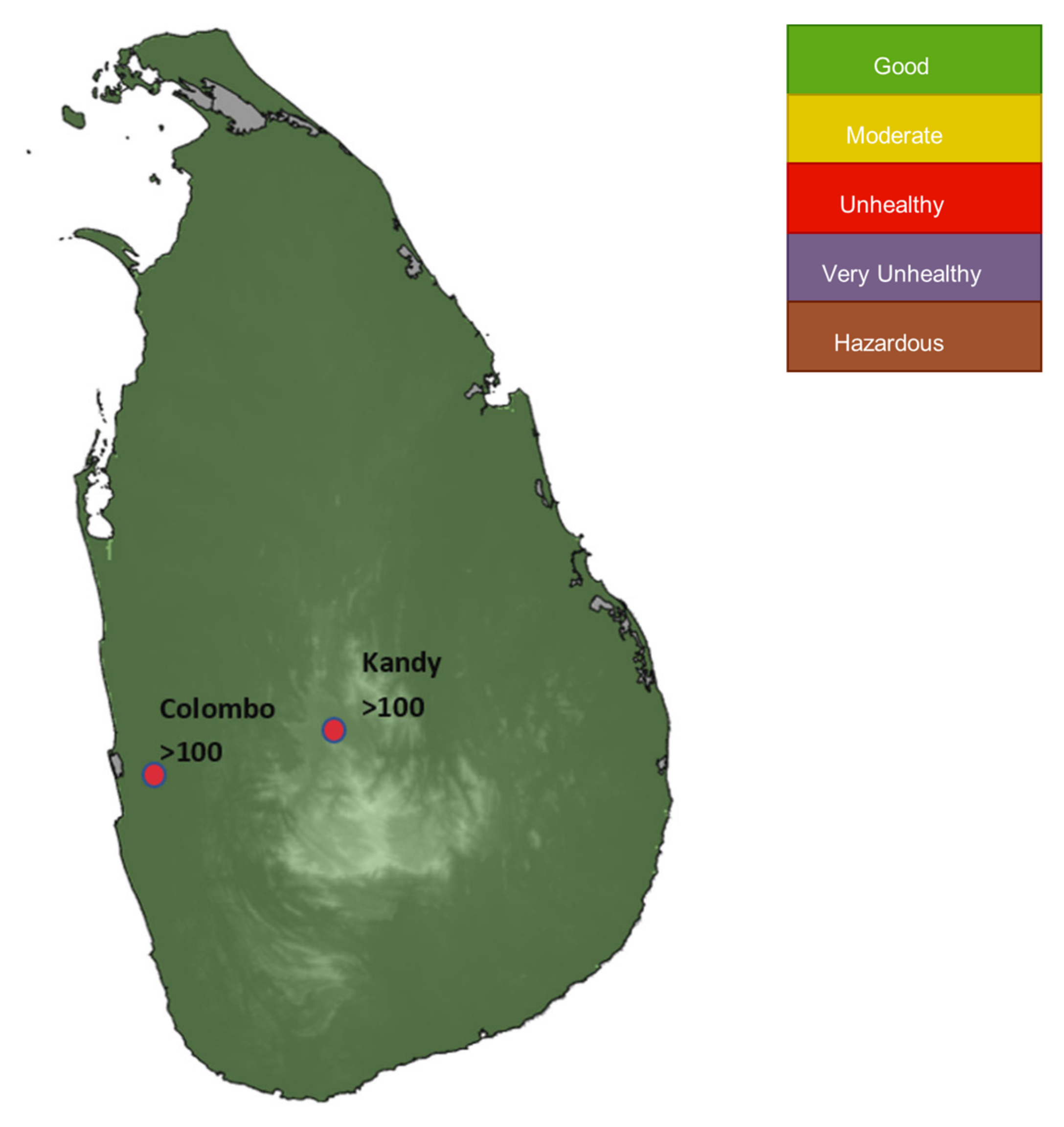
The World’s Air Pollution: Real-Time Air Quality Index clearly indicates the recent air pollution levels (as of March 2023) of the earth, which showcases that the air above Asian, African, and Latin American countries is not at a good level [
3,
4]. However, Asian countries are at a severe level as the majority of the world’s population lives in those countries. Importantly, PM
10 and PM
2.5 are at higher concentrations than what is given in WHO guidelines in most Asian countries. The situation is no different in Sri Lanka. The island has experienced some occasional severe air quality levels in 2022 and 2023 [
5]. This is mainly due to emissions from vehicles, the burning of organic materials, power generation, and petroleum refining. However, on average, most of the areas have had moderate air quality conditions in 2023. The Air Quality Index (AQI) was within the range of 51 to 100.
Figure 1 illustrates the air quality variation of Sri Lanka in 2023 based on the AQIs. Out of the 10 tested sites, 5 locations have been shown to be unhealthy for sensitive people’s levels of AQIs (AQI > 100).
As per the World’s Air Pollution: Real-Time Air Quality Index [
6] and
Figure 1, it can be identified that serious issues related to air quality are happening in many countries. Sri Lanka showcases a moderate air quality state in 2023, so precise forecasting of the PM
10 values for the future will lead to an increase in the quality of life by making decisions about air quality. The rate of urbanization is enhancing the air pollution levels in urban areas (considered highly urbanized areas such as Colombo, Jaffna, and Kandy [
5]. However, policy decisions are not strong enough to reduce them in developing countries. Sri Lanka has also faced this in cities like Colombo, Kandy, Jaffna, etc. Therefore, it is highly essential to forecast air quality levels in Countries like Sri Lanka. Therefore, this research paper for the first time in the context of Sri Lanka presents machine learning approaches to forecast air quality levels. This paper showcases some excellent approaches to forecast PM
10 levels in two of the most urbanized areas in Sri Lanka: Colombo, and Kandy. Moreover, in this research study, geographical properties such as altitude were considered while selecting Colombo (located in the Western Province, altitude 3.3 feet above sea level) and Kandy (Central Province, altitude 1640 feet above sea level).
2. Recent Work on Air Quality-Related Parameter Forecasting Using Soft Computing Techniques
Machine learning algorithms such as random forest (RF), linear regression (LR), and support vector regression (SVR) play an essential role as traditional algorithms for regression purposes. The functionality of the algorithms mainly depends on the dataset variations [
7]. Saikiran et al. [
7] conducted a study to predict air quality using machine learning algorithms using three algorithms, including RF, SVR, and LR. They achieved an RMSE value of 0.812 for RF as the highest functioning model for the specific dataset. In addition, Guo et al. [
8] conducted a study to predict air quality using a limited amount of data (23 July 2020 to 13 July 2021) for Shanxi, China’s meteorological station. The research study mainly focused on six parameters (SO
2, NO
2, PM
10, PM
2.5, O
3, and CO) in forecasting the AQI for a considered period range (8, 16, 24, 32, 40, and 48 h). As the functioning model, the researcher used an auto model network that could predict a functional capacity slightly above 50%. Importantly, the research team emphasized the model functionality with a comparative analysis [
8], using state-of-the-art algorithms for the comparative analysis to verify the functionality of the proposed auto model.
However, Popa et al. [
9] suggested that the optimized GPR algorithm outperforms other traditional algorithms, such as linear regression and SVM, in one of their research works carried out in Bucharest, Romania. Nevertheless, some other researchers stated that the hybrid deep learning models can function well in forecasting air quality data by competing with other traditional machine learning algorithms [
10,
11]. Therefore, it is well understood that algorithms can change their behavior based on the context of their usage, specifically with the location. Considering the comparative analysis, most of the research studies undertook this step to verify the proposed model [
8,
9,
10,
11,
12,
13,
14]. The functionality of the models differs due to the dataset variation and the gaps between the data. Researchers have worked on gathering hourly data to identify every simple variation in changes in air quality [
8,
9,
10,
11,
14]. The root mean squared error (RMSE), mean absolute error (MAE), mean squared error (MSE), mean absolute relative error (MARE), relative absolute error (RAE), and coefficient of determination (R
2) are some commonly used evaluating matrices to obtain a well-briefed evaluation on the models’ performance [
7,
8,
9,
10,
11,
12,
13,
14].
On the other hand, forecasting AQI and related data is an important process that requires precise output. Because of that, consideration of more factors that have the capability to affect air quality may lead to a more reliable result. Many previous studies [
7,
8,
9,
10,
11,
12,
13,
14] have elaborated on the effect of considering such data on the final output of the models. It has been identified that most of the research studies considered CO, NO
2, O
3, SO
2, PM
2.5, and PM
10 as their input parameters because of their importance.
3. Materials and Methods
3.1. Study Area and the Dataset
According to the statistical data representation of the Sri Lankan air quality parameters, it can be identified that with the time parameter, the severity of the negative effect is increasing gradually. As was stated above, two urban areas were considered for this research: Colombo and Kandy [
15]. Air quality data from the Battaramulla (in Colombo) (6.90103N:79.9265E) and Kandy (7.29262N:80.63564E) air quality-monitoring stations (AQMS) are managed by the Air Resource Management and Monitoring Unit (ARM&M Unit), Central Environmental Authority, Sri Lanka.
Figure 2 showcases these two monitoring locations.
Kandy is in central Sri Lanka, with an average height of 500 m from sea level, whereas Battaramulla is just located 11 m above sea level. In addition, Kandy has a lower population density and a lesser amount of industrial activity compared to the Battaramulla area. Therefore, the air quality levels can be expected to have two different compositions. Hourly data for 12 variables, including ambient temperature (AT), relative humidity (RH), solar radiation (SR), rainfall (RFL), wind speed (WS), wind direction (WD), O3 concentration, CO concentration, NO2 concentration, SO2 concentration, PM2.5, and PM10, were obtained from 1 January 2019 to 31 May 2021. Therefore, the dataset includes seasonal changes and their effect on air quality.
These parameters are highly important in determining air quality in the atmosphere. The absolute temperature increment affects the rate of harmful ozone creation [
17]. Higher and lower relative humidity significantly impacts the air quality because it creates a favorable environment for microscopic living beings to spread. Moreover, high RH may lead to a foggy environment. In addition, solar radiation directly impacts the temperature of the environment. Therefore, the combination of these meteorological parameters can impact the generation rate of toxic substances [
18]. Wind speed and direction are factors that have the ability to increase air quality by dispersing air pollutants. Areas with high wind speeds have lower amounts of contaminants [
19]. Therefore, they impact the PM
10 and PM
2.5 levels in the atmosphere. On the other hand, O
3 concentration affects lung functionality and directly impacts the ecosystem [
20] with SO
2 [
21], CO concentration reduces the oxygen level in the blood, and NO
2 concentration helps with the formation of acid rain. PM
2.5 and PM
10 are particles less than 2.5 µm and 10 µm in diameter. They have a direct impact on climate change and human health [
22].
Figure 3 showcases the data variation of a few selected parameters for Battaramulla and Kandy for the considered period before cleaning them.
Figure 3a–c clearly presents the higher levels of SO
2, PM
2.5, and PM
10 values for Battaramulla throughout the considered period. It can be clearly seen that the Kandy area had much better air quality than can be seen in Battaramulla considering the illustrated three parameters. Seasonal variations can also be visualized from these plots (
Figure 3), in addition to the impact of COVID-19. Some months were under lockdown conditions due to COVID-19, and the air quality was significantly enhanced during those days.
Battramulla had the highest PM
2.5 level of 140 µg/m
3 and the highest PM
10 level of 200 µg/m
3. Similarly, Kandy had the highest levels of PM
2.5 and PM
10 at 115 µg/m
3 and 190 µg/m
3 (refer to
Figure 3a–f—average daily data). This could be due to high levels of construction dust in both cities. Even though it was during the COVID-19 pandemic period, there was some heavy construction going on in both cities. However, these sites were not covered properly as per the standards. Thus, the construction dust particles can be clearly visualized. The Sri Lankan government has made a policy decision to move most of the administrative buildings from greater Colombo to the Battaramulla area, and the construction will continue for a few years. Similar construction projects can be seen in Kandy for rebuilding the congested city.
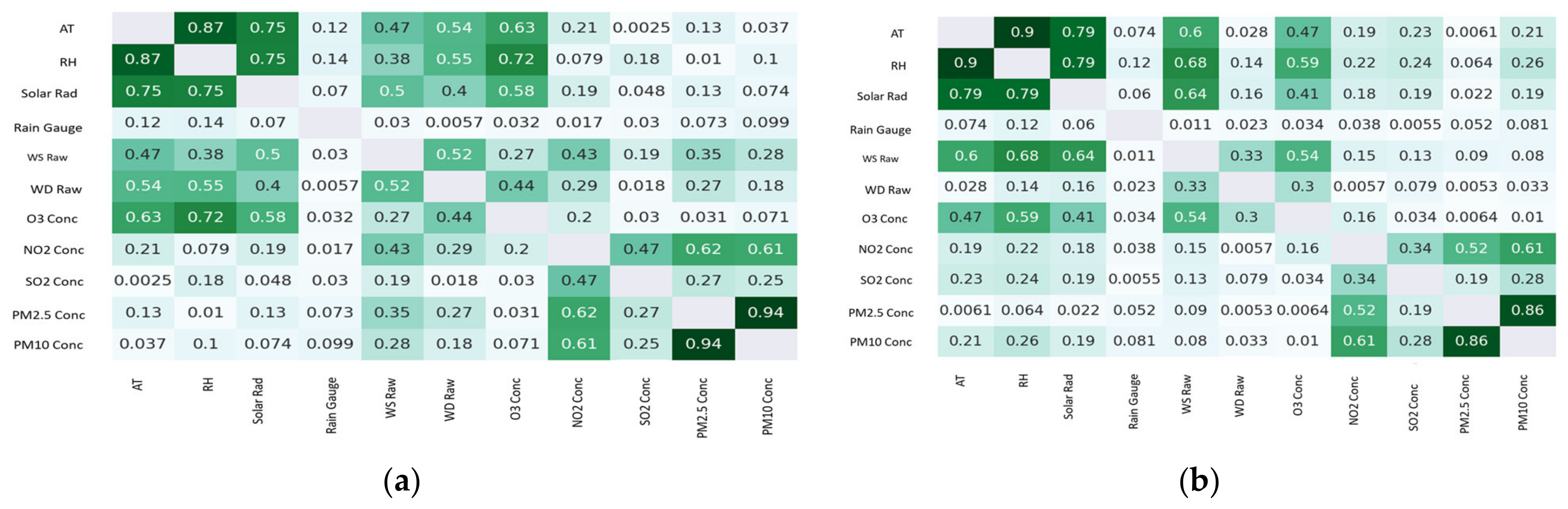
Figure 4 showcases the Pearson coefficients of correlation between each parameter for the two locations. It can be clearly seen that PM
2.5 and PM
10 had higher correlation coefficients. In addition, similar higher correlation coefficients can be seen for relative humidity and temperature.
3.2. Mathematical Formulations (Defining the Algorithms)
This section describes the mathematical functions of the algorithms, including XGBoost, CatBoost, Light BGM, LSTM, and GRU, that were used in the analysis.
3.2.1. XGBoost Algorithm
XGBoost is an algorithm that follows the ensemble approach with a switch to the decision tree model. The ensemble model is a combination of low-performance models to yield accurate results. At the end of the ensemble model, the final output is through another final model. It follows gradient boosting for the optimization of the algorithm [
7]. Moreover, XGBoost provides many advantages compared to other algorithms, such as high-speed performance. The reason behind this high-speed performance is parallel functioning, regularization, and treating the missing values in the dataset.
Considering the dataset as
, this dataset is a dataset with
number of samples and
number of features. Therefore, let the value predicted by the model be
.
denotes the independent regression tree, whereas
denotes the
ith sample of the
tree prediction score achieved.
Considering Equation (1) [
23], with the above-mentioned parameter definitions, can illustrate the objective function of the models as follows.
denotes the loss, which is calculated as the difference that arises between the predicted
and the real
. Moreover,
represents the complexity of the model, which handles the model’s overfitting [
23,
24]. It can be identified that the XGBoost can work very efficiently compared to other state-of-the-art models.
3.2.2. CatBoost Algorithm
CatBoost is an algorithm composed of the gradient-boosting decision tree and the categorical features. Because of such a background, it can be identified as a developed model of the gradient-boosting decision tree (initially, this follows the theories of the decision tree). Since boosting is used to develop the CatBoost algorithm, it uses some weak models as the combined model for the prediction, as in XGBoost. CatBoost can function well under classification, regression, and forecasting. The most common advantages of the CatBoost algorithm are that it can process categorical features, overcome the need for data preprocessing, and support the missing values of the dataset [
25].
The prior value of the random permutation is applied with the use of the random permutation by making the permutation
. Let P be the prior value and w be the weight value corresponding to the value of P [
26].
is represented by Equation (3) [
26].
Considering the same dataset as explained with XGBoost, it can be illustrated as .
3.2.3. LightBGM Algorithm
LightBGM is an algorithm developed by using the GBDT background. The main achievement of this algorithm is that it can perform well by enhancing memory utilization. Considered XGBoost, LightBGM uses a histogram-based, highly optimized decision-making algorithm [
27]. This method improves the computational memory’s efficiency and optimal functioning. Mainly, the LightBGM has the functionality of reducing the error on the predicted value and the test value, noting the expected results as
The model development undergoes
number of decision trees.
Equation (4) [
27] represents the objective function of the gradient-boosting algorithm. The loss function of the above equation is represented by F, whereas the regularization factor is denoted by
. The decision tree improvement with the
value is denoted with
as in Equation (5).
Undergoing the Taylor expansion for the loss function can be demonstrated in Equation (6) [
28], where
is the constant of the equation.
The optimization of the equation by removing the constant of the final objective function is denoted as follows [
28] in Equation (7).
The optimized object function in Equation (7) positively impacts the functionality of the model’s accuracy and efficiency.
3.2.4. LSTM (Long Short-Term Memory)
LSTM can be identified as a deep learning model that functions most likely as RNN. Difficult situations faced by the RNN can be covered using LSTM, such as long-term dependency problems, vanishing gradients, and exploding gradients. LSTM models are built using cells and gates. LSTM is based on three main functional areas, the forget gate (removes the irrelevant data), the input gate (updates with new information), and the output gate (releases the updated information as an output) [
29]. The mathematical equations used to build LSTM are one-time step equations, where each equation needs recomputing after one iteration to yield the results (refer to Equation (8)).
denotes the weight matrix used in LSTM, whereas
,
, and
represent the biased vectors of the model [
30]. The sigmoid activation function is represented by
. As for the three gates of LSTM,
represents the forget gate,
represents the input gate, and
represents the output gate.
represents the cell state. After the recompute is carried out, the new cell state is calculated by Equation (12) [
30].
Consider
as the projection matrix of the dimension reduction of
, where
represents the LSTM output [
30].
from Equation (13) [
30] represents the final model output of the LSTM model.
3.2.5. GRU (Gated Recurrent Unit)
GRU is a network capable of functioning well for the data of texts, speech, and time series data, which comes under the advancements in RNNs [
31]. Compared to LSTM, GRU shows similar functioning due to the use of the gate structure to send the information throughout the model. The gates used in GRU are the reset gate and the update gate [
32,
33]. The mathematical formulae for these two gates can be described in relation to Equations (11)–(13). The training time of GRU is low compared to LSTM, the reason being that GRU only uses hidden state
, as in Equation (13), and
is not calculated.
and
denote the update gate and the reset gate as vectors, respectively, based on Equations (14) and (15) [
34].
represents the sigmoid function, whereas the hyperbolic function is represented by
. The parameter matrix for the model is represented by
and
[
34].
3.3. Mathematical Formulation of Evaluation Matrices
Future decisions from the results of this research study can be extensively used for planning purposes. Therefore, justifying the accuracy of the developed model is highly essential. The following indices were used to assess the accuracy of the models. The mean squared error (MSE) is one of the simplest and most common evaluating matrices used in related studies. The predicted values and the actual values that were fed to the model are considered in the calculation of MSE (refer to Equation (17)).
where
denotes the actual values, whereas
denotes the predicted values. N denotes the number of samples selected from the dataset. According to Equation (17), the minimum value for the MSE means the model is getting better.
The mean absolute error (MAE) is the second index that was used in this study. The magnitude of the divergence between the true value and its prediction is referred to as the absolute error. The size of errors for the entire group is determined by the MAE by averaging the absolute errors for a set of forecasts and observations. The MAE is also known as the L1 loss function. The MAE supports the process of turning learning problems into optimization methods because it is one of the most widely utilized loss functions for regression situations. It also serves as a simple, quantifiable way to quantify errors in regression issues.
According to Equation (18),
denotes the actual values, whereas
denotes the predicted values. An MAE value closer to 0 represents higher accuracy of the model [
35]. The root mean squared error (RMSE) is another widely used index for accuracy [
7,
8]. The mathematical formulation for the RMSE can be seen in Equation (19).
The coefficient of determination (
) illustrates the percentage of the dependent variable’s variance that the independent variables account for collectively [
7,
8].
provides a straightforward 0–1 (0–100%) scale for evaluating the strength of the link between the developed model and the dependent variable. Equation (20) presents the mathematical formulation for
presents the mean value of the dataset. Higher values of
represent higher accuracy of the developed model. The mean absolute relative error (MARE) illustrates the mean absolute percentage difference between the test data and the precited data. Moreover, the MARE is a normalized metric and is relative (Equation (21)) [
36]. A lower MARE indicates better performance of the developed model.
The last index is the Nash–Sutcliffe efficiency (NSE). This evaluating matrix computes the ratio of the sum of squared residuals of the predicted values to the sum of squared deviations of the actual values from their mean.
Based on Equation (22), it is clear that values around 1 for the NSE represent higher performance of the model [
37].
3.4. Methodology
This research study set to forecast PM
10 values using the other air quality parameters for two urban areas: Battaramulla and Kandy (as shown in Equation (23)). As was stated earlier, both areas showcased higher concentration levels of PM
10. Therefore, the research focus was directed to forecast PM
10 levels. Five efficient forecasting algorithms described in
Section 4 were used for the forecasting purpose of this application, with the use of necessary libraries such as Keras and TensorFlow in a Python environment. In this research work, statistical models were considered over traditional deterministic models to identify the hidden interactions in the parameters considered and achieve an understanding of the complex patterns of the dataset. Moreover, with the availability of historical data and to be more flexible with the dataset (linear and non-linearity of the dataset), statistical models were considered over the deterministic models.
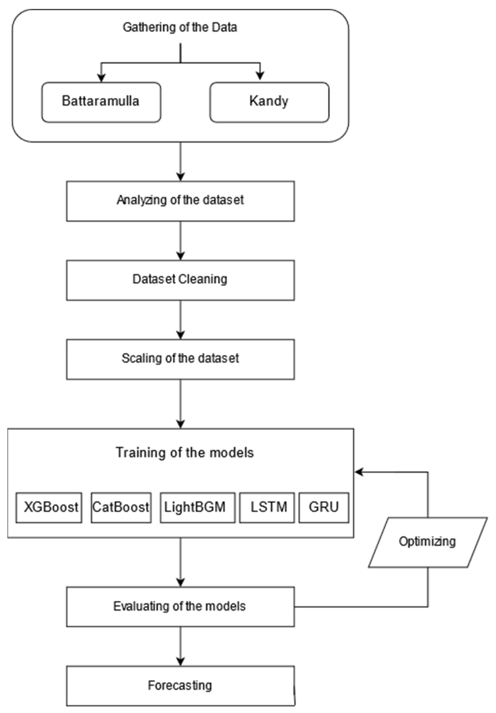
All five models were optimized based on the dataset used to obtain the maximum effectiveness of the models. The forecasting process was developed as given in the flowchart (refer to
Figure 5) considering several factors to achieve the maximum effectiveness of the dataset.
Figure 5 illustrates the process that followed to achieve the results mentioned in
Table 1 by forecasting air quality. Since manual optimization was used, the
Figure 6 describes the steps taken to achieve it.
One of the most critical steps of the proposed methodology is cleaning the dataset. Considering
Figure 3, it is possible to understand that there are gaps in the data between the considered period. It is due to the unavailability of the data in the collected dataset. Moreover, as a dataset-cleaning process, the rows with the missing values from the dataset were removed. After that, the dataset was restructured. It was identified that removing the data from the dataset did not impact the dataset’s pattern since all of the variables were cleaned. Initially, the datasets consisted of a total of 201,947 data points in the Kandy dataset and 195,123 data points in the Battaramulla dataset. After the cleaning process, the Kandy dataset was reduced to 114,996 data points and the Battaramulla dataset was reduced to 100,380 data points. In the format of time and date, the Kandy dataset was reduced to 10:00 a.m. on 1 January 2021 and the Battaramulla dataset to 12:00 a.m. on 8 October 2020. Normalization is a step that positively impacts the overall model functionality. Since the dataset followed a pattern due to seasonal changes, the normalization normalized the dataset to make it easy to understand by the model. A MinMax scaler was used to achieve this target. For the feeding of the datasets to the models, the data were divided into training and testing as follows:
Kandy: training = (6988, 12), testing = (1631, 1);
Battaramulla: training = (5970, 12), testing = (1488, 1).
To prevent the models from being overfitted or underfitted, the following approaches were separately carried out with all five models. For XGBoost, the regularization parameters
(L2 regularization) and
(L1 regularization) were optimized as
= 0.8 and
= 0.9. In CatBoost, L2 regularization was carried out by setting the value to 3 to overcome overfitting without leading to underfitting. In the use of LightBGM,
and
values for the optimization were used to avoid overfitting by assigning the values as 0.7 for both parameters. In LSTM, early stopping and dropout were used to stop overfitting. Moreover, batch normalization was used in LSTM. Similar to LSTM, GRU was also optimized by using early stopping, dropout, and batch normalization to stop overfitting.
Figure 6 represents the stepwise explanation of the approach used in order to forecast through continuous optimization of the models. Moreover, to find the best hyperparameters for the models, manual tunning was used for XGBoost, CatBoost, GRU, and LightBGM. With a proper investigation of the models’ results, manual tuning was carried out. Moreover, in the LSTM network, a grid search technique was used to identify the best matching hyperparameters. With the optimization of the hyperparameters manually and with the grid search, higher performance of the models was achieved for this study.
As explained earlier, five algorithms were used to conduct the forecasting process. The performance of all models was evaluated using following evaluation parameters (refer
Table 1). The model training, evaluating, and forecasting processes were carried out using the same number of computational resources to avoid the negative impact that could happen due to the resources used. A personal computer with 2 CPU cores, 12 GB RAM, and Nvidia K80 GPU with GPU RAM of 12 GB was used for this analysis.
4. Results and Discussion
This research study focused on forecasting the PM
10 value for the future starting from June 2021. According to
Figure 3c,f, it can be identified that PM
10 made a high impact and a variation in the air quality in both areas. The peak value of PM
10 reached a peak of around 200 µg/m
3. Therefore, these levels significantly impact human health. This is also verified by the number of patients hospitalized (Kandy National Hospital and Peradeniya Teaching Hospital) due to respiratory-related diseases [
38].
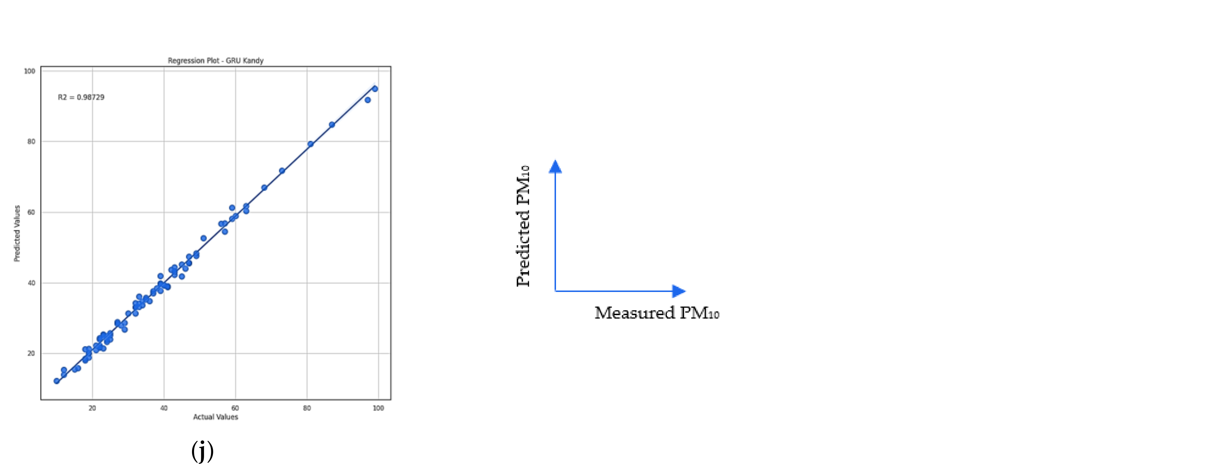
Figure 7 presents the coefficient of determination for predicted vs. measured PM
10 levels under five algorithms for both Battaramulla and Kandy. They all showcased a very high forecasting efficiency based on the higher R
2 values (which were almost 1). Moreover,
Figure 7a represents a small deviation, as a score of
was achieved. However, it is clear that all five models applied worked very well on the two datasets.
Figure 8 presents some of the predicted PM
10 variations against the measured PM
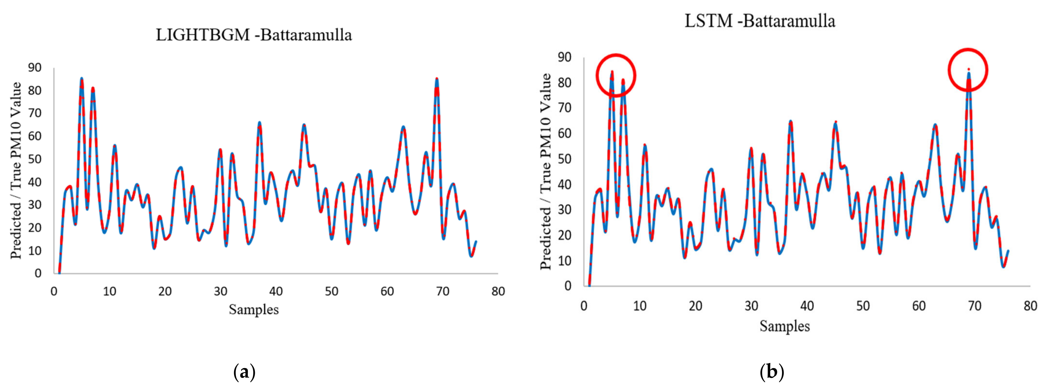
10 values for selected algorithms (highest performance and lowest performance) for both urban areas. Some disputes can be observed for the XGBoost algorithm (circled in red), whereas LightBGM produced excellent overlap for the measured data. The hyperparameter tuning was carried out using the manual optimization of the hyperparameters in the XGBoost algorithm. The manual search was carried out by following a few peak values of the evaluating parameters and optimization around those points. Moreover, a few disputes can also be seen for other tested algorithms (which are not shown here due to extended length). Nevertheless, LightBGM had the highest efficiency in predicting peak values.
Table 1 represents all the results obtained throughout this application to identify the best-performing model for the considered locations. Overall, the results demonstrate that all the models functioned well for both locations. Moreover, this table helps to obtain a numerical comparison of the model performance considering six evaluating matrices. This will lead to identifying the best performing algorithms with the supplied computational power.
Moreover, LightBGM was the best functioning algorithm for predicting the data for Kandy. It achieved an value of 0.9999. Moreover, when it comes to real-world application, 0.9999 is an outstanding value. Even though both LightBGM and CatBoost achieved likely similar results to the MAE and the RMSE, it can be identified that LightBGM performed better than CatBoost in predicting the PM10 values.
The results gained for the Battaramulla area demonstrate that all models achieved the best prediction scores. Considering all evaluating matrices, it can be identified that LightBGM was the best-performing algorithm in predicting PM
10. LSTM was the lowest-performing algorithm in the Battaramulla location compared to the other considered algorithm models. Therefore, it can be verified that LightBGM had the functionality to predict the actual testing values accurately for PM
10 for both the locations: Battaramulla and Kandy. Referring to
Figure 7 and
Table 1, it is evident that all the models achieved a considerably higher result in this research study. The main background behind that scenario is the continuous optimization of the algorithms to achieve the best results without leading to overfitting and underfitting. The dataset was composed of low noisy data and underwent visible seasonal changes. Moreover, the identifiable data variations also made a direct impact on the higher results of this research activity.
Therefore, the forecasting process was carried out using these algorithms as identified for the Battaramulla and Kandy urban areas for the next three months.
Figure 9 summarizes the forecasted PM
10 values. It represents how the PM
10 could be changed for the next three months starting from October 2020 for Battaramulla and from April 2021 for Kandy based on the availability of data. To identify the variation, the previous month’s data were plotted. Moreover, the data show that the forecasted data also followed the same pattern. Additionally, it demonstrates that, following the same pattern with the seasonal variation, there was a slight increase in the peak values.
With the continuous analysis of time series data for PM10 values for both locations, it was possible to predict the quality of life that humans can carry out in the respective areas. Air is a main factor that contributes to the existence of human beings. In the contribution to the well-being of human life quality, it is possible to recognize that PM10 value forecasting is a factor that helps the world population live a healthy life.
From a biological point of view of the effect of PM
10, the research carried out by the International Agency for Research on Cancer (IARC) has demonstrated that long-term exposure to PM
10 in the air may cause respiratory illnesses such as lung cancer. Moreover, other severe cases recently identified include wheezing, asthma, high blood pressure, bronchitis, strokes, and heart attacks. The most severe case is premature death. More information on health-related issues can be found in Lu et al. [
39]. Therefore, it is essential to forecast the PM
10 level. This helps ensure a safer environment for the people living in a certain area.
5. Conclusions
This research study was carried out to forecast the PM10 values for the selected areas of Sri Lanka: Battaramulla and Kandy. The five tested algorithms showcased higher performance in forecasting PM10 values for both Battaramulla and Kandy. Out of the tested algorithms, the LightBGM algorithm was excellent for the Battaramulla dataset, and the same LightBGM algorithm was the best for Kandy. The forecasted PM10 for 3 months followed the same patterns that were observed in the measured dataset. Therefore, the developed forecasting models can effectively be used for planning activities in the cities of industrialized Battaramulla and religious Kandy.
It was identified that the proper optimization of algorithms led to producing excellent results from the prediction models. In addition, the datasets might have had lower noises while representing seasonal behavior. Alyousifi et al. [
40] suggested that their hybrid fuzzy model has excellent performance, especially for nonseasonal variables. However, the model developed in this research efficiently captured the seasonal behavior of datasets. Therefore, this information can be shared with the public in real time using telecommunication networks for any necessary precautions.
Since air quality is a primary factor affecting human health and the complete functionality of the environment, forecasting the factors that increase the negative impact on air quality is very important. It is also important to forecast the air quality index (AQI) for all of Sri Lanka using the method adopted herein. However, available data shortages would be a major limitation in the Sri Lankan context. Forecasting algorithms on microcomputers with the necessary sensors can be a future direction for urbanized cities to showcase the forecasted air quality levels. When adverse air quality levels are forecasted, higher-risk people can be given some warning.

 ,
, 


