Article

The Use of Satellite Synthetic Aperture Radar Imagery to Assist in the Monitoring of the Time Evolution of Challenging Coastal Environments: A Case Study of the Basilicata Coast

by
Emanuele Ferrentino
1,
Nicola Angelo Famiglietti
2,*,
Ferdinando Nunziata
3,
Giovanna Inserra
3,
Andrea Buono
3,
Raffaele Moschillo
2,
Antonino Memmolo
2,
Gerardo Colangelo
4,
Annamaria Vicari
2 and
Maurizio Migliaccio
1,3
1
Istituto Nazionale di Geofisica e Vulcanologia (INGV), 00143 Rome, Italy
2
Istituto Nazionale di Geofisica e Vulcanologia (INGV), Sezione Irpinia, 83035 Grottaminarda, Italy
3
Dipartimento di Ingegneria, Università degli Studi di Napoli Parthenope, 80143 Napoli, Italy
4
Direzione Generale dell’Ambiente del Territorio e dell’Energia, Regione Basilicata, 85100 Potenza, Italy
*
Author to whom correspondence should be addressed.
Environments 2023, 10(12), 212; https://doi.org/10.3390/environments10120212
Submission received: 18 September 2023 / Revised: 6 November 2023 / Accepted: 1 December 2023 / Published: 3 December 2023

Abstract

:
This study focuses on a very complex environment, namely the Ionian coast of the Basilicata region, Southern Italy, which includes different kinds of beaches, river mouths and built-up areas. This complex environment is used as a test case to analyze the time variability of the coastline using measurements that were remotely sensed by the satellite European Copernicus Synthetic Aperture Radar (SAR) mission. First, the accuracy of the coastline, extracted by the SAR, is discussed with respect to finer-spatial-resolution drone-based light detection and ranging (LIDAR) measurements. Then, a time series of SAR dual-polarimetric measurements acquired by the European Copernicus mission is used to discuss the time variability of the coastline of the area of interest in a time period spanning from 2015 to 2021. The experimental results show that the accuracy of the SAR-based coastline is better than 15 m, which is reasonably good precision for monitoring the erosion/accretion processes that characterize the area of interest at a moderate scale. The estimated time variability of the extracted coastline suggests a dominant erosion process, which is always within 60 m.

1. Introduction

Coastal regions represent areas where most of the population lives, where most economic activities take place and where most of the land–sea interactions occur. The effective monitoring of coastal areas is of crucial importance to observe processes due to both anthropomorphic activities (e.g., mining of seashore sand for building purposes) and natural phenomena such as coastal erosion, which threaten the stability of land and the safety of people living along the coasts. Moreover, the increasing effects of climate change could be devastating to vulnerable coastal and marine areas as well as to the function and structure of their ecosystems. For instance, sea level rises change the shape of coastlines, contributing to coastal erosion [1].
In this study, we focus on the Ionian coast of the Basilicata region in Southern Italy, which is a significant heritage landscape of socio-economic value that is subjected to natural and human-made processes affecting the sustainable development of the region. Among these processes, coastal erosion has severely affected the Ionian coast, leading to the disappearance of large beach areas and parts of the cordons of coastal dunes. The severe storms that hit the Ionian coast confirmed the extreme vulnerability of this area to erosion phenomena. In recent years, several storms caused a further retreat of the shoreline and severe structural damages as well as secondary effects related to the pollution of freshwater aquifers at the service of an area of a large agricultural region.
The studies carried out in recent years dealt with the implementation of mitigation countermeasures that only partially mitigated the effects of the subsequent hazard events, such as those that occurred in 2011 and 2013. The evolution of the Basilicata coast is also significantly affected by the transport of sediments due to rivers and currents originating from the Gulf of Taranto. The contributions of sediments by the rivers of Basilicata vary from gravel–pebble sediments in the Sinni River to sandy–silty sediments in the areas surrounding the Basento–Bradano River. Consequently, the sea energy has a greater erosive effect on fine sediments and a lower effect on coarse sediments, causing differential erosion phenomena. By analyzing relevant studies in the literature on the geomorphological data related to the evolution of the Basilicata coast, we can also note periods calling for an accretion of the coastline [2]. This underlines the fragile balance between anthropomorphic activities involving coastal areas and their geo-environmental sustainability.
In recent decades, the lack of solid transport of waterways of the Basilicata region determined, with particular importance along the Ionian coast, a crisis of the coastal feeding system that affected the balances that regulate coastal dynamics. The main cause of the lack of solid contribution of the Lucania rivers was likely related to the construction of reservoirs for irrigation, industrial or electricity supply, which affected all rivers between 1955 and 1994 with the exception of the Cavone river. The contribution of sediments was further reduced by the collection of aggregates along the riverbeds and by the hydraulic works carried out during this period. Among the most significant effects of the modified balance of coastal dynamics along the Ionian belt, the most evident one was a significant retreat of the coastline along large stretches of the Ionian coast, which caused severe damage and limited economic activities.
Within this context, remote sensing sensors play a very important role. The availability of satellite-derived coastal imagery significantly changed the way coastal data are collected, providing daily to weekly surveys of thousands of kilometers of coastline. Optical data are widely employed for coastal monitoring [3,4,5]. However, the operational use of optical satellite measurements is limited to daylight and cloud-free conditions due to its dependence on sun and favorable weather conditions.
To overcome these limitations, a key remote sensing instrument for coastline monitoring is Synthetic Aperture Radar (SAR) due to its all-day and almost all-weather imaging capabilities together with its wide area of coverage. Most of the coastline extraction studies in the literature are based on image processing techniques and edge detection algorithms applied to single-polarization multi-looked SAR images, and, typically, the extracted coastal profile is then contrasted with the coastline that is visually inspected from collocated optical imagery [6,7]. In [8], the coastline extraction from the SAR data is performed using wavelet and active contour methods, while a new approach is proposed in [9] to improve the accuracy and efficiency of coastline detection based on the gradient vector flow snake model. The coastal extraction problem from SAR data can also be addressed according to a statistical estimation framework, in particular, exploiting the Bayesian estimation theory [10]. In addition, the advent of new SAR technologies equipped with high-performance polarimetric modes triggered the development of value-added products in several thematic domains including coastal areas. Multi-polarized SAR imagery has been exploited for coastal area observation purposes in [11,12], where the coastal extraction is addressed using image anisotropic diffusion and spectral–textural segmentation. The accuracy of the coastline extraction process, which is assessed using a reference coastline that is manually extracted from the SAR images, depends on the SAR incidence angle frequency and polarization. In [13], the cross-polarization channel is shown to provide the best performance at lower incidence angles (i.e., <30°), while no polarization dependence is observed at larger incidence angles (i.e., >30°). In [14,15], it is shown that higher frequencies (C- and X-band) perform best. In [16,17,18], the coastline extracted using polarimetric SAR imagery is contrasted with ground-based information obtained using global positioning system (GPS) measurements. The SAR data set consists of X-band dual-polarimetric Ping Pong (HH + VV) COSMO-SkyMed SAR imagery collected in the muddy sand intertidal flat area of Lingang New City, China [16]. The accuracy of the extraction process is focused to be lower than 4 pixels. In [17], multipolarization C- and X-band SAR imagery collected over Monasterace, Italy are used to extract the coastline with an accuracy that is lower than 5 pixels. In [18], full-polarimetric C-band RadarSAT-2 SAR images are used for coastal area observation purposes. The coastline extracted from the SAR data set using full-polarimetric channels is shown to be around 4 pixels. In all of the above-mentioned studies, the speckle noise that affects the SAR imagery was filtered using conventional local approaches. Recently, different approaches based on non-local filters have been exploited to reduce speckle noise in SAR imagery while preserving the fine spatial details. The use of non-local speckle filters for coastline extraction purposes is addressed in [19], where single-polarization X-band TanDEM-X pursuit monostatic SAR measurements were considered. In [20], the “twin-problem” related to the extraction of the waterline associated with a reservoir is addressed using dual-polarimetric SAR measurements with the main goal of estimating the waterbody area. The accuracy of the estimated waterbody area is contrasted with estimates obtained using single-polarization SAR measurements and with ancillary in situ observation.
The state-of-the-art analysis points out that the accuracy of the coastline extracted from the SAR imagery is addressed either by using point-wise GPS information or by contrasting the SAR-based coastline with the one extracted from the imagery that was remotely sensed using optical instruments. The first option provides very precise (but expensive and time-consuming) accuracy estimations that refer to a specific scenario and cannot be straightforwardly generalized. The second approach is adopted in most cases, but it is intrinsically less precise since it relies on the comparison of coastlines extracted from different remotely sensed measurements collected at different spatial resolutions and imaging geometries.
In this study, a twofold objective is pursued: (a) discussing the accuracy of the coastline extracted by SAR imagery using very accurate drone-based measurements obtained by jointly exploiting LIDAR and orthorectified photos, and (b) discussing the time evolution of the coastline extracted using a time series of SAR imagery. To reach these goals, an area of interest is selected that belongs to the Ionian coast of the Basilicata region, Southern Italy; see Figure 1. This coastal area, as previously discussed, is a very challenging environment since it includes sandy beaches, river mouths, built-up areas, etc., on one side, and it has been affected by both erosion and accretion phenomena on the other side. Hence, the selected test case calls for a morphology that is heterogeneous enough to test the accuracy of the SAR-based coastline under different conditions, and it calls for a significant time variability that is worth observing using satellite SAR measurements.
The remainder of the paper is organized as follows: in Section 2, after a brief review of SAR polarimetry, the rationale of the proposed approach is discussed in detail. The test site, dataset and experiments are described in Section 3 and Section 4, while the conclusions are drawn in Section 5.

2. Methodologies

This section describes the methodology that underpins the extraction of coastline using SAR and LIDAR measurements.

2.1. Processing of SAR Measurements

The proposed processing chain, depicted in Figure 2, ingests dual-polarimetric (DP) SAR measurements, i.e., the standard acquisition mode of the European Copernicus Sentinel-1 SAR mission over coastal areas. Those measurements consist of the scattering amplitude associated with co- and cross-polarized channels, i.e., Sxx and Sxy, with x, y standing for the linear horizontal (h) and vertical (v) polarization basis. The following steps are implemented:
  • Pre-processing: This includes polarimetric calibration, multi-looking to reduce the speckle noise using an N × N boxcar window and geo-coding. In this study, N = 9 is used since it represents a good compromise between speckle reduction and preservation of spatial details.
  • Feature extraction: This is a key step in coastline extraction that relies on the enhancement of the land/sea contrast. This is very important to make the subsequent steps more robust and effective. This means that a metric that increases land/sea separation in a broad range of sea state conditions and incidence angles is to be selected. In this study, the combination of co- and cross-polarized scattering amplitudes is selected:
r = ⟨|Sxx||Sxy|⟩
This metric has been shown in [17] to increase the land/sea contrast under most sea state conditions and under different land types; therefore, it is used here as a preliminary step to facilitate the generation of a binary map that distinguishes land from sea.
According to the metric r, low values are expected over the sea surface due to negligible cross-polarized backscattering, while larger r values are expected over land—according to coastal morphology, e.g., sand, rocks, vegetation, urban, ice, etc.—due to the significant contribution of both co- and cross-polarized backscattering.
  • Binary image generation: A binary image, i.e., an image where land and sea are distinguished, is generated using a constant false alarm rate (CFAR) global threshold method [21]. The CFAR algorithm separates land from sea pixels according to the decision rule that consists of comparing r with a threshold. In this study, the statistical distribution of r over a clutter area, i.e., an area belonging to the sea surface, is found to be well approximated by a Burr probability density function (pdf); hence, the threshold η can be set as a function of the probability of a false alarm Pfa using the following formula:
P f a = t h α β α μ r μ 1   β + r μ α + 1 d r   ,   r >   0 ,   η = β P f a 1 α 1 1 μ
where α and μ are the non-negative shape parameters, while β is the non-negative scale parameter of the Burr distribution. In this test case, a Pfa equal to 10−6 is used.
  • Post-processing: This consists of polishing the binary image by removing artifacts and holes using a morphological filter.
  • Edge detection: This consists of extracting the 1-pixel continuous coastline by processing the binary image; here, this is carried out using a well-known edge detector, Sobel kernel, which measures the 2D spatial gradient on the binary image to emphasize edges. This Kernel provides the best trade-off between detection accuracy and time effectiveness.

2.2. Processing of LIDAR Measurements
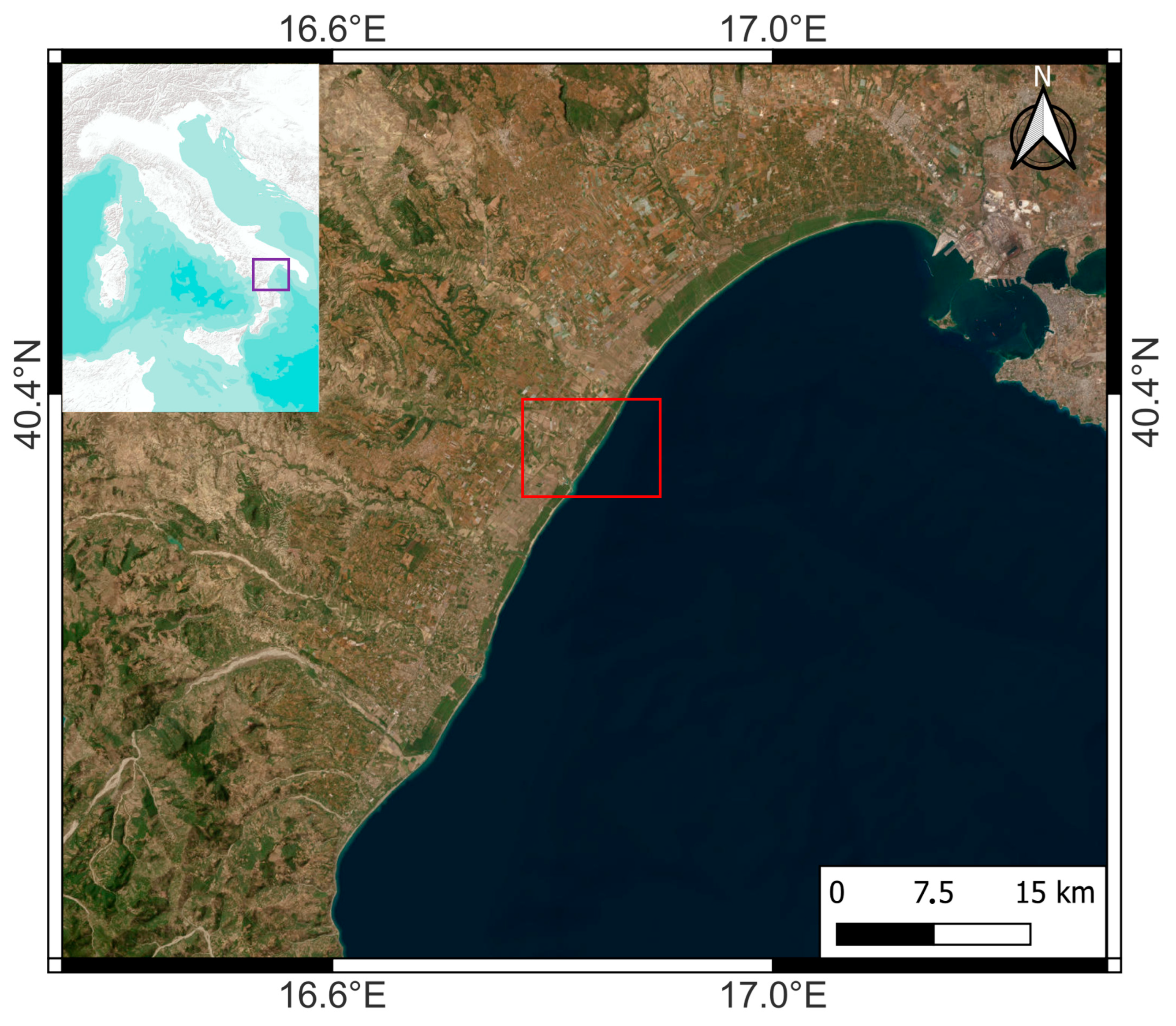
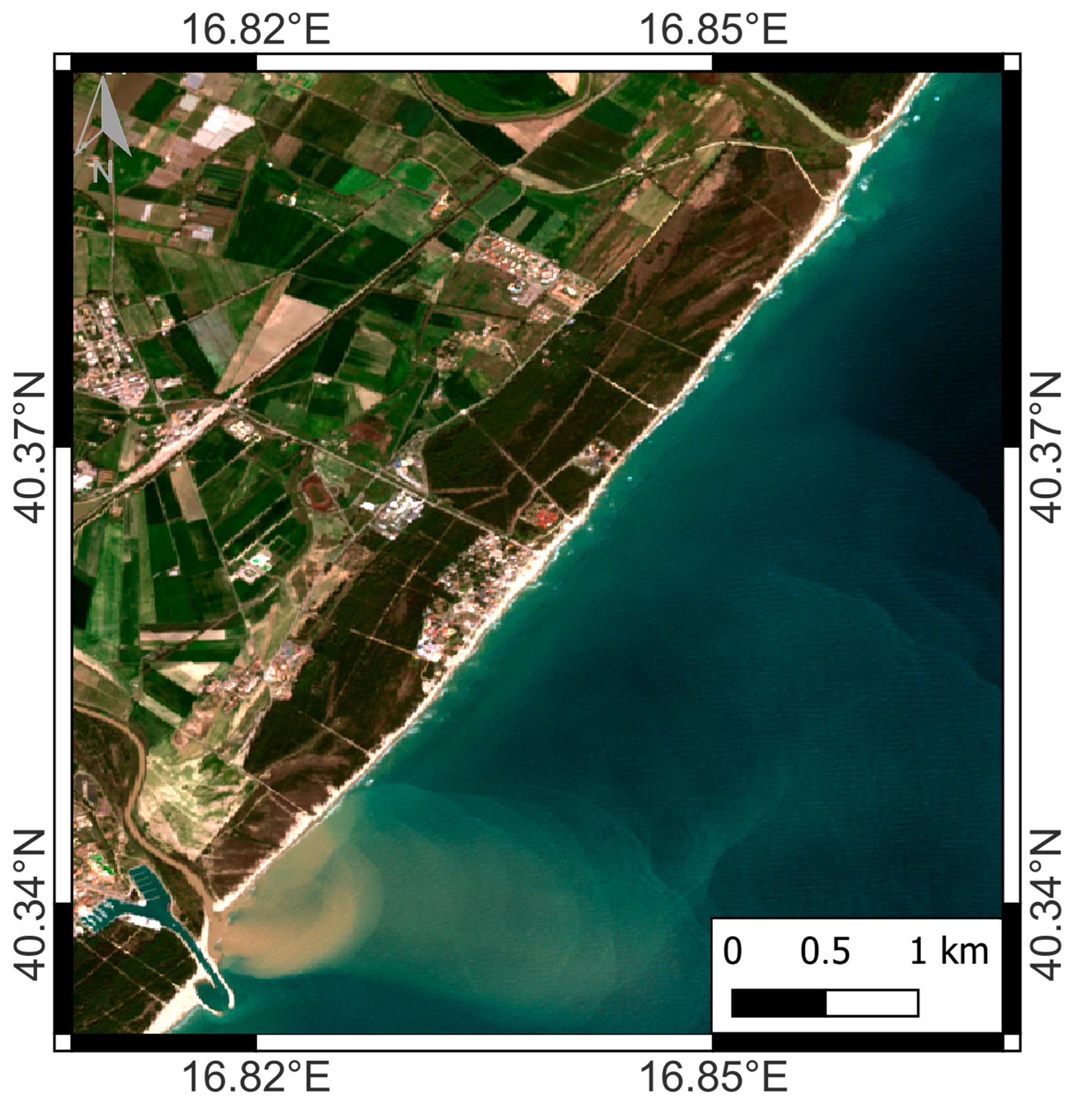
The LIDAR processing consists of the extraction of the coastline from the LIDAR measurements [22,23,24,25].
The raw data collected by the LIDAR system are processed with GNSS differential corrections and further refined with the IMU corrections to provide a 3D point cloud. The methodology used to extract the coastline from the pre-processed LIDAR measurements consists of generating the digital surface model (DSM) and contour lines with a spacing of 10 cm. The coastline is extracted using the 0 m (a.s.l.) level curve and refined using the orthorectified photos spatially and timely collocated with the LIDAR measurements.

3. Data Set

The data set consists of Sentinel-1 C-band dual-polarimetric VV + VH interferometric wide (IW) SAR ground range detected (GRD) scenes and LIDAR measurements; see Table 1.
The area of interest includes 40 km of the Basilicata Ionian coast, southern Italy; see Figure 3, in which a Sentinel-2 MSI true color image is shown for reference purposes. The area of interest includes the Metaponto Plain, which extends from the low hills of Matera to the Ionian Sea and is characterized by beaches of fine golden sand, and the Pollino National Park, characterized by wide beaches of sand and pebbles.
The SAR data set consists of 28 SAR scenes collected under a descending pass over the Basilicata coast from 2015 to 2021. The spatial resolution is 10 m × 10 m (range × azimuth), and the angle of incidence (AoI) is 41°; see Table 1.
The LIDAR measurements were collected on 12 April 2022 over the area of interest (see Figure 3). The LIDAR acquisition is collocated with the Sentinel-1 SAR scene collected on 12 April 2022 at 16:48 UTC. The LIDAR uses a near-infrared (NIR) laser centered at 905 nm and it is equipped with a compact point cloud data acquisition system (Gs-100C+ by Geosun, https://www.geosunlidar.com), which uses a new-generation Livox Avia laser scanner (https://www.livoxtech.com), an integrated positioning system (GNSS and inertial measurement unit (IMU)) to determine the position of the drone and a 26-megapixel optical camera used to color (RGB) the point cloud. The LIDAR sensor acquires 240,000 points/second in Single Echo mode and 720,000 points/second in Triple Echo mode, with a measurement accuracy of less than 10 cm (110 m above ground level). It provides a 70° circular field-of-view (Fov). The laser unit, a 905 nm Class1 (IEC 60825-1:2014) laser, achieves a range accuracy of about 2 cm. This tool was operated on board a DJI M600 pro (https://www.dji.com) hexacopter (with a maximum payload of 6 kg), which also includes a flight control system (DJI A3 Pro) with triple modular redundancy based on diagnostic algorithms that compare and use data from three GNSS systems.
The LIDAR measurements are collected over the area of interest according to seven flight paths that are annotated in the Google Earth image shown in Figure 4. The red and green arrows indicate the drone take-off and landing points, respectively, while the zoomed-in version of the paths is annotated in the seven boxes. The drone flew at an 80 m altitude (AGL), and the maximum distance from each take-off location was 500 m. The green lines stand for the flight line, while the yellow horizontal line stands for its ground projection. The yellow vertical lines stand for the intermediate waypoints. The LIDAR measurements are then geocoded by correcting the UAS GNSS data in Post Processing Kinematic (PPK), using, as a basis, the Craco station (CRAC) of the INGV permanent GNSS network (https://doi.org/10.13127/ring) [26].

4. Experiments and Results

In this section, first, the accuracy of the coastline extracted using the SAR measurements is discussed against the coastline extracted by the drone-based LIDAR measurements. Then, the time variability of the coastline belonging to the area of interest is discussed by using the whole time series of SAR scenes.

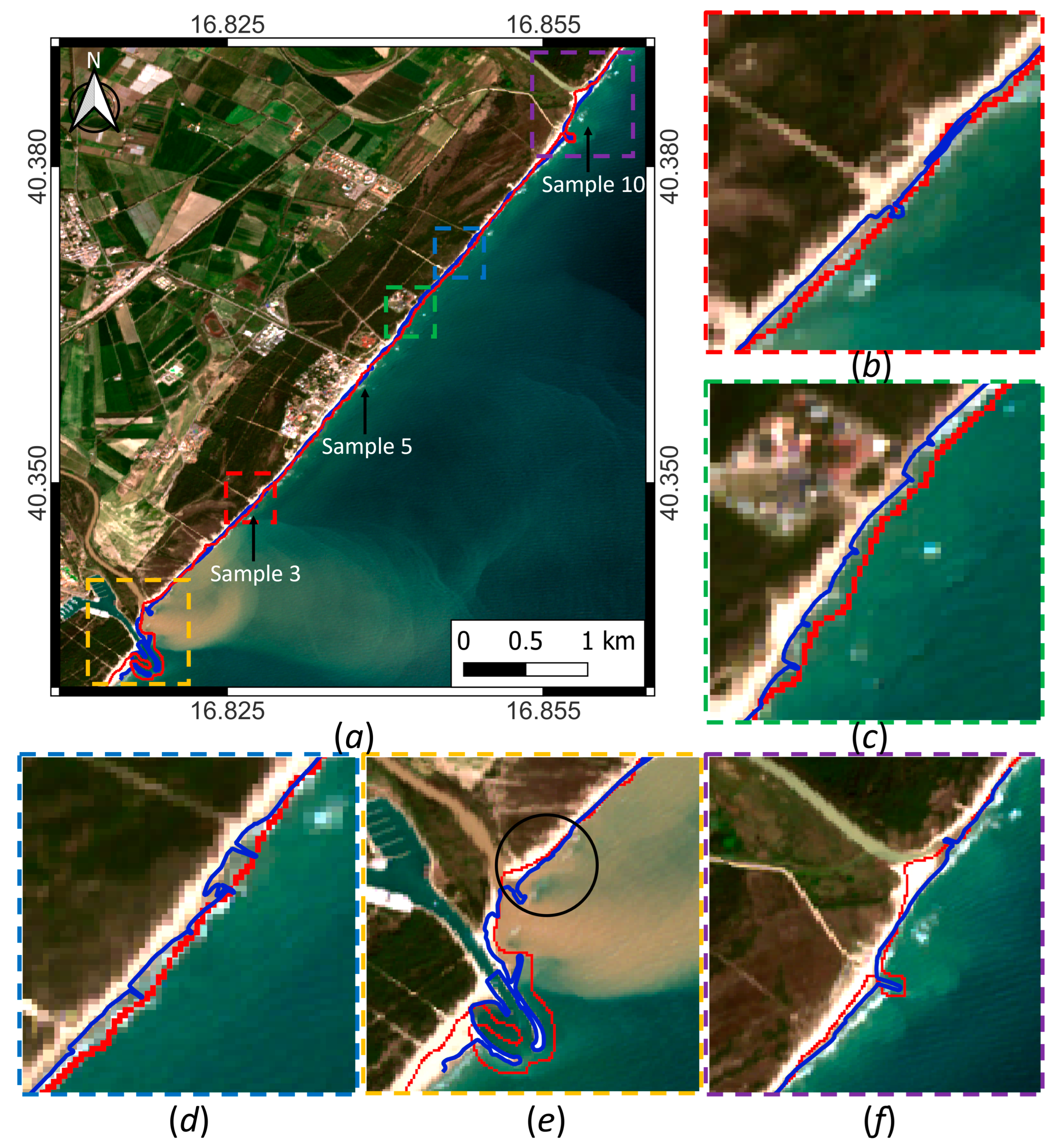
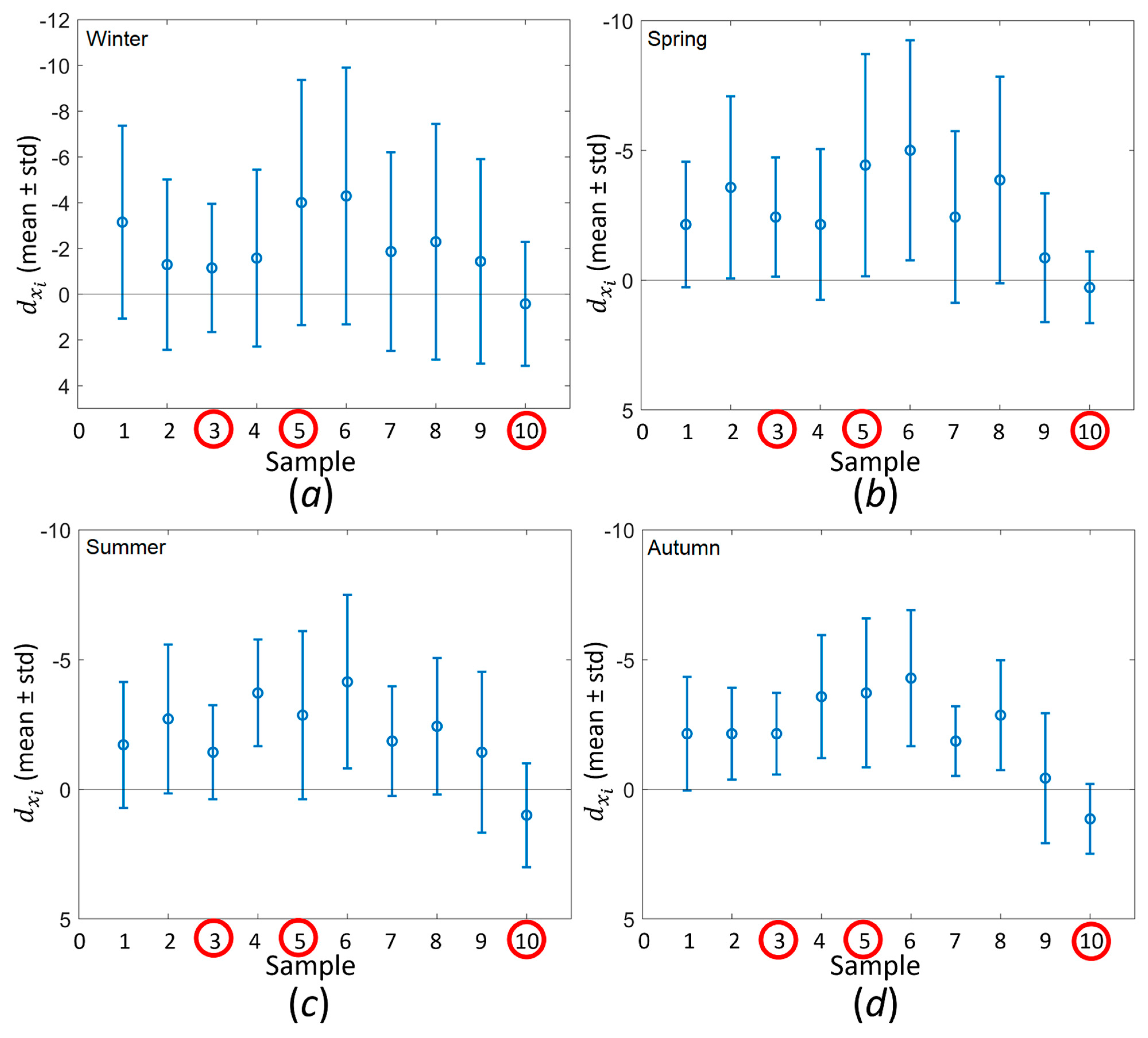
4.1. Accuracy Analysis

This subsection exists to discuss the accuracy of the coastline extracted by SAR using the coastline extracted from LIDAR measurements. When dealing with the SAR, the coastline is extracted over the area of interest using the SAR scene acquired on 12 April 2022 (see Table 1). The coastline is extracted using the processing chain described in the schematic of Figure 2. When dealing with the LIDAR, the coastline is extracted according to the procedure described in the Methodologies section.
The coastlines extracted using the SAR and LIDAR measurements are superimposed as red (SAR) and blue (LIDAR) lines onto the graytone intensity VV SAR image collected on 12 April 2022; see Figure 5. By visually inspecting the two lines, good agreement applies between the extracted coastlines. Note that, for visualization purposes, the SAR scene has been manually equalized to maximize the land/sea backscattering separation. The SAR and LIDAR coastlines are overlapping almost everywhere, with the exception of some areas where deviations are observed. To better analyze the coastlines, an excerpt of the true-color optical image collected using Sentinel-2 on 9 April 2022 that includes the area of interest is depicted in Figure 6a, where the SAR and LIDAR coastlines are coded using red and blue colors, respectively. The image confirms that the two coastlines overlap almost everywhere, with the exception of some areas where deviations occur.
To better discuss the behaviors of the two coastlines, five regions of interest (ROIs) are selected (see boxes in Figure 6a), where the two coastlines are superimposed onto the Sentinel-2 true-color MSI image for reference purposes. Enlarged versions of the boxes are displayed in Figure 6b–f. The zoomed-in versions of the ROIs show, in general, that the SAR-based coastline is more seaward than the LIDAR-extracted profile. This deviation is the largest in the ROI of Figure 6c,d. This is likely due to the saw tooth shape of the coastal area that can be observed by finer-spatial resolution LIDAR measurements, while its results are smoothed in the SAR imagery. A similar issue appears in Figure 6e, where the small-scale man-made infrastructures are well observed by the LIDAR coastline while they are detected as unique smoother structures at the SAR spatial resolution scale. It is also interesting to note that the sandy dune next to the river mouth (see Figure 6f) is not correctly identified by the SAR since it calls for a backscatter intensity that is almost indistinguishable from the sea. In fact, both the sandy dune and the sea surface call for Bragg or tilted-Bragg scattering.
This qualitative intercomparison between the SAR and LIDAR coastlines shows that non-cooperative satellite SAR acquisitions can be successfully used to extract the coastline with fairly good accuracy. The main deviation of the SAR coastline from the superimposed LIDAR measurements results from areas where the coast profile calls for a variability that cannot be observed at the SAR moderate spatial resolution. In addition, deviations may occur over areas where the land and sea are not sufficiently distinguished in terms of signal backscatter.
To provide a quantitative analysis of the SAR-based coastline with respect to the LI- DAR one, the distance between 250 peer points randomly selected onto the two coastlines is evaluated. The mean standard deviation distance (in meters) is equal to 14.16 ± 14 m. This score shows the remarkable accuracy of the SAR-based coastline extraction methodology, which, unlike the LIDAR one, relies on completely non-cooperative measurements and is partially unsupervised, i.e., just simple image processing refinements are needed to remove the false edges that may appear over both the land and sea.

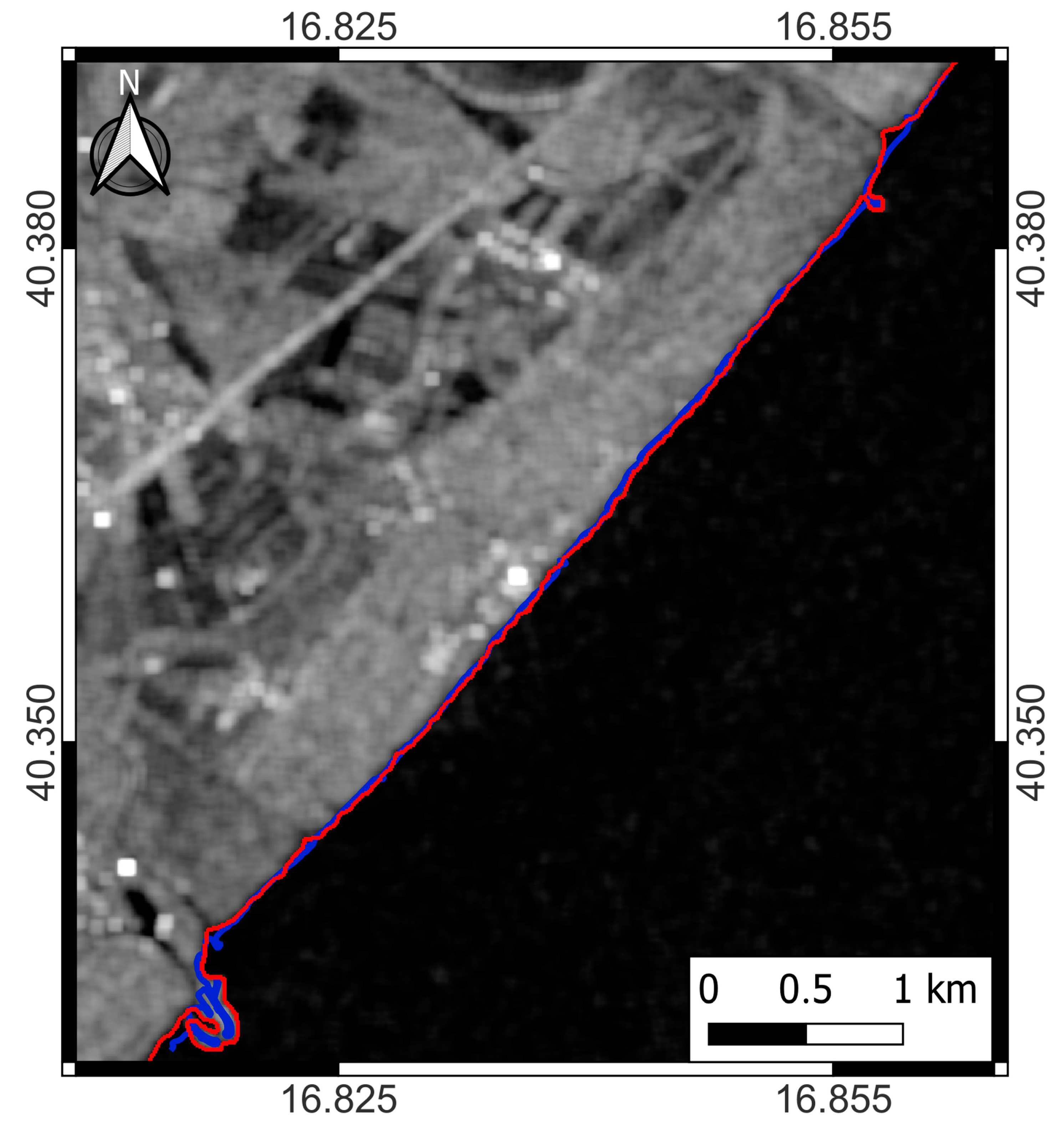
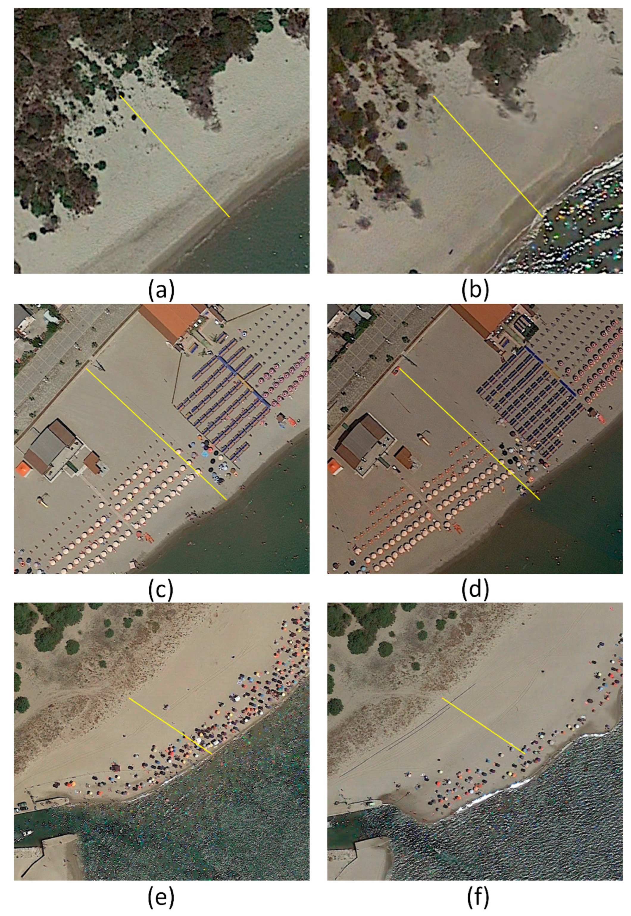
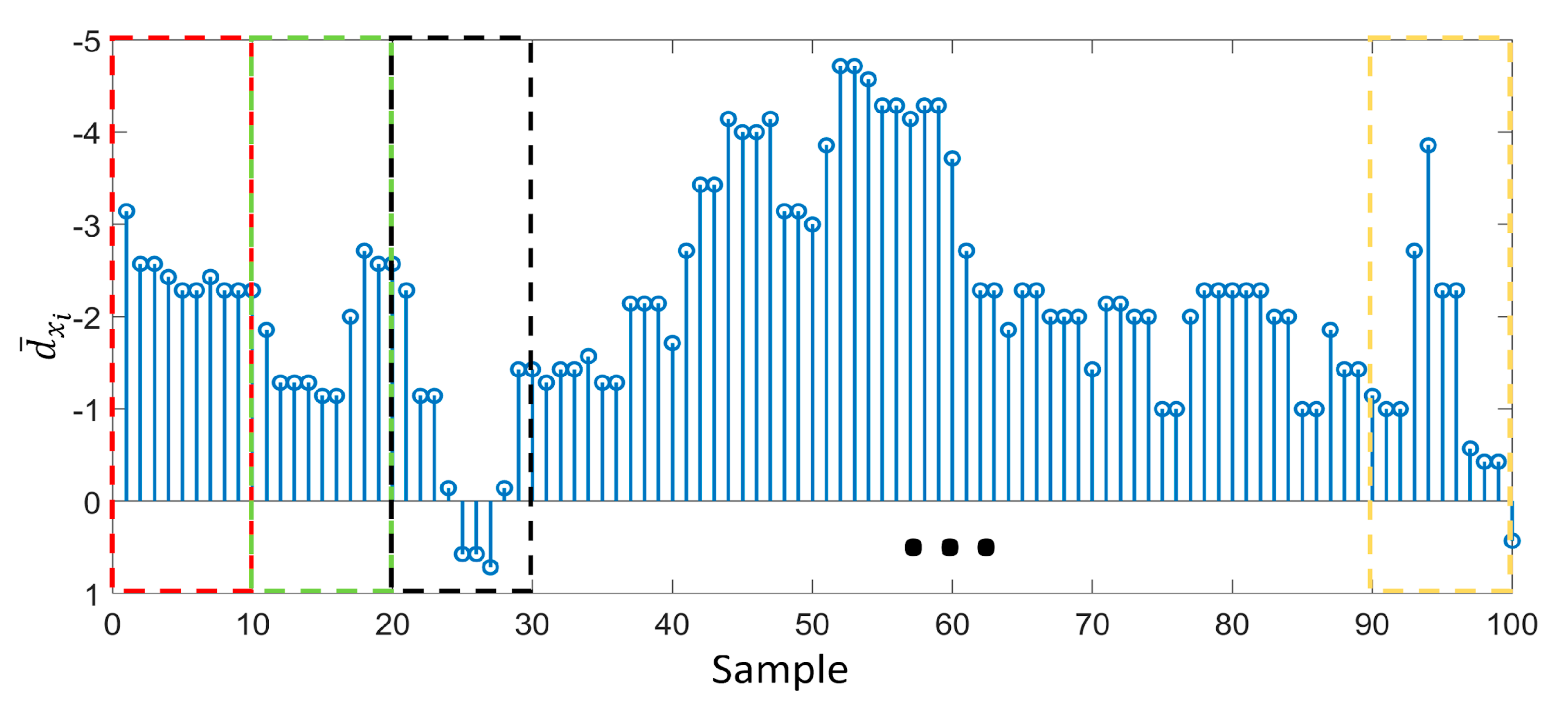
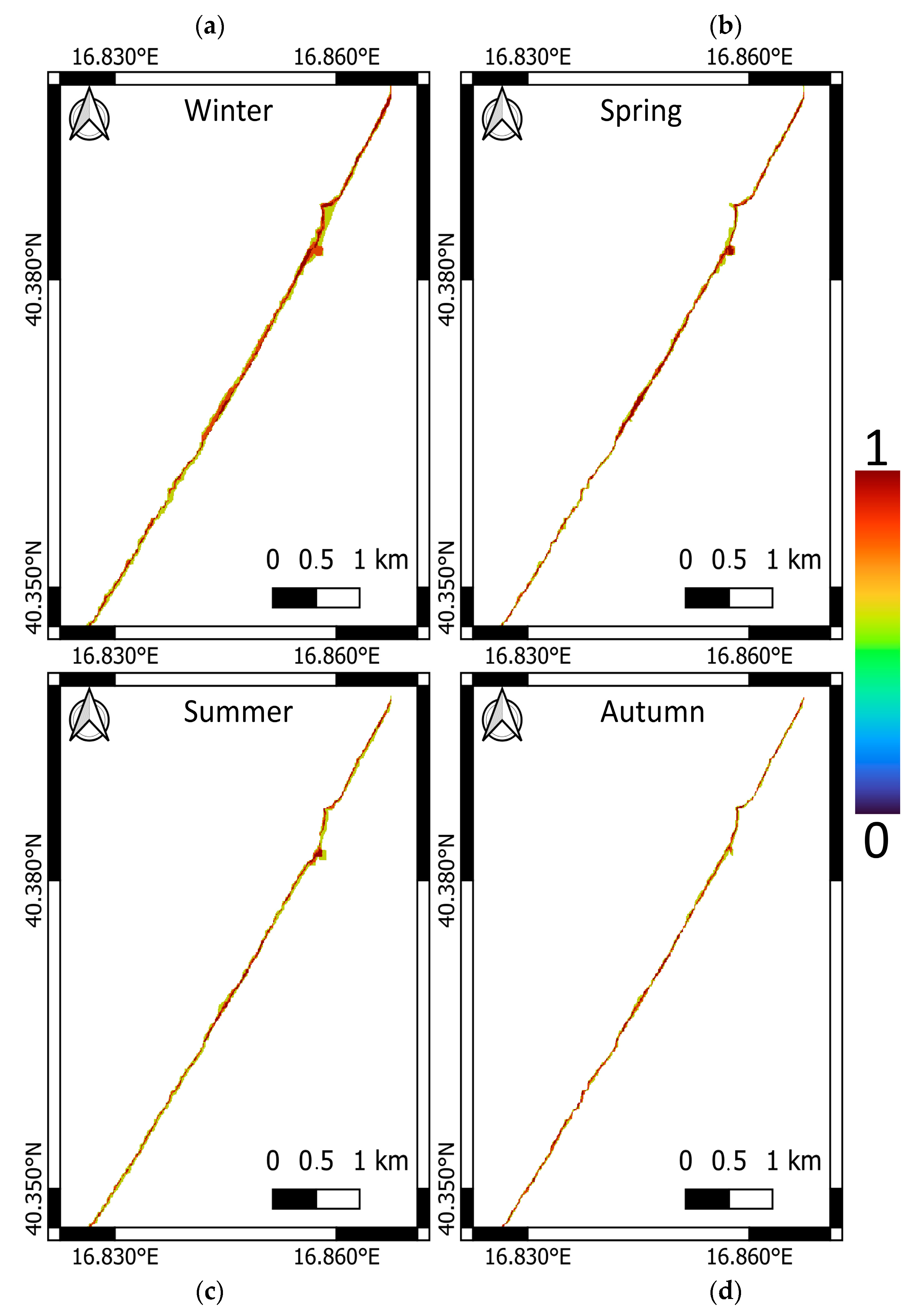
4.2. Time Variability of the Extracted Coastlines

This section describes the time-variability of the coastline related to the area of interest and extracted from the whole time series of the 28 Sentinel-1 SAR scenes.
The analysis is carried out by selecting 100 equally spaced samples from the coastlines extracted from each season (one per season). The samples are then averaged and decimated to obtain 10 equally spaced samples for each season. The time variability of the extracted coastlines is obtained by measuring the distance dxi of each sample from its peer, which is assumed to belong to the reference coastline, i.e., the coastlines extracted from the SAR scenes collected on 13 January 2015, 1 May 2015, 24 July 2015 and 28 October 2015 for winter, spring, summer and autumn, respectively. The dxi metric is displayed (in pixel) in Figure 7 as an error bar plot, where the circle and the bar stand for the mean value and standard deviation, respectively. The figure includes four panels ((a)–(d)) that are related to winter, spring, summer and autumn, respectively. Note that the negative and positive dxi values stand for erosion and accretion, respectively, and the y-axis is always oriented in such a way that the negative values (that stand for erosion) are displayed above zero. The results show that the dominant phenomenon is erosion. The mean values of the distances, for each season, show an oscillating trend and are always below 6 pixels. This behavior is very oscillating for all of the seasons, with the exception of autumn, which shows a piecewise-constant trend. It is also interesting to note that in all of the seasons (with the exception of winter), the last sample (i.e., the number 10) calls for accretion since it exhibits a positive distance. It is also worth noting that each sample calls for a large standard deviation. The latter is the largest in the winter and spring seasons, and this is likely due to the sea state conditions that may call for a larger number of high-sea-state events. The standard deviation decreases during the summer season, reaching the minimum during the autumn season. Note that the data set selected in this study calls for a low-to-moderate sea state condition, in accordance with the information provided by the corresponding Level 2 Sentinel-1 Ocean (OCN) data set. It is worth noting that sea state conditions can be also evaluated from SAR imagery [27,28].

5. Discussion

The experimental analysis demonstrates that the SAR-based coastline is reliable and accurate enough to observe the time variability of the coastline of the Ionian part of the Basilicata region. The time variability depicted in Figure 7 suggests a moderate cumulative erosion process that affects the area of interest in a non-uniform way with the area that corresponds to samples 5 to 7 suffering from the largest erosion and also exhibiting the largest variability, while the area that is less affected from erosion corresponds to sample 3. In addition, an accretion process can be appreciated by focusing on sample 10. Regarding verifying the time variability of the samples depicted in Figure 7, unfortunately, ground information is not available. Hence, a qualitative analysis is carried out that consists of using Google Earth imagery. The latter are acquired over the area of interest and are used to assist the physical interpretation of the time variability of the samples (sample 3, sample 5 and sample 10) enclosed in red circles in Figure 7. These samples are selected since they call for an erosion process characterized by the lowest (sample 3) and the largest (sample 5) time variability. Sample 10 calls for an accretion process. The location of the selected samples over the area of interest is annotated in Figure 6a. To better appreciate the type of scenario that the selected samples belong to and to discuss the dynamic of the coastline, Google Earth images acquired on two different dates are selected and depicted in Figure 8. The latter is organized in a matrix format where the columns stand for Google Earth optical images collected before and after the erosion or accretion phenomena, respectively. The rows stand for samples 3, 5 and 10, respectively. Note that, in Figure 8, for each row, an equal-length yellow line is annotated over the images to better appreciate the variability of the coastline. With respect to sample 3, the Google Earth optical images collected on 29 August 2015 and 8 July 2017 are shown in Figure 8a,b, respectively. The visual intercomparison suggests a very low variability of the coast (erosion of around 1 m) can be appreciated. With respect to sample 5, the Google Earth optical images collected on 8 July 2017 and 19 July 2018 are shown in Figure 8c,d, respectively. In this case, a higher erosion phenomenon can be observed (around 6 m). With respect to sample 10, the Google Earth optical images collected on 31 July 2016 and 8 July 2017 are shown in Figure 8e,f, respectively. The visual intercomparison suggests an accretion phenomenon of around 12 m. The qualitative analysis undertaken on samples 3, 5, and 10 confirms the time-variability analysis depicted in Figure 7.
The spatial distribution of the erosion process across the area of interest oscillates across the seasons. To discuss the spatial variability of the samples belonging to the extracted waterlines, 100 equally spaced samples are selected, as previously discussed. The mean value of the dxi metric is evaluated for each sample while considering, as a reference, the sample belonging to the coastline related to the SAR scene collected on 13 January 2015. The dxi values are then averaged to obtain the d _ x i metric, using 10 samples from non-overlapping windows (see Figure 9), where the d _ x i metric is illustrated with reference to the winter season. The mean and standard deviation of the 10 samples resulting from the averaging process are depicted in the error bar plots of Figure 10, where, again, panels (a–d) stand for winter, spring, summer and autumn, respectively. The plots of Figure 10 suggest the high spatial variability of the samples across the 10-sample window with the exception of a few samples. This variability is likely related to both the intrinsic error resulting from the SAR coastline extraction process and the inherent spatial variability of the coast profile that, as witnessed in Figure 6, exhibits very sharp changes that are not correctly identified at the Sentinel-1 SAR resolution scale.
To discuss the time variability of the whole coastline, a metric based on Shannon Entropy H is used. The metric is evaluated for each season using the whole time series. According to [29], H is defined as follows:
H ( x ) = k = 1 N p k x i l o g ( p k x i )
where
p k x i = P r o b ( x i = X )
is the probability that the pixel i of the k t h input image x is equal to X along the whole time series and N = 7 is the number of SAR scenes in the seasonal time series (one per year).
Hence, first, the whole time series of the extracted coastlines is grouped according to the seasons; then, for each season, an image is generated that consists of the superposition of all the extracted coastlines. For each image, the metric H is evaluated, and the output is depicted in Figure 11, where the four panels stand for (a) winter, (b) spring, (c) summer and (d) autumn. The color of the line at a given spatial position indicates the variability of that pixel along the time series. Dark blue means that, at that position, all of the extracted coastlines call for a logical true value, i.e., that pixel belongs to the coastline in all of the time series of SAR imagery. The departures for this condition are inherent to larger H values. The width of the line provides information about the extension (in pixels) of the erosion/accretion process.

6. Conclusions

The intention of this study was to discuss the ability of a non-cooperative satellite’s all-day imagery and almost-all-weather microwave SAR imagery to assist decision makers in promoting the effective and sustainable planning of complex coastal environments.
To reach this goal, a challenging environment was selected, belonging to the Ionian coast of the Basilicata region, Southern Italy. The area of interest is challenging for the unsupervised extraction of the coastline from remotely sensed imagery, which includes different kinds of beaches, river mouths and built-up areas.
First, we checked the accuracy of the coastline extracted from the SAR imagery by intercomparing the SAR-based coastline with a very accurate coastline extracted using drone-based LIDAR measurements, which were collected over the area of interest through a tailored field campaign. An accuracy finer than 15 m was obtained, which suggests that the satellite SAR measurements can be used to monitor the time variability of the coastline. Hence, we extracted the coastline using a time series of 28 SAR images acquired over the area of interest from 2015 to 2021 by the European Copernicus Sentinel-1 C-band SAR mission, and we discussed the time variability of the extracted coastline using tailored quantitative metrics. The experimental results show that, although the cumulative erosion process is within 6 pixels over the whole time period, significant deviations occur that are qualitatively verified against optical Google Earth imagery.
This underlines the efficacy of using satellite SAR imagery to support the monitoring and sustainable development of coastal environments. The results also suggest a joint use of long-range, i.e., satellite, and short-image, i.e., drone, surveys to map the coastline variability on both moderate- and fine-resolution spatial scales. The long-range observations could be used to point out anomalies that call for an in-depth analysis to be carried out using short-image surveys.

Author Contributions

Conceptualization, E.F., N.A.F. and F.N.; methodology, E.F., N.A.F. and F.N.; software, E.F., N.A.F. and F.N.; validation, all authors; formal analysis, all authors; investigation and data curation, all authors; writing—original draft preparation, all authors; writing—review and editing, all authors. All authors have read and agreed to the published version of the manuscript.

Funding

This research received no external funding.

Acknowledgments

This study was supported by the ESA-NRSCC cooperation project “Dragon 5”, with the project ID 57979—“Monitoring harsh coastal environments and ocean surveillance using radar remote sensing sensors” and the Regione Basilicata project “Aggiornamento Piano Regionale delle Coste”.

Conflicts of Interest

The authors declare no conflict of interest.

References

  1. Bird, E.C.F. Coastal Erosion and Rising Sea-Level. In Sea-Level Rise and Coastal Subsidence: Causes, Consequences, and Strategies; Milliman, J.D., Haq, B.U., Eds.; Coastal Systems and Continental Margins; Springer: Dordrecht, The Netherlands, 1996; pp. 87–103. ISBN 978-94-015-8719-8. [Google Scholar]
  2. Pellicani, R.; Argentiero, I.; Fidelibus, M.D.; Zanin, G.M.; Parisi, A.; Spilotro, G. Dynamics of the Basilicata Ionian Coast: Human and Natural Drivers. Rend. Fis. Acc. Lincei 2020, 31, 353–364. [Google Scholar] [CrossRef]
  3. Pardo-Pascual, J.E.; Almonacid-Caballer, J.; Ruiz, L.A.; Palomar-Vázquez, J. Automatic Extraction of Shorelines from Landsat TM and ETM+ Multi-Temporal Images with Subpixel Precision. Remote Sens. Environ. 2012, 123, 1–11. [Google Scholar] [CrossRef]
  4. Janušaitė, R.; Jukna, L.; Jarmalavičius, D.; Pupienis, D.; Žilinskas, G. A Novel GIS-Based Approach for Automated Detection of Nearshore Sandbar Morphological Characteristics in Optical Satellite Imagery. Remote Sens. 2021, 13, 2233. [Google Scholar] [CrossRef]
  5. Chi, S.; Zhang, C.; Zheng, J. Sandy Shoreline Recovery Ability after Breakwater Removal. Front. Mar. Sci. 2023, 10, 1191386. [Google Scholar] [CrossRef]
  6. Lee, J.; Jurkevich, I. Coastline Detection And Tracing In SAr Images. IEEE Trans. Geosci. Remote Sens. 1990, 28, 662–668. [Google Scholar] [CrossRef]
  7. Pelich, R.; Chini, M.; Hostache, R.; Matgen, P.; López-Martinez, C. Coastline Detection Based on Sentinel-1 Time Series for Ship- and Flood-Monitoring Applications. IEEE Geosci. Remote Sens. Lett. 2021, 18, 1771–1775. [Google Scholar] [CrossRef]
  8. Niedermeier, A.; Romaneessen, E.; Lehner, S. Detection of Coastlines in SAR Images Using Wavelet Methods. IEEE Trans. Geosci. Remote Sens. 2000, 38, 2270–2281. [Google Scholar] [CrossRef]
  9. Sheng, G.; Yang, W.; Deng, X.; He, C.; Cao, Y.; Sun, H. Coastline Detection in Synthetic Aperture Radar (SAR) Images by Integrating Watershed Transformation and Controllable Gradient Vector Flow (GVF) Snake Model. IEEE J. Ocean. Eng. 2012, 37, 375–383. [Google Scholar] [CrossRef]
  10. Baselice, F.; Ferraioli, G. Unsupervised Coastal Line Extraction From SAR Images. IEEE Geosci. Remote Sens. Lett. 2013, 10, 1350–1354. [Google Scholar] [CrossRef]
  11. Yu, Y.; Acton, S.T. Automated Delineation of Coastline from Polarimetric SAR Imagery. Int. J. Remote Sens. 2004, 25, 3423–3438. [Google Scholar] [CrossRef]
  12. Modava, M.; Akbarizadeh, G.; Soroosh, M. Integration of Spectral Histogram and Level Set for Coastline Detection in SAR Images. IEEE Trans. Aerosp. Electron. Syst. 2019, 55, 810–819. [Google Scholar] [CrossRef]
  13. Baghdadi, N.; Pedreros, R.; Lenotre, N.; Dewez, T.; Paganini, M. Impact of Polarization and Incidence of the ASAR Sensor on Coastline Mapping: Example of Gabon. Int. J. Remote Sens. 2007, 28, 3841–3849. [Google Scholar] [CrossRef]
  14. Moon, W.M.; Staples, G.; Kim, D.; Park, S.-E.; Park, K.-A. RADARSAT-2 and Coastal Applications: Surface Wind, Waterline, and Intertidal Flat Roughness. Proc. IEEE 2010, 98, 800–815. [Google Scholar] [CrossRef]
  15. Kim, D.; Moon, W.M.; Park, S.-E.; Kim, J.-E.; Lee, H.-S. Dependence of Waterline Mapping on Radar Frequency Used for SAR Images in Intertidal Areas. IEEE Geosci. Remote Sens. Lett. 2007, 4, 269–273. [Google Scholar] [CrossRef]
  16. Ding, X.; Nunziata, F.; Li, X.; Migliaccio, M. Performance Analysis and Validation of Waterline Extraction Approaches Using Single- and Dual-Polarimetric SAR Data. IEEE J. Sel. Top. Appl. Earth Obs. Remote Sens. 2015, 8, 1019–1027. [Google Scholar] [CrossRef]
  17. Nunziata, F.; Buono, A.; Migliaccio, M.; Benassai, G. Dual-Polarimetric C- and X-Band SAR Data for Coastline Extraction. IEEE J. Sel. Top. Appl. Earth Obs. Remote Sens. 2016, 9, 4921–4928. [Google Scholar] [CrossRef]
  18. Ferrentino, E.; Nunziata, F.; Migliaccio, M. Full-Polarimetric SAR Measurements for Coastline Extraction and Coastal Area Classification. Int. J. Remote Sens. 2017, 38, 7405–7421. [Google Scholar] [CrossRef]
  19. Schmitt, M.; Baier, G.; Zhu, X.X. Potential of Nonlocally Filtered Pursuit Monostatic TanDEM-X Data for Coastline Detection. ISPRS J. Photogramm. Remote Sens. 2019, 148, 130–141. [Google Scholar] [CrossRef]
  20. Xue, W.; Yang, H.; Wu, Y.; Kong, P.; Xu, H.; Wu, P.; Ma, X. Water Body Automated Extraction in Polarization SAR Images With Dense-Coordinate-Feature-Concatenate Network. IEEE J. Sel. Top. Appl. Earth Obs. Remote Sens. 2021, 14, 12073–12087. [Google Scholar] [CrossRef]
  21. Scharf, L.L.; Demeure, C. Statistical Signal Processing: Detection, Estimation, and Time Series Analysis; Addison-Wesley Publishing Company: Boston, MA, USA, 1991; ISBN 978-0-201-19038-0. [Google Scholar]
  22. Bandini, F.; Sunding, T.P.; Linde, J.; Smith, O.; Jensen, I.K.; Köppl, C.J.; Butts, M.; Bauer-Gottwein, P. Unmanned Aerial System (UAS) Observations of Water Surface Elevation in a Small Stream: Comparison of Radar Altimetry, LIDAR and Photogrammetry Techniques. Remote Sens. Environ. 2020, 237, 111487. [Google Scholar] [CrossRef]
  23. Thayer, J.; Sacca, K.; Thompson, G.; Bukowski, S.; Garby, B. Novel UAS-Based LiDAR for Shallow-Water Bathymetry. In Proceedings of the AGU Fall Meeting 2021, New Orleans, LA, USA, 13–17 December 2021; Volume 2021, p. G55D-0277. [Google Scholar]
  24. Gisler, A.; Thayer, J.P.; Nderson, C.; Crowley, G. The First UAV-Borne Scanning Topographic and Bathymetric Lidar System for Mapping Coastal Regions. In Proceedings of the American Geophysical Union, Fall Meeting 2018, Washington, DC, USA, 10–14 December 2018; Volume 2018, p. EP52D-33. [Google Scholar]
  25. Szafarczyk, A.; Toś, C. The Use of Green Laser in LiDAR Bathymetry: State of the Art and Recent Advancements. Sensors 2023, 23, 292. [Google Scholar] [CrossRef] [PubMed]
  26. Famiglietti, N.A.; Cecere, G.; Grasso, C.; Memmolo, A.; Vicari, A. A Test on the Potential of a Low Cost Unmanned Aerial Vehicle RTK/PPK Solution for Precision Positioning. Sensors 2021, 21, 3882. [Google Scholar] [CrossRef] [PubMed]
  27. Zhang, B.; Perrie, W. Cross-Polarized Synthetic Aperture Radar: A New Potential Measurement Technique for Hurricanes. Bull. Am. Meteorol. Soc. 2012, 93, 531–541. [Google Scholar] [CrossRef]
  28. Benassai, G.; Migliaccio, M.; Montuori, A.; Ricchi, A. Wave Simulations Through Sar Cosmo-Skymed Wind Retrieval and Verification with Buoy Data. In Proceedings of the The Twenty-second International Offshore and Polar Engineering Conference, Rhodes, Greece, 17–22 June 2012. [Google Scholar]
  29. Shannon, C.E. A Mathematical Theory of Communication. Bell Syst. Tech. J. 1948, 27, 623–656. [Google Scholar] [CrossRef]
Figure 1. Pictorial view of the area that hosts the Ionian coast of the Basilicata region, Italy. The red rectangle shows the selected region of interest adopted in this study.
Environments 10 00212 g001
Figure 2. Flowchart showing the coastline extraction methodology starting from a dual-pol VV + VH Sentinel-1 acquisition.
Environments 10 00212 g002
Figure 3. The area of interest on Basilicata’s Ionian coast, Southern Italy.
Environments 10 00212 g003
Figure 4. Pictorial view of the 7 flight paths performed on 12 April 2022. The paths are annotated over the Google Earth image of the area of interest. The take-off/landing locations are marked as red/green arrows, while the air/ground flight paths are marked using green and yellow horizontal lines. The yellow vertical lines stand for the intermediate waypoints. The enlarged versions of the 7 paths are depicted in the 7 boxes.
Environments 10 00212 g004
Figure 5. Excerpt of the VV-polarized SAR scene acquired on 12 April 2022, where the SAR- (red) and LIDAR-extracted (blue) coastlines are annotated.
Environments 10 00212 g005
Figure 6. Sentinel-2 MSI true-color image collected over the area of interest on 9 April 2022. (a) The SAR and LIDAR coastlines are superimposed on the optical image; see red and blue lines, respectively. Enlarged versions of the ROIs depicted in panel (a) are displayed in panels (b)–(d).
Environments 10 00212 g006
Figure 7. dxi metric (in pixel) shown as mean (circle) and standard deviation (bars) values related to winter (a), spring (b), summer (c) and autumn (d). Note that the samples selected for the visual interpretation discussed in Figure 8 are enclosed in red circles.
Environments 10 00212 g007
Figure 8. Google Earth images of the area that includes samples annotated in Figure 6a. The figure is organized in a matrix format where columns stand for Google Earth optical images collected before (a,c,e) and after (b,d,f) the erosion or accretion phenomena, respectively, while rows stand for samples 3 (a,b), 5 (c,d), and 10 (e,f), respectively. Panels (a), (b)–(c)–(f), (d) and (e) refer to images collected on 29 August 2015, 8 July 2017, 19 July 2018 and 31 July 2016, respectively.
Environments 10 00212 g008
Figure 9. Sketch of the methodology applied to discuss the spatial variability of the 10 samples. The boxes depicted using dashed lines represent the averaging process.
Environments 10 00212 g009
Figure 10. d _ x i metric (in pixel) shown as mean (circle) and standard deviation (bars) values related to winter (a), spring (b), summer (c) and autumn (d) and evaluated according to the procedure sketched in Figure 9.
Environments 10 00212 g010
Figure 11. H metric evaluated over the whole time series of extracted coastlines and arranged according to the seasons: winter (a), spring (b), summer (c) and autumn (d).
Environments 10 00212 g011
Table 1. SAR, drone and ancillary data sets.
SensorAcquisition Date
(dd/mm/yyyy)
Resolution (m)SeasonLIDAR Measurement
Sentinel-128/10/201510AutumnNo
Sentinel-113/01/201510WinterNo
Sentinel-101/05/201510SpringNo
Sentinel-124/07/201510SummerNo
Sentinel-120/01/201610WinterNo
Sentinel-119/05/201610SpringNo
Sentinel-111/08/201610SummerNo
Sentinel-109/11/201610AutumnNo
Sentinel-108/01/201710WinterNo
Sentinel-102/04/201710SpringNo
Sentinel-106/08/201710SummerNo
Sentinel-117/10/201710AutumnNo
Sentinel-115/01/201810WinterNo
Sentinel-121/04/201810SpringNo
Sentinel-101/08/201810SummerNo
Sentinel-124/10/201810AutumnNo
Sentinel-104/01/201910WinterNo
Sentinel-122/04/201910SpringNo
Sentinel-102/08/201910SummerNo
Sentinel-119/10/201910AutumnNo
Sentinel-111/01/202010WinterNo
Sentinel-128/04/202010SpringNo
Sentinel-102/08/202010SummerNo
Sentinel-125/10/202010AutumnNo
Sentinel-105/01/202110WinterNo
Sentinel-111/04/202110SpringNo
Sentinel-110/07/202110SummerNo
Sentinel-120/10/202110AutumnNo
Sentinel-112/04/202210SpringYes
Sentinel-209/04/202220SpringNo
Google Earth29/08/2015N/ASummerNo
Google Earth31/07/2016N/ASummerNo
Google Earth08/072017N/ASummerNo
Google Earth19/07/2018N/ASummerNo
Disclaimer/Publisher’s Note: The statements, opinions and data contained in all publications are solely those of the individual author(s) and contributor(s) and not of MDPI and/or the editor(s). MDPI and/or the editor(s) disclaim responsibility for any injury to people or property resulting from any ideas, methods, instructions or products referred to in the content.

