Article

Soil Organic Carbon Estimation in Ferrara (Northern Italy) Combining In Situ Geochemical Analyses and Hyperspectral Remote Sensing

1
Department of Chemical, Pharmaceutical and Agricultural Sciences, University of Ferrara, 44121 Ferrara, Italy
2
Department of Physics and Earth Sciences, University of Ferrara, 44122 Ferrara, Italy
3
MEEO Srl, 44121 Ferrara, Italy
4
Department of Geography, University of Colorado Boulder, Boulder, CO 80309, USA
5
SISTEMA GmbH, 1010 Vienna, Austria
6
Department of Earth Sciences, University of Florence, 50121 Florence, Italy
*
Author to whom correspondence should be addressed.
Environments 2023, 10(10), 173; https://doi.org/10.3390/environments10100173
Submission received: 3 September 2023 / Revised: 28 September 2023 / Accepted: 2 October 2023 / Published: 4 October 2023

Abstract

:
This study investigated whether surface soil organic carbon (SOC) content could be estimated using hyperspectral data provided by the Italian Space Agency PRISMA satellite. We collected 100 representative topsoil samples in an area of 30 × 30 Km2 in the province of Ferrara (Northern Italy), estimated their SOC content and other soil properties through thermo-gravimetric analysis, and matched these to the spectra of the sampled areas that were measured by PRISMA on 7 April 2020. A tentative model was created for SOC estimation using ordinary least-squares (OLS) regression and an artificial neural network (ANN). Repeated k-fold cross-validation of the OLS and ANN models yielded R2 values of 0.64 and 0.49, respectively. The performance of the models was inferior to that obtained from the literature using similar modeling techniques in relatively small areas (up to 3 × 3 Km2) and characterized by restricted SOC variability (0.2–2.1 wt%). However, our data were collected over a wider area with high SOC content variability (0.7–9.3 wt%); consequently, significant variations were observed over a spatial scale of just a few meters. Therefore, this work shows the importance of testing remote sensing techniques for SOC measurements in more complex areas than those reported in the existing literature. Furthermore, our study sheds light on the geolocation errors and missing data of PRISMA.

1. Introduction

The earth critical zone (CZ) is a variable thickness layer composed of soil, rocks, air, and biota, which is constrained between the treetops and the groundwater bottom [1,2]. It has an evolving nature that is constantly modified by the interaction of environmental matrices and related biogeochemical processes [3]. Only the shallowest portion of the CZ can be directly modified by human activities, in particular by intensive agricultural practices, which interfere with natural CZ transformations, causing soil and plant degradation. In this context, monitoring the complexity of CZ processes and the impact of human activities is fundamental. In particular, geochemistry can offer a picture of the environmental conditions of the CZ, providing the elemental concentrations for all the involved matrices (water, soil, and air) and also ensuring replicable methods to monitor changes. Focusing on soil properties, soil organic carbon (SOC), which represents ~50% of soil organic matter (SOM), is considered a proxy of soil quality and fertility [4]. The organic carbon pool is composed of living and dead organic materials, and its presence in soil facilitates soil aggregation, consequently affecting soil erosion, aeration, water balance, temperature, root growth, and biota activities, and also promotes crop productivity [5]. In addition, SOM represents an important carbon stock, whose preservation is essential to reduce greenhouse gas emissions, which increase global warming [6]. In this framework, the control of SOM conditions, especially in agriculture areas, has become a priority, to ensure the fertility of soils and for climate change mitigation. For this reason, innovative and fast approaches are urgently needed to monitor and map the SOC content of agricultural soils in wide areas.
Over the last decade, several authors [7,8,9,10,11] have described the rising interest in digital maps of SOC spatial distribution, which are useful in (i) defining a baseline of carbon level, (ii) providing soil information to farmers and policymakers, (iii) identifing areas with gain and loss of C; and (iv) feeding models with new data. Methods that have been used to estimate the spatial distribution of SOC include in situ measurements such as electrical conductivity and the spectroscopy of the soil at visible near infrared (VNIR) and short-wave infrared (SWIR) wavelengths [12]. Spectroscopic analysis carried out in laboratories has made it possible to construct soil spectral libraries (e.g., ISRIC World Soil Reference Collection [13]; LUCAS [14]; USDA Rapid Carbon Assessment [15,16]), which have been used to predict SOC distribution at large scales. However, libraries have to be constantly improved to take into account local factors that are bypassed and not considered in earlier versions. Since detailed spectral libraries often originate from local studies built independently using different protocols for soil and spectral analyses, SOC predictions for bigger areas using these libraries are often inaccurate [17]. Spectroscopy can alternatively be carried out using remote spaceborne sensors (e.g., [18,19]). Remote satellite spectroscopy can be an inexpensive way to quantify SOC concentration quickly. These methods still require complex statistical processing and modeling [20] and, in spite of continuous improvements in sensor technology, they remain constrained by sources of noise such as soil roughness, soil moisture, and vegetation cover [12]. Nevertheless, the accuracy of SOC estimation methods that rely on remotely sensed soil spectra is currently increasing [12,21,22,23,24].
In our study, we explored the potential of hyperspectral spaceborne sensors for predicting SOC. These sensors are characterized by 200+ bands and can thus sample spectra with a very fine spectral resolution. In particular, we have largely reprised the processing and modeling methods used by Meng et al. [24], applying them to 100 topsoil samples (0–15 cm in depth), which we gathered in the province of Ferrara, and to the soil spectra detected in the sampling locations by the Italian Space Agency hyperspectral satellite PRISMA [25]. Ferrara province is characterized by wide SOC variability, as it hosts different environments from medium-textured soils with low SOM contents to peat soil with high SOM contents, resulting from the drainage of the province in the XX century [26]. In addition, this area, like the rest of the territories of the Padanian Plain, is intensively used for agriculture; therefore, a digital map of SOC is in the interest of local farmers, as well as for policymakers to plan future land use.

2. Materials and Methods
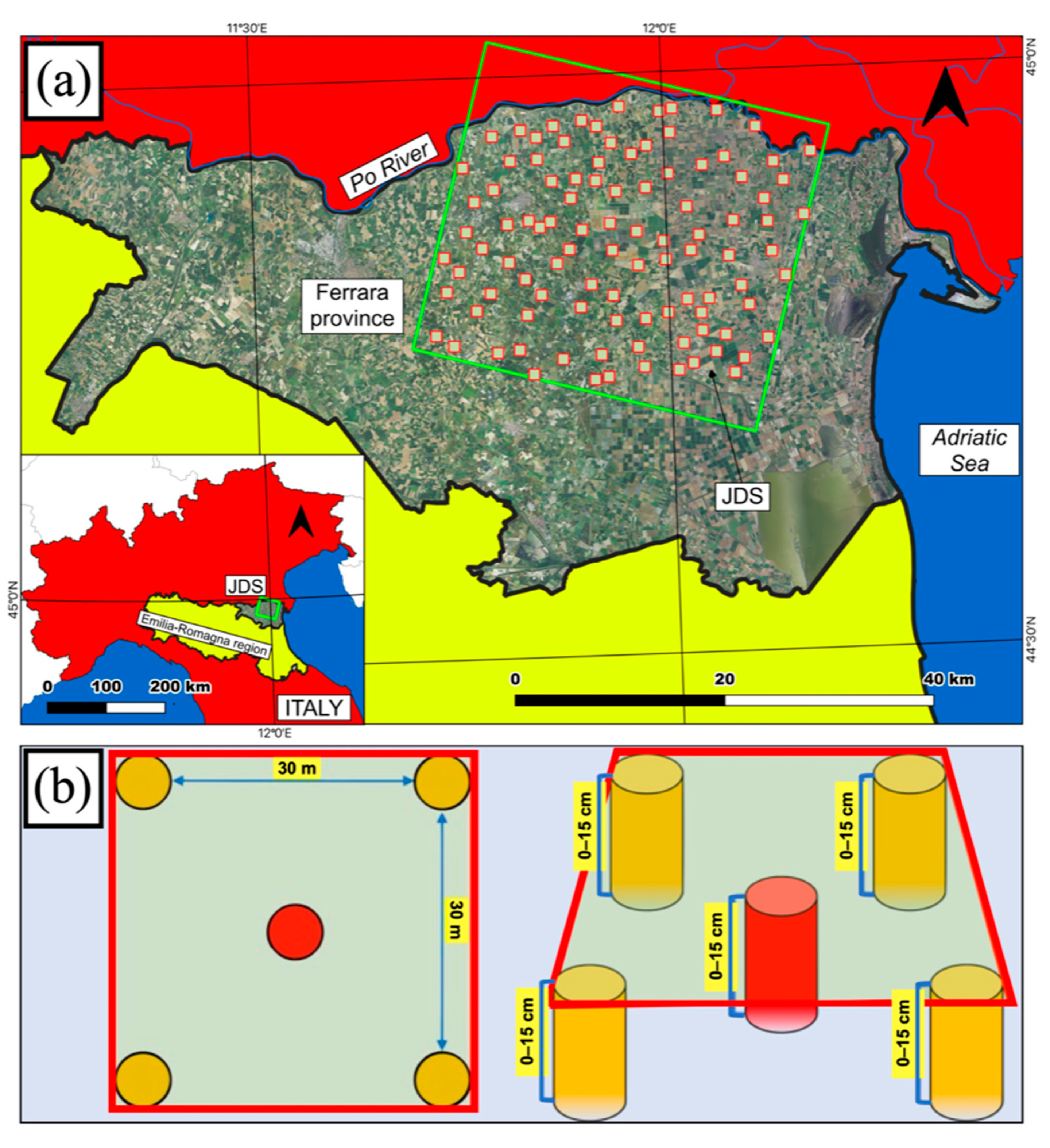
2.1. Study Area

This study was carried out in the area surrounding the municipality of Jolanda di Savoia (JDS) in Ferrara province in Northern Italy (Emilia-Romagna region; Figure 1a). Overall, Ferrara province has a surface of ~2636 km2 and is located south of the Po River and in the easternmost part of the Padanian plain (Figure 1a). The territory is occupied by alluvial, deltaic, and coastal plains [27] formed during the Holocene (<10,000 years) by the Po and Apennine Rivers (i.e., the Reno River and its tributaries), which contributed to the infilling of the Padanian plain, and by coastal remodeling in the east [28]. Complex and various geomorphologies such as paleo-channels, crevasses splay, and marsh lagoon environments are therefore widespread [26,29,30], and this is reflected in the textural composition of the main soil types, which vary as follows: medium-fine-textured soils (68% of the territory), medium-fine sands (9% of the territory), and peaty soils (23% of the territory) [26,28,29,31]. The current physiographic framework is the result of several drainage activities of the palustrine environment that were carried out up to the XX century [32,33].
As described by Colombani et al. [26], the prevalent land use in Ferrara province is agriculture, with ~50% of crops represented by winter cereals (~32%) and maize (~22%) and the remaining represented by rice paddy (especially in the reclaimed area of JDS), soybean, and horticulture.
Ferrara province has a sub-coastal temperate climate, mainly due to the proximity of the Adriatic Sea (Figure 1a). It is therefore characterized by cold winters and warm summers, elevated humidity, moderate precipitation, low wind speed, and moderate daily and seasonal temperature excursions [29].

2.2. PRISMA

PRISMA (PRecursore IperSpettrale della Missione Applicativa) is a pre-operational hyperspectral satellite mission of the Italian Space Agency (ASI). The satellite’s payload comprises a medium-resolution panchromatic camera and an imaging spectrometer. The former acquires panchromatic images in the 400–700 nm spectral range with a 5 m ground sampling distance (GSD), whereas the latter is designed to take images with a 30 m GSD in 66 bands in the VNIR spectral range (400–1010 nm) and 173 bands in the SWIR range (920–2500 nm), for a total of 239 bands [34]. The images acquired by PRISMA in each band are composed of 1000 × 1000 30 m pixels and hence cover an area of about 30 × 30 km2. The corresponding panchromatic image is, obviously, composed of 6000 × 6000 5 m pixels.
PRISMA data products available to the public include a level 1 (L1) product containing top-of-atmosphere (TOA) radiance data, which also includes a cloud cover mask, and three level 2 (L2) products containing bottom-of-atmosphere data obtained from the L1 products by applying an atmospheric correction algorithm. Specifically, the L2 products include at-surface radiance (L2B) and reflectance (L2C) data and a geocoded reflectance data product (L2D) where corrections have been implemented to account for collection geometry distortions and the terrain topography. We chose to work with surface reflectance data and, specifically, L2C images, avoiding L2D products because the geocoding process reprojects the data onto a new grid, whereas we wanted to preserve the original data collection geometry.

2.3. Available PRISMA Images and Soil Sampling

The JDS area was, as of March 2022, covered by 17 PRISMA images, 13 of which had cloud cover of < 10%. The reason for this abundance of acquisitions in the JDS municipality is the presence of a wide farmland area often used as a study area for remote sensing studies, particularly in the field of agriculture (e.g., [35]). We selected the PRISMA images that we would use in our analysis on the basis of its low cloud cover and of the abundance of bare soil pixels, with no vegetation cover. We made the assumption that the soil properties, and specifically the SOC content, would not have significantly changed since the image acquisition date.
To check the presence of a vegetation cover, we used Copernicus Sentinel-2 (European Space Agency) normalized difference vegetation index (NDVI) data. Sentinel-2 supplies global multispectral data with a spatial resolution of 10 m and a revisit time of 5 days. Sentinel-2 NDVI is computed as follows:
NDVI Sentinel-2 = (B08 − B04)/(B08 + B04)
where B04 and B08 are the red and near infrared Sentinel-2 bands, respectively.
We used a reserved API key on the ADAM Platform (https://adamplatform.eu; accessed on 6 December 2021) managed by MEEO Srl to download the Sentinel-2 NDVI time series for our study area in the period December 2016–December 2021.
We then focused specifically on the NDVI values observed on the dates closest to the acquisition dates of the PRISMA images. We set the NDVI upper limit for bare soil to 0.3 and classified the PRISMA images based on the fraction of bare soil within their extent at the time of their capture.
We thus concluded that the most suitable PRISMA image would be the one collected on 7 April 2020. On this image, we selected 100 bare soil 30 m pixels distributed across its extent and chose these as our soil sampling sites. Since the geolocation error for these pixels could sometimes exceed 30 m, we had to visually examine each pixel both in the 30 m hyperspectral and 5 m panchromatic images to identify features that would allow us to ascertain its actual location on the ground. The position of our 100 sampling sites is shown in Figure 1a. Table 1 shows how many of our sampling sites would have been free of vegetation cover had we used a different image or a different NDVI threshold.
Soil sampling was carried out in October 2021, under the assumption that the SOC content would not have changed significantly since April 2020. Since the SOC content could vary over a scale of just a few meters, and thus be lower than the 30 m PRISMA hyperspectral resolution, we collected 5 aliquots of topsoil (0–15 cm in depth) in each sampling location over the square parcel of 30 × 30 m2 which corresponded to the site’s PRISMA hyperspectral pixel (Figure 1b). The 5 aliquots were then mixed to create a composite sample. Sampling was carried out using a gouge auger (Eijkelkamp®, Zevenaar, The Netherlands).

2.4. Analyses of Soil Samples

2.4.1. Thermo-Gravimetric Analyses

At the Department of Physics and Earth Sciences of the University of Ferrara, soil samples were air-dried, sieved at <2 mm, and powdered using an agate mortar. Sequential loss on ignition (LOI) was performed by heating the soil samples in a muffle furnace at different temperatures [36]. The gypsum and hygroscopic water content (LOI 105 °C) was estimated after heating the soil samples at 105 °C for 12 h and calculated as follows:
LOI 105 °C (wt%) = (WS − DW105)/WS × 100
where WS is the air-dried weight and DW105 is the dry weight after heating at 105 °C.
After the evaluation of LOI 105 °C, the same soil samples were heated at 550 °C to determine the content of soil organic matter (LOI 550 °C) as follows:
LOI 550 °C (wt%) = (DW105 − DW550)/DW105 × 100
where DW105 is the dry weight after the heating at 105 °C and DW550 is the weight of the exsolved SOM.
Finally, the same soil samples were heated at 1000 °C to calculate the soil inorganic fraction (LOI 1000 °C) as follows:
LOI 1000 °C (wt%) = (DW550 − DW1000)/DW550 × 100
where DW550 is the dry weight after heating at 550 °C and DW1000 is the weight of the destabilized part of the inorganic fraction (carbonates and clay minerals).

2.4.2. Elemental Speciation of Carbon

The C fraction contents were measured on the powdered soil samples using an elemental analyzer Soli TOC Cube (Elementar®, Langenselbold, Germany) at CREA (Council for Agricultural Research and Economics, Gorizia, Italy). The analysis was carried out with a “smart combustion” method which allows the determination of total (TC), organic (SOC), and inorganic (SIC) carbon contents (wt%) [37]. As required by this method, the samples were heated to 600 °C under oxygen-rich conditions for the measure of the SOC contents, after which further heating was caried out under anoxic conditions until 900 °C for the measure of SIC contents. A standard of calcium carbonate (CaCO3, Calciumcarbonat, Elementar) and a soil standard (Bodenstandard, Elementar) were analyzed prior to, between, and after each run. The analytical precision and accuracy of the instrument were better than 5% of the absolute measured value [38].

2.5. Modeling

We used an artificial neural network (ANN) and ordinary least-squares (OLS) regression to model the relationship between the PRISMA spectra and the soil properties. We mainly used SOC as the output variable, but we also tested the other soil variables (which are not independent). The input variables were obtained from the soil spectra. We compared the performance of the ANN and OLS models using the R2 coefficient of determination obtained through repeated k-fold cross-validation.

2.5.1. Pre-Processing

We carried out a series of pre-processing steps to select the input variables for our model. In this, we imitated the procedure used by Meng et al. [24] in their work on SOC and Gaofen-5 hyperspectral data. The steps were as follows:
  • Valid bands: We removed from the PRISMA spectra the bands that were affected by missing data or that were outside atmospheric windows (Table 2).
  • First derivative: We computed the first derivative curve of each reflectance spectrum to remove noise and emphasize some spectral features that might have been concealed in the original curves. We carried out the subsequent preprocessing steps and the modeling operations using both the original spectra and the first derivative (FDR) spectra to check which ones would perform best.
  • Wavelet transform: We applied a discrete wavelet transform (DWT) to smooth the spectral curves. A DWT utilizes coupled high-pass and low-pass filters, which are applied to a curve yield a set of detail and approximation coefficients. The filters are then applied iteratively to the approximation coefficients l times, where l is the level of the DWT, ultimately yielding one set of approximation coefficients and l sets of detail coefficients. By then applying the inverted filters only to the approximation coefficients, a smoothed curve can be obtained. We applied a 3-level DWT using a Daubechies 4 wavelet.
  • PCA: We carried out a principal component analysis (PCA), using the smoothed curves. The components found by a PCA are the eigenvectors of the covariance matrix computed for all the bands under consideration, while their corresponding eigenvalues are their explained variances. We searched for a number of components whose total explained variance would be at least 0.85. We then used the eigenvector entries for each band to assign a weight to each band.
  • Spectral indices: For any two bands, we computed three spectral indices.
    NDI = (Ri − Rj)/(Ri + Rj)
    RI = Ri/Rj
    DI = Ri − Rj
    where: R is the spectral data and i ≠ j
  • Inputs: We used as “optimal” input variables the NDI, RI, and DI whose coefficients of correlation with the output variable were highest. To these, we added the three bands whose weights, computed in Step 4, were the highest. These were the 1595.9796 nm, 1575.3931 nm, and 1585.6315 nm bands for the original spectra and the 2462.813 nm, 2469.4155 nm, and 2476.7913 nm bands for the FDR spectra.

2.5.2. Neural Network

Artificial neural networks are a powerful and versatile machine learning system that can be configured to tackle a wide variety of tasks. The base unit of a neural network is an artificial neuron, a function that receives a series of numerical inputs, computes their weighted sum, adds an offset term, and then runs the result through a non-linear activation function. The most common neural network architecture, the multi-layer perceptron (MLP) is composed of artificial neurons arranged into multiple layers. The neurons of the first layer receive all the model’s input variables, while the neurons of the following layers, known as hidden layers, receive all the outputs of the previous layer. In a regression MLP, used to estimate a continuous variable like SOC content, the last layer is composed of a single neuron which takes the outputs of the previous layers and yields the estimated value of the output variable.
A neural network is trained by supplying it with a dataset of associated input and output variable values. In the course of the training process, the weights used by each neuron are adjusted until the model converges to a plateau level of accuracy.
We used an MLP configuration composed of 1 hidden layer of 12 neurons, like the one used by Meng et al. (2020) [24]. The other parameters of the configuration are displayed in Supplementary Table S1. The inputs were the six “optimal” variables defined in Section 2.5.1 and the output variables were the SOC value.

2.5.3. Ordinary Least-Squares Regression

In addition to the ANN, we also used a more conventional multivariate ordinary least-squares (OLS) regression. As inputs for the OLS model, we first used all the PRISMA bands, minus the ones indicated in Table 2. We then used the six “optimal” input variables.
In both cases, after fitting the full model, we used a stepwise algorithm to drop non-significant variables based on the Akaike information criterion (AIC). We then used a second stepwise algorithm to remove collinear variables whose variance inflation factor (VIF) exceeded 5. We then applied the AIC stepwise algorithm a second time to remove any remaining non-significant variables. To ensure that the model would only yield positive values, the output variable used in the regression was the logarithm of the soil property of interest. The R2 coefficient was computed using the original quantity, however.

2.5.4. Cross-Validation

We evaluated the performance of both models using repeated k-fold cross-validation, with k = 5 and 20 repetitions. This consisted of randomly splitting the dataset into five equally sized subsets, with four being used to fit the model and one being used to test it. After repeating the procedure for each subset, a different subdivision of the dataset was used. This was completed 20 times.
The metric we used to evaluate the models was the R2 coefficient of determination, defined as:
R2 = 1 − {[∑j (yj − ŷj)2]/[∑j (yj − ȳ)2]}
where yj is the true value of the output variable, ŷj is the value predicted by the model, ȳ is the true average value, and j is the index of the sample.
The R2 that we took into consideration, specifically, was the average of the R2 values obtained from the models fitted and tested on the various data subsets.

3. Results and Discussion

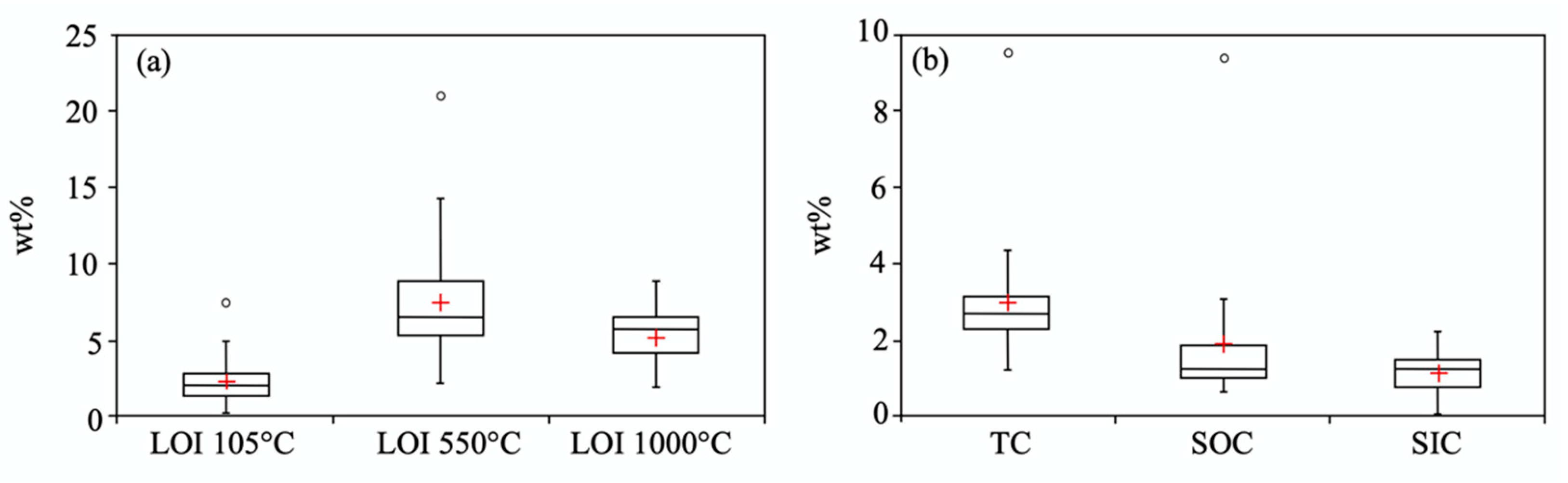
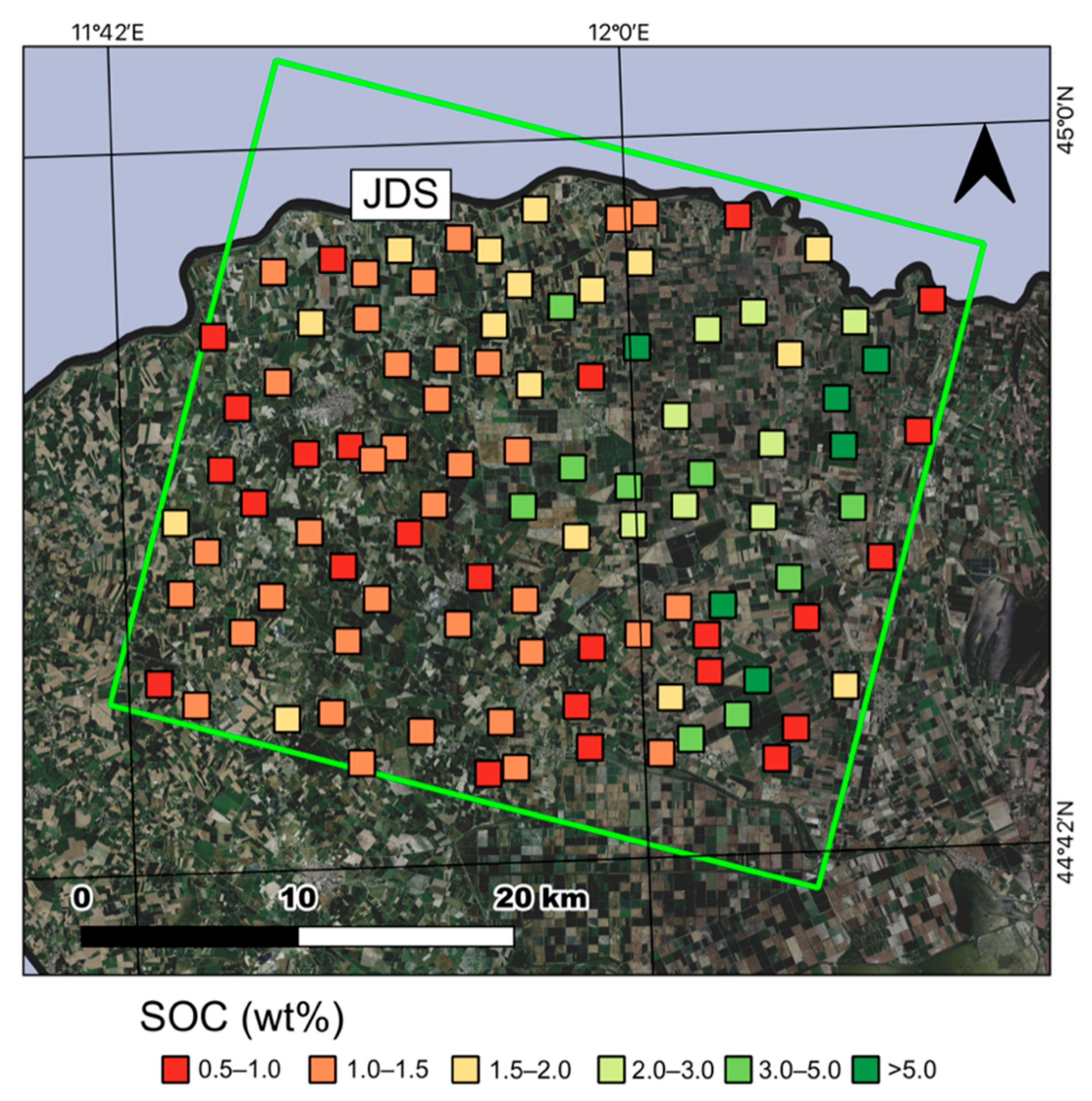
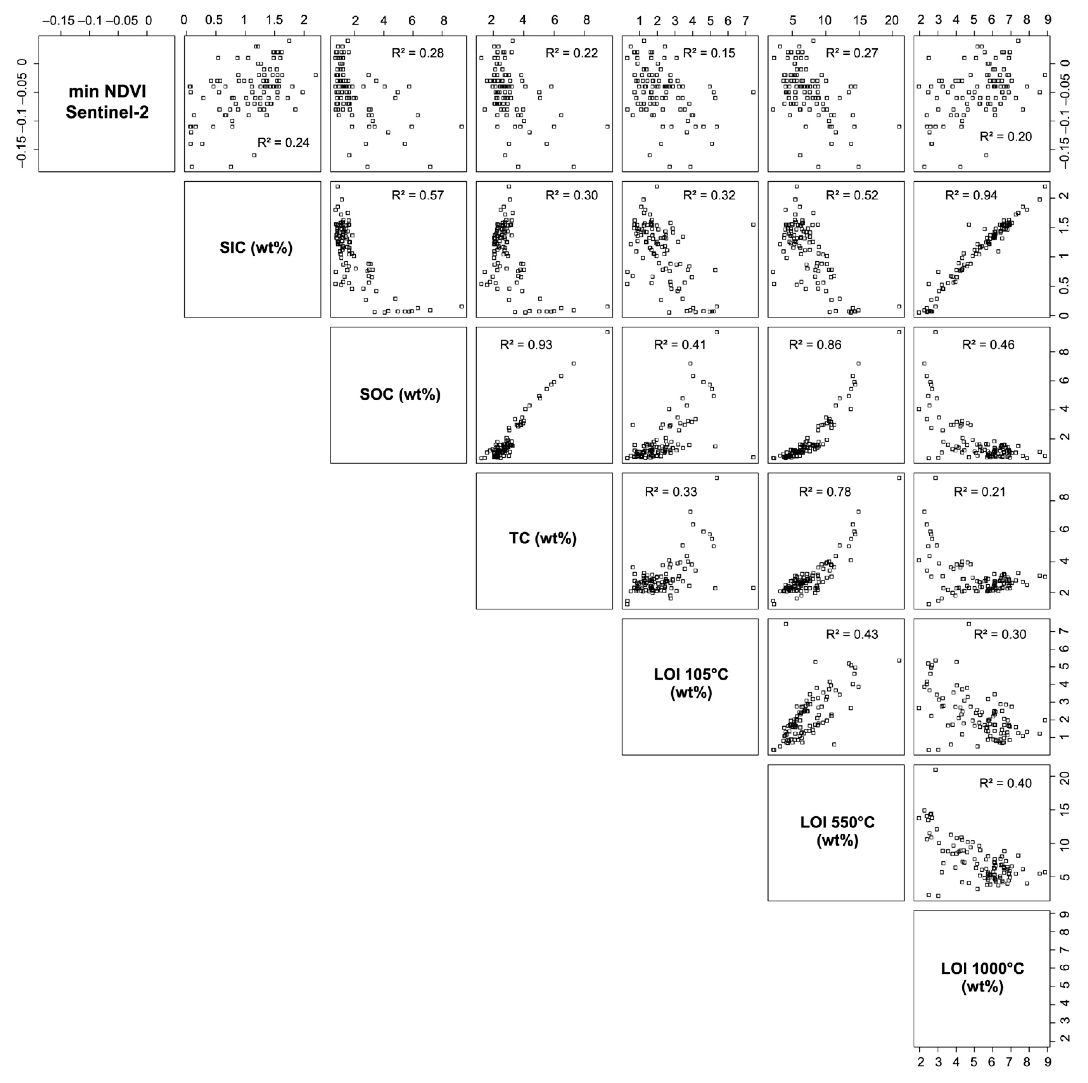
3.1. Geochemical Analyses

The distributions of the soil parameters analyzed in the JDS area are reported in Figure 2 and the complete analytical dataset is reported in Supplementary Table S2. According to the thermogravimetric analyses (Figure 2a), LOI 105 °C, which represents gypsum and hygroscopic water contents, varied between 0.30 wt% and 7.43 wt%, with an average of 2.23 wt%. LOI 550 °C, which is correlated with the SOM contents, had a large range varying from 2.14 wt% to 20.97 wt%, with an average of 7.40 wt%. The highest values of LOI 550 °C are indicative of the abundance of organic matter and they are typical of the soil samples collected in the northeastern part of Ferrara province, where peaty soils are present [38]. LOI 1000 °C, which represents carbonates and clay minerals, had a range between 1.96 wt% and 8.87 wt%, with an average of 5.25 wt% (Figure 2a). Low contents of carbonates in the soil samples were expected considering the scarce presence of carbonatitic lithology in the JDS area; therefore, LOI 1000 °C is probably mostly related to the presence of clay minerals. However, even if LOI 1000 °C totally represents the presence of clays, the clay mineral contents in the JDS soil samples are relatively low, posing a risk to SOM preservation in this area. In fact, clay minerals usually form aggregates in which the organic matter remains protected from microbial decomposition [39]. According to the C speciation analyses (Figure 2a), the TC varied between 1.21 wt% and 9.50 wt%, with an average of 2.96 wt%, the SOC values were between 0.68 wt% and 9.34 wt%, with an average of 1.87 wt%, and the SIC had a range between 0.05 wt% and 2.20 wt%, with an average of 1.09 wt%. The predominance of SOC in the JDS soil with respect to the SIC is indicative of the abundance of organic matter, typical of the peaty soil in this area. Figure 3 shows the distribution of SOC contents in JDS municipality and also evidences the strong variability in SOC contents in this area. The soil samples collected in the central and eastern parts of the area exhibit the highest SOC contents. These zones correspond to areas with peat soils [26], which are particularly enriched in SOM. Such soils resulted from the drainage wetland program started before World War II and ended in the 1970s, in which marshes and swamps were drained to develop new lands for agricultural purposes [33]. On the other hand, the western and most eastern parts of the JDS area, which do not host peat soils, show the lowest SOC contents. These areas are characterized by medium-fine or medium-textured soils [26]. Typically, soils with a medium-coarse texture have a scarce ability to sequester C with respect to their finer texture, as organic matter is easily accessible to microorganisms [39]. In addition, Brombin et al. [40] demonstrated that low contents of SOC are typical of agricultural fields located in the Padanian plain, including fields where farmers have adopted more sustainable management practices (e.g., minimum tillage and biological practices). This is due to the unfavorable pedoclimatic settings of the Padanian Plain like hot temperatures and droughts, which encourage the microbial activity that decomposes organic matter.

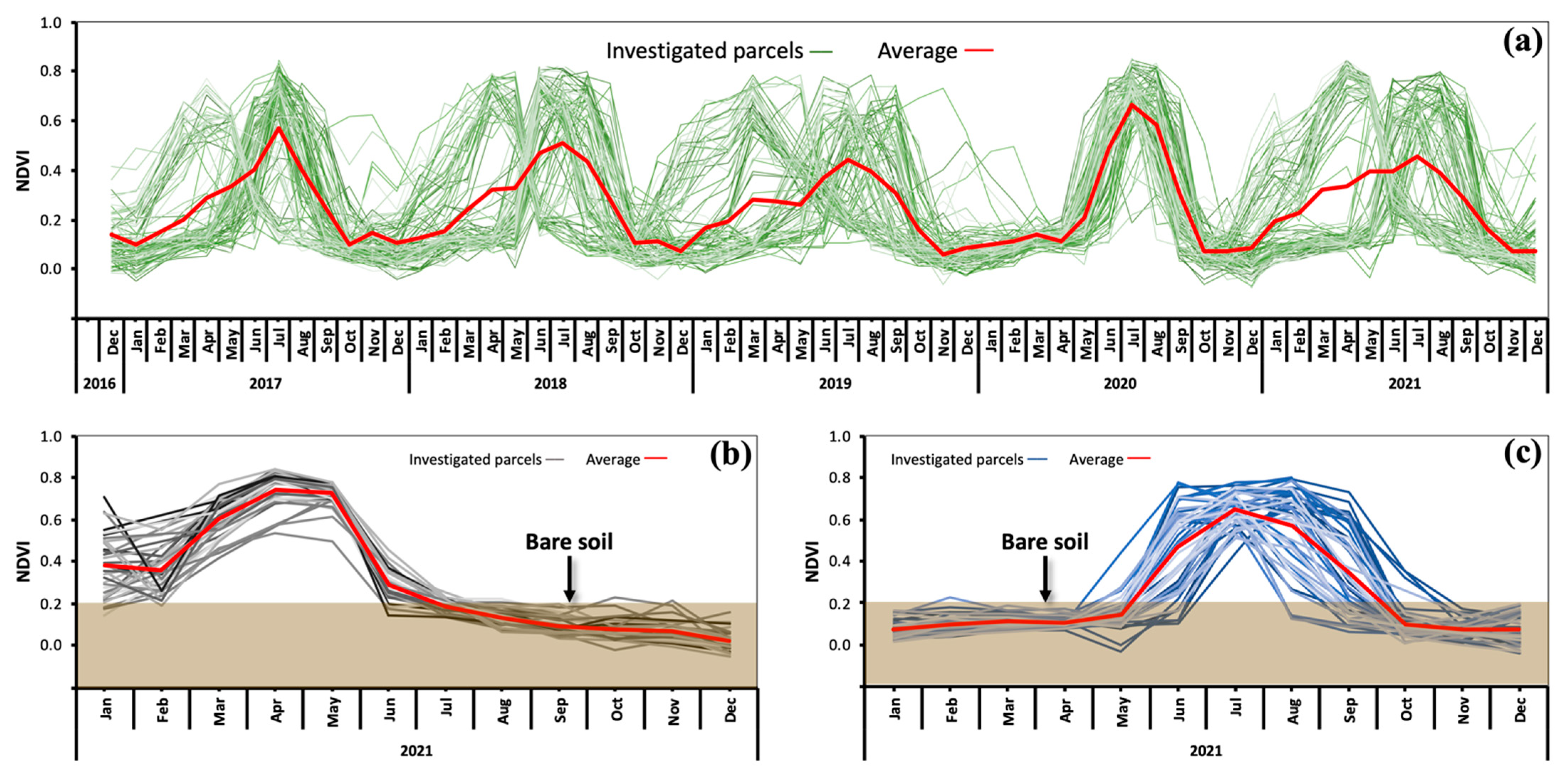
3.2. Time Series of the Sentinel-2 NDVI

For each investigated site, we downloaded a complete time series of the Sentinel-2 NDVI for the period of December 2016–December 2021 from the ADAM Platform. In general, in this period, the NDVI varied from −0.18 to 0.87, with an average of 0.28. Such values represent bare soil and dense vegetation conditions, respectively, as NDVI values lower than 0.3 are typical of soil with no cover vegetation; on the contrary, values higher than 0.7 are typical of strong green vegetation at the peak of growth. The time series thus made it possible to observe the phenological cycle [41,42] of each crop that covered the sampling sites.
The time series of the monthly averaged NDVI is reported in Figure 4a. Moreover, for the entire year of 2021, we recognized that 37 out of 100 sites were cultivated from before January to June with winter wheat (Figure 4b), while 47 sites were covered by vegetation from May to October with maize, soybean, and rice (Figure 4c). The remaining 16 sites were not cultivated or they displayed multiple phenological cycles (i.e., horticultural crops).
For each sampling site, the minimum NDVI values of Sentinel-2 are related to the soil conditions represented by the geochemical parameters. In Figure 5, the correlation plots show that the geochemical parameters related to carbon species are well correlated with the intrinsic characteristics of the soil. In particular, examples of good correlations exist between SOC and LOI 550 °C (R2 = 0.86), SOC and TC (R2 = 0.93), and SIC and LOI 1000 °C (R2 = 0.94). Despite the weak correlations, we can observe that the lower the NDVI index, the higher LOI 105 °C, LOI 550 °C, TC, and SOC (Figure 5). On the contrary, NDVI correlates positively with both LOI 1000 °C and SIC (Figure 5). Such conditions are probably imputable to the color of the bare soil. In particular, the high presence of black material, as occurs in the peaty soils of JDS or finer soils mainly composed of clay, is related to the lower NDVI values. On the other hand, soils with a high presence of carbonates and coarse material, which can favor SOM degradation and SOC depletions, are related to higher NDVI values.

3.3. Model Results

The performances of the models linking the soil spectra to the SOC content and the other soil properties are shown, in terms of R2, in Table 3. The R2 for SOC specifically was 0.64 for the OLS model but 0.49 for the neural network model. This suggests that the former is a more adequate modeling technique for this problem than the latter. It is important to note that, for both the OLS and ANN models, the FDR spectra perform better than the original spectra and that the models using the “optimal” inputs defined in Section 2.5.1 are an improvement over those that use the original bands. This implies that spectral features linked to SOC may indeed better emerge in the FDR spectra and that indicators obtained by combining pairs of bands may highlight soil properties even further.
Table 4 shows which input variables were significant in the OLS model for SOC. It is evident that among the “optimal” inputs, the spectral indices (NDI and DI) are significant, while the wavelengths are not. This is not surprising, as the indices were chosen based on their correlation with the SOC values.
Among the PRISMA bands, the most significant appear to be the 434 nm band for the FDR spectra and the 623 nm band for the original spectra.
The model for SOC yielded better performance than those for the other soil properties. Therefore, organic carbon appears to be easier to detect from soil spectra than inorganic carbon or other soil properties. Among the soil properties other than carbon, the models that performed best were those for SOM (LOI 550 °C) and the inorganic fraction (LOI 1000 °C), both with R2 above 0.5. The OLS models performed better than the ANN models for all the variables except SIC and the inorganic fraction. The best-performing OLS models were usually the ones using FDR spectra and “optimal” inputs, while the ANN models usually performed better with the original spectra. Our models performed worse than those employed in previous studies. Meng et al. [24], who performed a similar study, associated data of the GaoFen-5 hyperspectral satellite with 315 soil samples collected in an area of 80 × 80 Km2 in Northeast China and obtained R2 = 0.83 using FDR spectra and an ANN model. Mzid et al. [43] associated PRISMA data with 61 soil samples collected in two small study areas (up to 3 × 3 Km2) in Lazio and Basilicata (central–southern Italy), characterized by restricted SOC variability (0.2–2.1 wt%). The authors reached R2 = 0.85 using PLSR and Cubist regression on the original PRISMA spectra. Therefore, our results seem worse than those reported in the literature. However, it should be taken into account that the former study used a considerably larger dataset (>300 samples), while the latter operated over smaller study areas characterized by far lower carbon variability. On the contrary, the study area selected for this work is wider and characterized by greater soil and SOC variability due to the complex alluvial–deltaic environment and moreover due to the simultaneous presence of cultivated soils with and without peat soils, enriched in SOM. The flaws of PRISMA data are other reasons for the poor performance of our model. The geolocation error affecting the PRISMA pixels was particularly problematic. We chose to use L2C PRISMA products because we were aware that the SOC content could vary significantly on a scale smaller than the 30 m resolution of the PRISMA sensor. We thus needed to take multiple samples in the area covered by each pixel (see Section 2.3) to obtain the average properties that might correspond to the average soil spectrum captured in that pixel. Since the L2C product preserved the original observation geometry, whereas the L2D product did not, we therefore chose to use the former, albeit at the cost of using an image that was not geocoded to a specific geographic coordinate system. However, the L2C pixel geolocation was affected by an error that could exceed 30 m, making it complicated to match each sampling site with the correct PRISMA pixel. We had to carry this out visually, with the help of the 5 m panchromatic image. Our work was further complicated by the presence of a discrepancy between the hyperspectral and panchromatic images, as the corresponding pixels in the two images did not cover precisely the same area and the difference also sometimes exceeded 30 m.

4. Conclusions

This study attempted to develop a methodology that would use hyperspectral satellite data and geochemical analysis of in situ soil samples to predict soil organic carbon (SOC) content at Jolanda di Savoia (JDS), in Ferrara Province, which is characterized by extreme variability in soil types and composition. In fact, according to the geochemical analyses of soil samples collected in the study area, JDS shows SOC variability (0.7–9.3 wt%) due to the complexity of its alluvial–deltaic environment. The central and eastern parts of the study area exhibit the highest SOC contents, as they host peat soils enriched in SOM. On the contrary, the western and most eastern parts of the JDS area, are characterized by low SOC contents, as they are medium-fine or medium-textured soils, which are not able to protect the SOM from the depletion triggered by the climatic conditions and/or unsustainable agricultural practices. It is clear that in this context, an accessible digital map showing the distribution of SOC is fundamental for farmers and policymakers. In particular, global warming and climate change also due to agricultural impacts (e.g., CO2 released into the atmosphere due to the breakdown of organic matter compounds) are transforming environments and soil compositions (e.g., SOC baseline). Therefore, our study shows how predictions of geochemical maps in soils with high variability of SOC and other geochemical parameters are difficult to infer using spectral data. Nevertheless, our approach could be a useful tool to model such parameters in the near future which will impose more baselines related to environmental matrices.
In this area, our best-performing model for SOC prediction, obtained using ordinary least-squares (OLS) regression, reached a maximum R2 of 0.64, whereas a model based on a neural network reached only 0.49. This performance is not, in any case, sufficient to reliably predict the SOC content over the entire study area. In fact, in our case study, a large area such as JDS and with such high variables, the accuracy of SOC prediction is based not only on indices derived from remote sensing but also requires a higher population of in situ geochemical measurements and other accurate models. The production of an adequate model is made more difficult by the flaws in the PRISMA data, like geolocation errors and missing data, of which the experts should be warned to resolve the discrepancies. In summary, it is necessary to conduct further investigations (e.g., a greater number of soil surveys and geochemical analyses for the same area; new ad hoc spectral indexes for each soil type) to improve our local model prediction ability and provide a robust tool for soil carbon detection in areas characterized by extreme soil and organic carbon variability, such as Ferrara province. Updated soil mapping would be useful to estimate soil degradation and would constitute a helpful tool for policymakers and farmers to plan future sustainable land use and agricultural practices, especially in the areas hosting peat soils and/or susceptible to the effects of global warming. This is particularly urgent nowadays, considering the climatic issue with which our planet is dealing. In fact, besides the improvement of increased soil fertility, agricultural sustainable practices will play a significant role in the mitigation of climate change, sequestering C from the atmosphere and reducing greenhouse gas emissions.

Supplementary Materials

The following supporting information can be downloaded at: https://www.mdpi.com/article/10.3390/environments10100173/s1. Table S1: Parameters of the configuration of the ordinary least-squares (OLS), neural network (ANN), and significant variables of the OLS. Table S2: Dataset of the analyses of the total carbon (TC), soil organic carbon (SOC), soil inorganic carbon (SIC), loss on ignition at 105 °C (LOI 105 °C), loss on ignition at 550 °C (LOI 550 °C), and loss on ignition at 1000 °C (LOI 1000 °C). Supplementary folder: Codes for OLS and ANNs in R and Python, respectively.

Author Contributions

Conceptualization, G.B.; methodology, G.M.S., M.L., V.B. and G.B.; software, G.M.S. and M.L.; formal analysis, G.M.S. and G.B.; investigation, G.M.S., M.L., G.B. and S.N.; data curation, G.M.S., M.L., V.B. and G.B.; writing—original draft preparation, G.M.S., M.L., V.B. and G.B.; writing—review and editing, M.L., V.B., G.B., S.N. and C.N.; supervision, G.B. All authors have read and agreed to the published version of the manuscript.

Funding

This research received no external funding.

Data Availability Statement

The data presented in this study are available in the Supplementary Material of this article.

Acknowledgments

The authors give thanks to Flavio Fornasier of CREA laboratories of Gorizia for their support during the geochemical analyses. Finally, the authors thank the editorial office and two anonymous reviewers for their suggestions to improve the early version of the manuscript.

Conflicts of Interest

The authors declare no conflict of interest.

References

  1. National Research Council. Basic Research Opportunities in Earth Science; National Academy Press: Washington, DC, USA, 2001; p. 168. [Google Scholar]
  2. Xu, X.; Liu, W. The global distribution of Earth’s critical zone and its controlling factors. Geophys. Res. Lett. 2017, 44, 3201–3208. [Google Scholar] [CrossRef]
  3. Chorover, J.; Kretzschmar, R.; Garcia-Pichel, F.; Sparks, D.L. Soil biogeochemical processes within the critical zone. Elements 2007, 3, 321–326. [Google Scholar] [CrossRef]
  4. Bünemann, E.K.; Bongiorno, G.; Bai, Z.; Creamer, R.E.; De Deyn, G.; De Goede, R.; Fleskens, L.; Geissen, V.; Kuyper, T.W.; Mäder, P.; et al. Soil Quality—A Critical Review. Soil. Biol. Biochem. 2018, 120, 105–125. [Google Scholar] [CrossRef]
  5. Hoffland, E.; Kuyper, T.W.; Comans, R.N.J.; Creamer, R.E. Eco-functionality of organic matter in soils. Plant Soil 2020, 455, 1–22. [Google Scholar] [CrossRef]
  6. Deb, S.; Bhadoria, P.B.S.; Mandal, B.; Rakshit, A.; Singh, H.B. Soil organic carbon: Towards better soil health, productivity and climate change mitigation. Clim. Chang. Environ. Sustain. 2015, 3, 26. [Google Scholar] [CrossRef]
  7. Minasny, B.; McBratney, A.B.; Malone, B.P.; Wheeler, I. Digital mapping of soil carbon. In Advances in Agronomy; Elsevier: Amsterdam, The Netherlands, 2013; Volume 118, pp. 1–47. [Google Scholar]
  8. Scharlemann, J.P.; Tanner, E.V.; Hiederer, R.; Kapos, V. Global soil carbon: Understanding and managing the largest terrestrial carbon pool. Carbon Manag. 2014, 5, 81–91. [Google Scholar] [CrossRef]
  9. Sanderman, J.; Hengl, T.; Fiske, G.J. Soil carbon debt of 12,000 years of human land use. Proc. Natl. Acad. Sci. USA 2017, 114, 9575–9580. [Google Scholar] [CrossRef]
  10. Keskin, H.; Grunwald, S.; Harris, W.G. digital mapping of soil carbon fractions with machine learning. Geoderma 2019, 339, 40–58. [Google Scholar] [CrossRef]
  11. Sothe, C.; Gonsamo, A.; Arabian, J.; Kurz, W.A.; Finkelstein, S.A.; Snider, J. Large soil carbon storage in terrestrial ecosystems of Canada. Glob. Biogeochem. Cycles 2022, 36, e2021GB007213. [Google Scholar] [CrossRef]
  12. Angelopoulou, T.; Tziolas, N.; Balafoutis, A.; Zalidis, G.; Bochtis, D. Remote sensing techniques for soil organic carbon estimation: A review. Remote Sens. 2019, 11, 676. [Google Scholar] [CrossRef]
  13. Batjes, N.H. Harmonized soil profile data for applications at global and continental scales: Updates to the WISE database. Soil Use Manag. 2009, 25, 124–127. [Google Scholar] [CrossRef]
  14. Tóth, G.; Jones, A.; Montanarella, L. The LUCAS topsoil database and derived information on the regional variability of cropland topsoil properties in the European Union. Environ. Monit. Assess. 2013, 185, 7409–7425. [Google Scholar] [CrossRef]
  15. Wills, S.; Loecke, T.; Sequeira, C.; Teachman, G.; Grunwald, S.; West, L.T. Overview of the U.S. Rapid Carbon Assessment Project: Sampling design, initial summary and uncertainty estimates. In Soil Carbon; Springer International Publishing: Cham, Switzerland, 2014; pp. 95–104. [Google Scholar]
  16. Viscarra Rossel, R.; Behrens, T.; Ben-Dor, E.; Brown, D.; Demattê, J.; Shepherd, K.; Shi, Z.; Stenberg, B.; Stevens, A.; Adamchuk, V.; et al. A global spectral library to characterize the world’s soil. Earth-Sci. Rev. 2016, 155, 198–230. [Google Scholar] [CrossRef]
  17. Stevens, A.; Nocita, M.; Tóth, G.; Montanarella, L.; van Wesemael, B. Prediction of soil organic carbon at the European scale by visible and near infrared reflectance spectroscopy. PLoS ONE 2013, 8, e66409. [Google Scholar] [CrossRef]
  18. Biney, J.K.M.; Saberioon, M.; Borůvka, L.; Houška, J.; Vašát, R.; Chapman Agyeman, P.; Coblinski, J.A.; Klement, A. Exploring the suitability of UAS-based multispectral images for estimating soil organic carbon: Comparison with proximal soil sensing and spaceborne imagery. Remote Sens. 2021, 13, 308. [Google Scholar] [CrossRef]
  19. Vaudour, E.; Gholizadeh, A.; Castaldi, F.; Saberioon, M.; Borůvka, L.; Urbina-Salazar, D.; Fouad, Y.; Arrouays, D.; Richer-de-Forges, A.C.; Biney, J.; et al. Satellite imagery to map topsoil organic carbon content over cultivated areas: An overview. Remote Sens. 2022, 14, 2917. [Google Scholar] [CrossRef]
  20. Li, S.; Viscarra Rossel, R.A.; Webster, R. The cost-effectiveness of reflectance spectroscopy for estimating soil organic carbon. Eur. J. Soil Sci. 2022, 73, e13202. [Google Scholar] [CrossRef]
  21. Ben-Dor, E.; Chabrillat, S.; Demattê, J.A.M.; Taylor, G.R.; Hill, J.; Whiting, M.L.; Sommer, S. Using imaging spectroscopy to study soil properties. Remote Sens. Environ. 2009, 113, S38–S55. [Google Scholar] [CrossRef]
  22. Nocita, M.; Stevens, A.; Van Wesemael, B.; Aitkenhead, M.; Bachmann, M.; Barthès, B.; Ben Dor, E.; Brown, D.J.; Clairotte, M.; Csorba, A.; et al. Soil spectroscopy: An alternative to wet chemistry for soil monitoring. In Advances in Agronomy; Academic Press: Cambridge, MA, USA, 2015; Volume 132, pp. 139–159. [Google Scholar] [CrossRef]
  23. Wang, S.; Guan, K.; Zhang, C.; Lee, D.; Margenot, A.J.; Ge, Y.; Peng, J.; Zhou, W.; Zhou, Q.; Huang, Y. Using soil library hyperspectral reflectance and machine learning to predict soil organic carbon: Assessing potential of airborne and spaceborne optical soil sensing. Remote Sens. Environ. 2022, 271, 112914. [Google Scholar] [CrossRef]
  24. Meng, X.; Bao, Y.; Liu, J.; Liu, H.; Zhang, X.; Zhang, Y.; Wang, P.; Tang, H.; Kong, F. Regional soil organic carbon prediction model based on a discrete wavelet analysis of hyperspectral satellite data. Int. J. Appl. Earth Obs. Geoinf. 2020, 89, 102111. [Google Scholar] [CrossRef]
  25. Pignatti, S.; Palombo, A.; Pascucci, S.; Romano, F.; Santini, F.; Simoniello, T.; Umberto, A.; Vincenzo, C.; Acito, N.; Diani, M.; et al. The PRISMA hyperspectral mission: Science activities and opportunities for agriculture and land monitoring. In Proceedings of the 2013 IEEE International Geoscience and Remote Sensing Symposium—IGARSS, Melbourne, Australia, 21–26 July 2013; pp. 4558–4561. [Google Scholar]
  26. Colombani, N.; Salemi, E.; Mastrocicco, M.; Castaldelli, G. Groundwater nitrogen speciation in intensively cultivated lowland areas. In Advances in the Research of Aquatic Environment; Springer Berlin Heidelberg: Berlin/Heidelberg, Germany, 2011; pp. 291–298. [Google Scholar]
  27. Di Giuseppe, D.; Bianchini, G.; Vittori Antisari, L.; Martucci, A.; Natali, C.; Beccaluva, L. Geochemical characterization and biomonitoring of reclaimed soils in the Po River delta (Northern Italy): Implications for the agricultural activities. Environ. Monit. Assess. 2014, 186, 2925–2940. [Google Scholar] [CrossRef]
  28. Amorosi, A.; Centineo, M.C.; Dinelli, E.; Lucchini, F.; Tateo, F. Geochemical and mineralogical variations as indicators of provenance changes in Late Quaternary deposits of SE Po Plain. Sediment. Geol. 2002, 151, 273–292. [Google Scholar] [CrossRef]
  29. Mastrocicco, M.; Colombani, N.; Salemi, E.; Castaldelli, G. Numerical assessment of effective evapotranspiration from maize plots to estimate groundwater recharge in lowlands. Agric. Water Manag. 2010, 97, 1389–1398. [Google Scholar] [CrossRef]
  30. Bianchini, G.; Cremonini, S.; Di Giuseppe, D.; Gabusi, R.; Marchesini, M.; Vianello, G.; Vittori Antisari, L. Late Holocene palaeo-environmental reconstruction and human settlement in the Eastern Po Plain (Northern Italy). Catena 2019, 176, 324–335. [Google Scholar] [CrossRef]
  31. Bianchini, G.; Di Giuseppe, D.; Natali, C.; Beccaluva, L. Ophiolite inheritance in the Po Plain sediments: Insights on heavy metals distribution and risk assessment. Ofioliti 2013, 38, 1–14. [Google Scholar] [CrossRef]
  32. Simeoni, U.; Corbau, C. A Review of the delta Po evolution (Italy) related to climatic changes and human impacts. Geomorphology 2009, 107, 64–71. [Google Scholar] [CrossRef]
  33. Targetti, S.; Raggi, M.; Zavalloni, M.; Viaggi, D. Perceived benefits from reclaimed rural landscapes: Evidence from the lowlands of the Po River delta, Italy. Ecosyst. Serv. 2021, 49, 101288. [Google Scholar] [CrossRef]
  34. Guarini, R.; Loizzo, R.; Longo, F.; Mari, S.; Scopa, T.; Varacalli, G. Overview of the PRISMA space and ground segment and its hyperspectral products. In Proceedings of the 2017 IEEE International Geoscience and Remote Sensing Symposium (IGARSS), Fort Worth, TX, USA, 23–28 July 2017; pp. 431–434. [Google Scholar]
  35. Pepe, M.; Pompilio, L.; Gioli, B.; Busetto, L.; Boschetti, M. Detection and classification of non-photosynthetic vegetation from PRISMA hyperspectral data in croplands. Remote Sens. 2020, 12, 3903. [Google Scholar] [CrossRef]
  36. Dean, W.E. Determination of carbonate and organic matter in calcareous sediments and sedimentary rocks by loss on ignition—Comparison with other methods. J. Sediment. Res. 1974, 44, 242–248. [Google Scholar]
  37. Zethof, J.H.T.; Leue, M.; Vogel, C.; Stoner, S.W.; Kalbitz, K. Identifying and quantifying geogenic organic carbon in soils—The case of graphite. Soil 2019, 5, 383–398. [Google Scholar] [CrossRef]
  38. Natali, C.; Bianchini, G.; Cremonini, S.; Salani, G.M.; Vianello, G.; Brombin, V.; Ferrari, M.; Vittori Antisari, L. Peat soil burning in the Mezzano Lowland (Po Plain, Italy): Triggering mechanisms and environmental consequences. Geohealth 2021, 5, e2021GH000444. [Google Scholar] [CrossRef]
  39. Sarkar, B.; Singh, M.; Mandal, S.; Churchman, G.J.; Bolan, N.S. Clay Minerals—Organic Matter Interactions in Relation to Carbon Stabilization in Soils. In The Future of Soil Carbon; Academic Press: Cambridge, MA, USA, 2018; pp. 71–86. [Google Scholar]
  40. Brombin, V.; Mistri, E.; Feudis, M.D.; Forti, C.; Salani, G.M.; Natali, C.; Falsone, G.; Vittori Antisari, L.; Bianchini, G. Soil carbon investigation in three pedoclimatic and agronomic settings of Northern Italy. Sustainability 2020, 12, 539. [Google Scholar] [CrossRef]
  41. Griffith, J.A.; Martinko, E.A.; Whistler, J.L.; Price, K.P. Interrelationships among landscapes, NDVI, and stream water quality in the U.S. Central Plains. Ecol. Appl. 2002, 12, 1702–1718. [Google Scholar] [CrossRef]
  42. Zhong, C.; Wang, C.; Wu, C. MODIS-based fractional crop mapping in the U.S. Midwest with spatially constrained phenological mixture analysis. Remote Sens. 2015, 7, 512–529. [Google Scholar] [CrossRef]
  43. Mzid, N.; Castaldi, F.; Tolomio, M.; Pascucci, S.; Casa, R.; Pignatti, S. Evaluation of agricultural bare soil properties retrieval from Landsat 8, Sentinel-2 and PRISMA satellite data. Remote Sens. 2022, 14, 714. [Google Scholar] [CrossRef]
Figure 1. (a) Location of the sampling sites within the study area Jolanda di Savoia (JDS; represented using the border, in green, of the 30 × 30 Km2 area covered by the PRISMA image) in Ferrara province, Emilia-Romagna region (Northern Italy), and (b) in each location, a composite sample was collected, mixing five aliquots of soil within a square (30 × 30 m2) probed at a depth of 0–15 cm.
Environments 10 00173 g001
Figure 2. Box and whisker distribution plots of the results of the analyzed JDS topsoils: (a) thermo-gravimetric analyses (i.e., LOI 105 °C, LOI 550 °C, and LOI 1000 °C) and (b) elemental carbon speciation (i.e., TC, SOC, and SIC). Average (red cross) and median (black line) values are also reported.
Environments 10 00173 g002
Figure 3. The SOC contents in the 100 soil samples collected in the JDS municipality measured through geochemical analysis.
Environments 10 00173 g003
Figure 4. (a) Sentinel-2 NDVI time series of the 100 sampling sites for the period December 2016–December 2021; (b) the Sentinel-2 NDVI time series in 2021 of 37 sampling sites show a phenological cycle typical of winter wheat (bare soil conditions are under the brownfield); and (c) Sentinel-2 NDVI time series in 2021 of 47 sampling sites that show a phenological cycle typical of summer cultivars as maize soybean and rice (bare soil conditions are under the brownfield). The averaged time series are represented by a red curve.
Environments 10 00173 g004
Figure 5. Correlation plots among the minimum calculated Sentinel-2 NDVI (period: December 2016–December 2021), SIC, SOC, TC, LOI 105 °C, LOI 550 °C, and LOI 1000 °C.
Environments 10 00173 g005
Table 1. Number of sampling locations (out of 100) for which, in each date corresponding to the JDS PRISMA images, the Sentinel-2 NDVI value is smaller than the bare soil upper limit. The numbers do not take into consideration the possibility that some of the sampling locations might be outside the area imaged by PRISMA on each date, which is never precisely the same.
PRISMA DateSentinel-2 DateNDVI
<0.2<0.3
21 October 201921 October 20199396
7 April 20208 April 202099100
17 May 202018 May 20208099
23 May 202023 May 20204569
26 June 202027 June 202059
31 July 20201 August 202015
16 September 202015 September 20205268
14 February 202114 February 2021712
24 April 202123 April 20216876
23 May 202123 May 20214661
4 June 20214 June 202166
11 September 202110 September 20215465
Table 2. PRISMA bands that were excluded from the data. The bands were excluded due to atmospheric absorption (i.e., they were not within an atmospheric window) or because they were invalid (i.e., all data were missing and no central wavelength was indicated in the metadata). Two bands, finally, were excluded because half the image was missing from the corresponding data slice.
Spectral RegionBand NumberCentral Wavelength (nm)Reason for ExclusionOptimal Inputs
Bands
VNIR1–3N/AInvalid bands0.598
VNIR66402.4402Half the image missing0.513
SWIR1–32496.874–2483.5906Atmospheric absorption0.336
SWIR72–861949.639–1812.8206Atmospheric absorption
SWIR126–1321416.3103–1349.599Atmospheric absorption0.405
SWIR171942.9579Half the image missing0.564
SWIR172–173N/AInvalid bands0.450
Table 3. R2 values obtained from the cross-validation of the OLS and ANN models for the various soil properties using the FDR and original spectra. For the OLS spectra, both the “optimal” inputs computed in Section 2.5.1 and the original spectral bands were used, while only the former inputs were used for the ANN.
Geochemical ParameterOLS RegressionNeural Network
FDR SpectraOriginal SpectraFDR SpectraOriginal Spectra
BandsOptimal InputsBandsOptimal InputsOptimal InputsOptimal Inputs
SOC0.5460.6410.5600.5980.4900.441
SIC0.4670.4730.4000.5130.4760.523
TC0.3280.5420.3430.3360.1740.203
LOI 105 °C 0.3730.3720.3720.4050.1610.223
LOI 550 °C 0.4920.5540.5440.5640.4200.463
LOI 1000 °C0.5060.5240.4630.4500.4320.535
Table 4. Significant variables in the OLS models for SOC. The PRISMA bands are indicated using the central wavelength preceded by the letter ‘W’. The bands used to compute the NDI and DI indices are also indicated. For each variable, the coefficient, its error, and its p-value are indicated.
First DerivativeOriginal
VariableCoeffErrorp-ValueVariableCoeffErrorp-Value
Bands(Intercept)2.48740.1996<2 × 10⁻¹⁶(Intercept)2.43010.2412<2 × 10⁻¹⁶
W411−532.181273.02370.0543W41111.53696.69230.088
W434−3114.71610.71111.76 × 10−6W623−18.50793.31482.23 × 10−7
W1501612.3953253.13390.0175W1078−3.87622.45290.117
W21981059.413637.09330.0997W24563.86422.67640.152
W2283711.4486424.71820.0972
Optimal
values
(Intercept)2.14420.1763<2 × 10⁻¹⁶(Intercept)2.39810.2256<2 × 10⁻¹⁶
NDI (W596, W538)1.43790.49350.00443W1595−2.9851.80330.101
DI (W2143, W426)2064.025278.50084.68 × 10−11DI (W434, W463)121.071822.09373.36 × 10−7
Disclaimer/Publisher’s Note: The statements, opinions and data contained in all publications are solely those of the individual author(s) and contributor(s) and not of MDPI and/or the editor(s). MDPI and/or the editor(s) disclaim responsibility for any injury to people or property resulting from any ideas, methods, instructions or products referred to in the content.

