Coseismic Ground Deformation Reproduced through Numerical Modeling: A Parameter Sensitivity Analysis

 ,
,
Abstract
1. Introduction
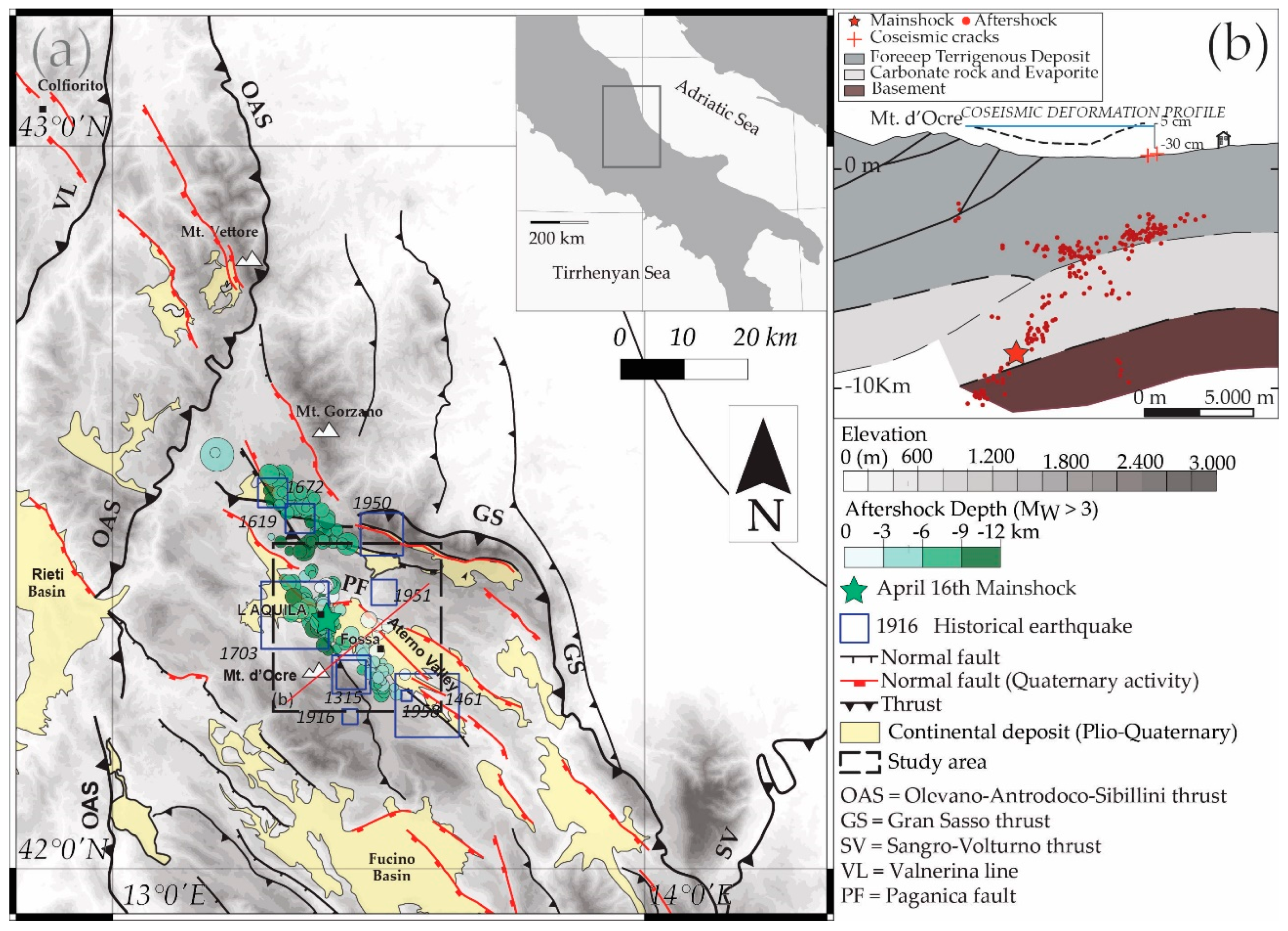
1.1. Study Area
1.2. L’Aquila Seismic Sequence
2. Surface and Subsurface Data
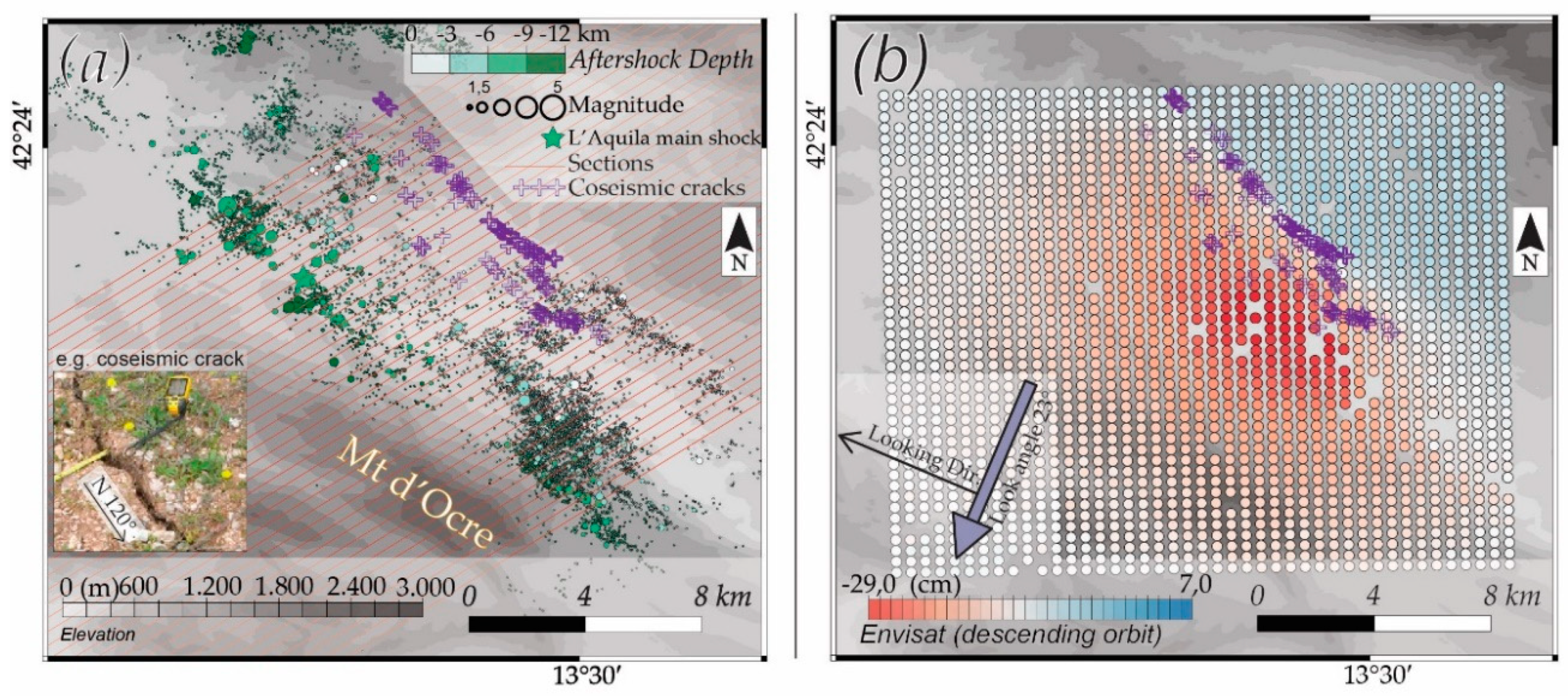
2.1. Surface Data
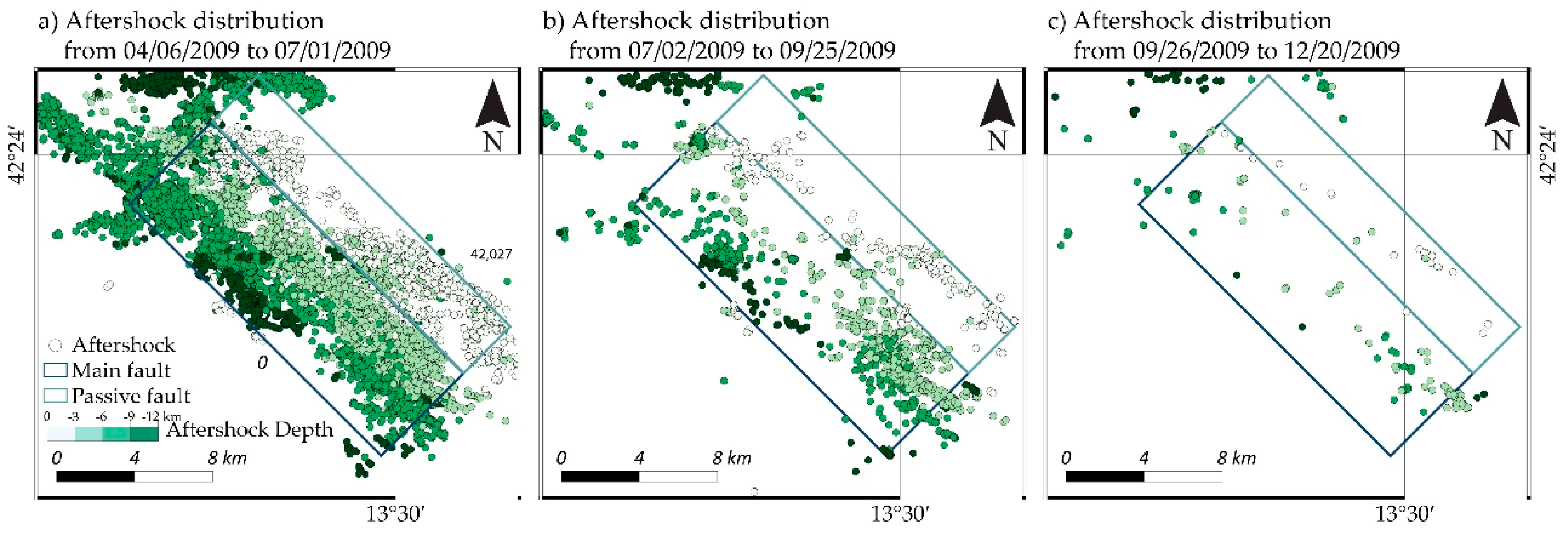
2.2. Aftershock Data
3. Methodology
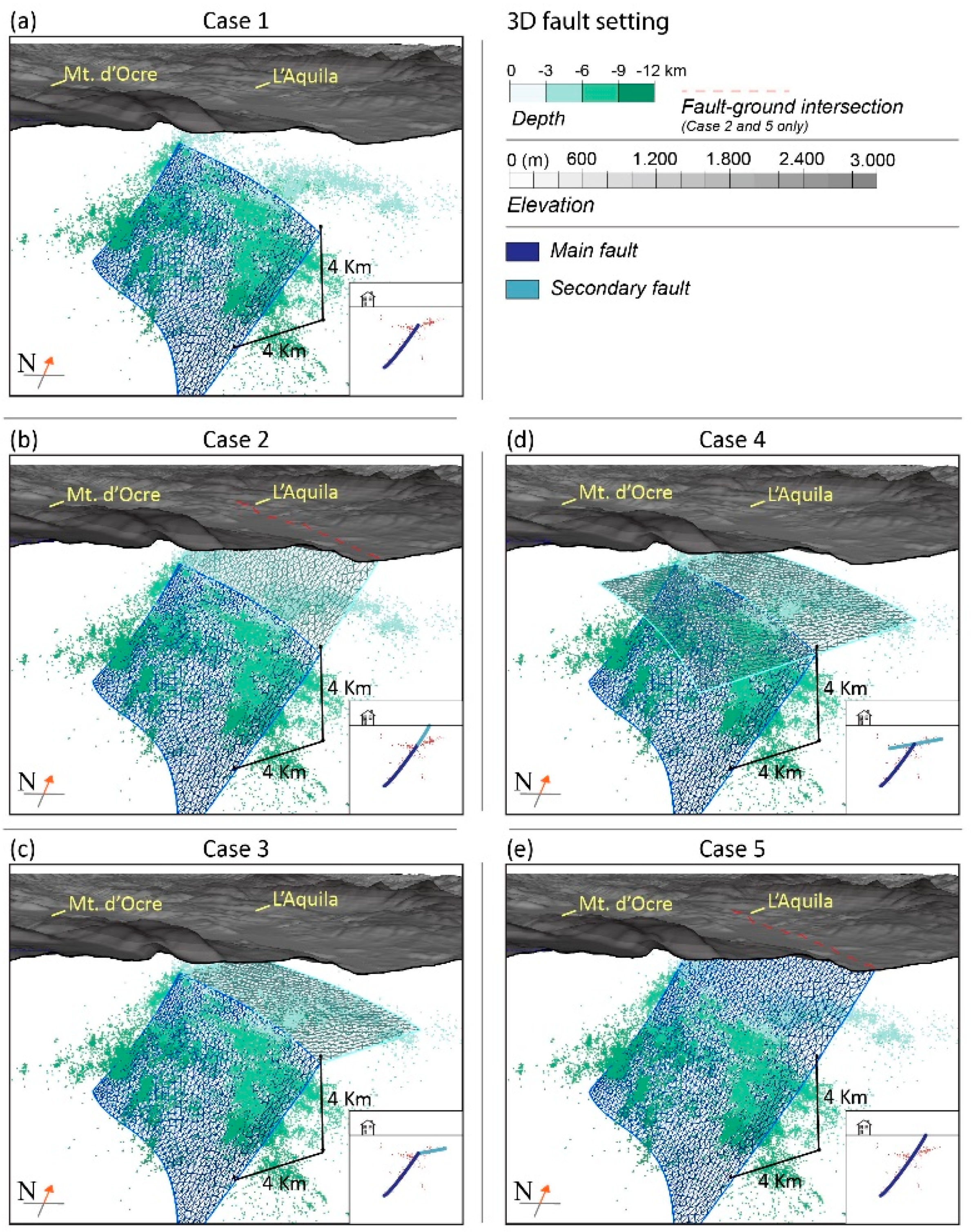
3.1. Fault Construction
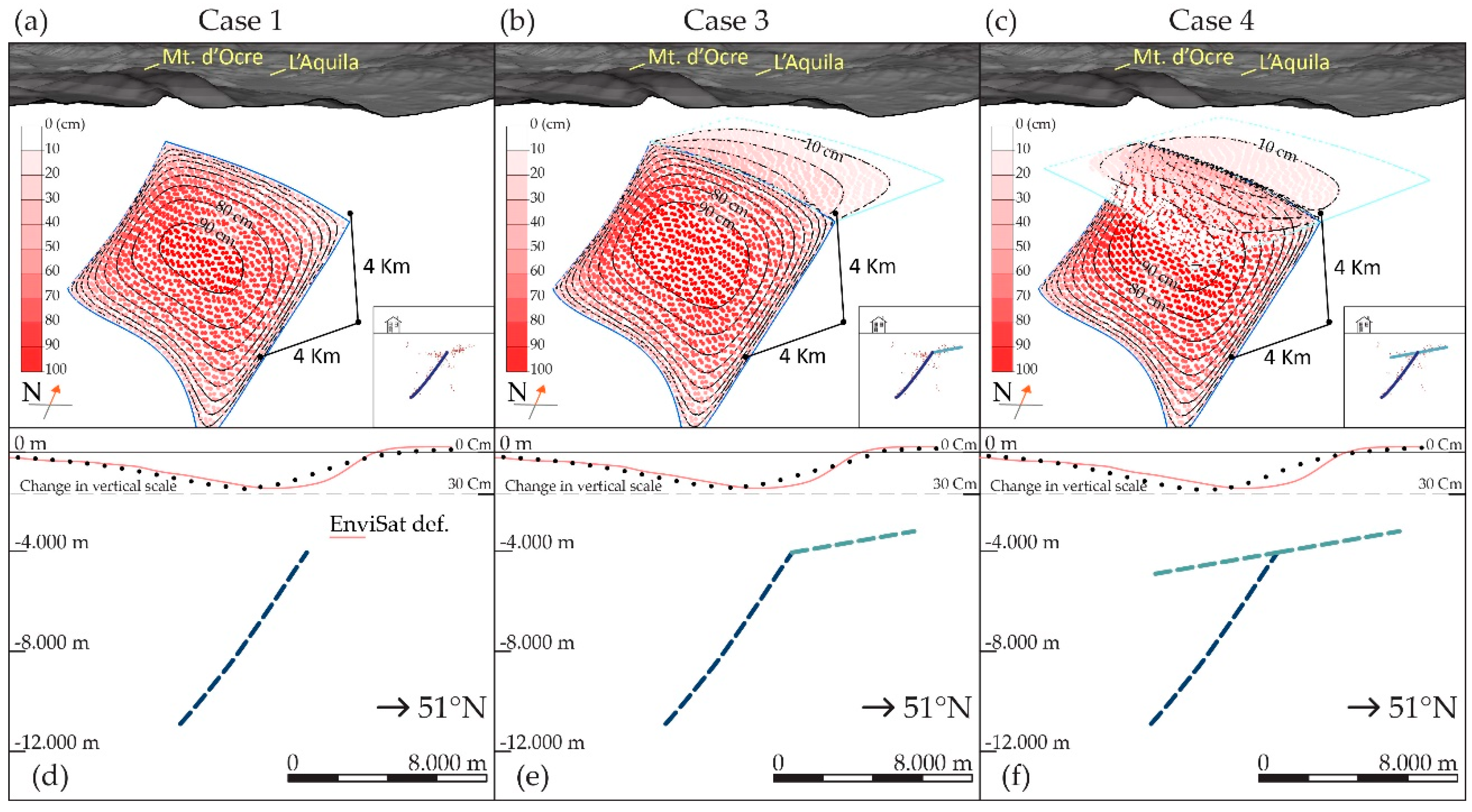
- Case 1 considers only the main blind normal fault extending from 3 to 11 km of depth;
- Case 2 includes the main fault and its prolongation up to the coseismic cracks mapped by Boncio et al. [12]. This model explores the possibility that coseismic slip along the main fault gives passive deformations along the third fault;
- Case 4 considers the main fault and the entire shallower low angle fault. This case follows reconstructions by Bonini et al. [16] that suggest a complete extensional reactivation of the thrust both in the hanging wall and in the footwall of the main fault;
- Case 5 is geometrically coincident with Case 2, but here the plane connected to the surface is not passively activated but it is part of the main fault plane reaching the surface. In this case we follow the conceptual model proposed by [14] where the main normal fault reaches the surface and the coseismic ground cracks are directly connected with the fault responsible for the L’Aquila earthquake.
3.2. Numerical Models
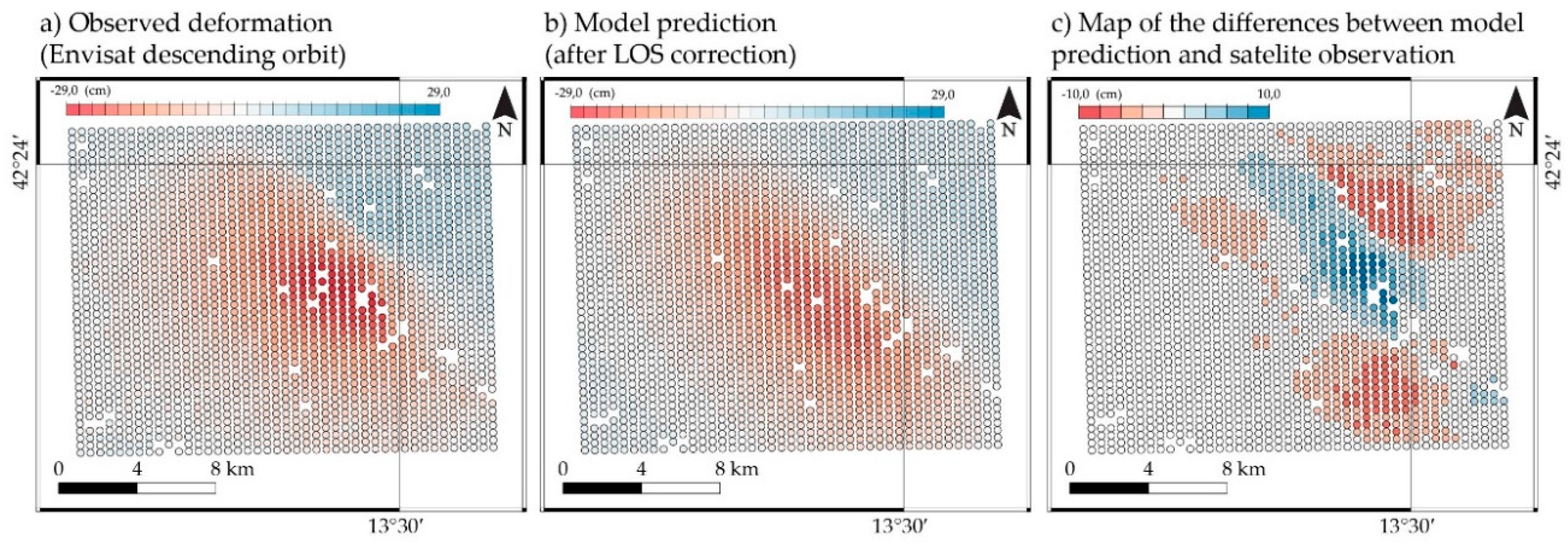
3.3. Line of Sight (LOS) Correction
4. Results
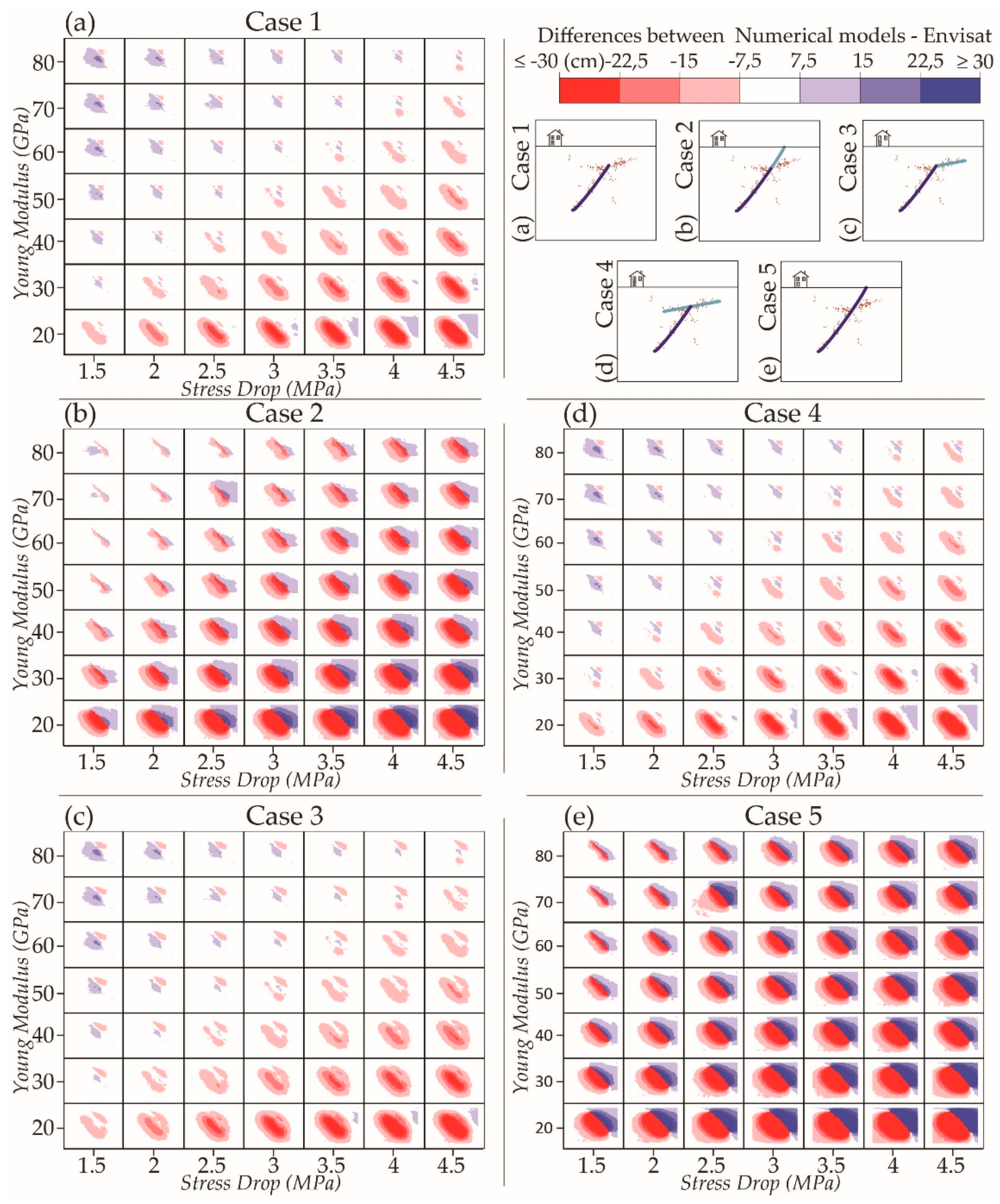
4.1. Residual Difference Maps
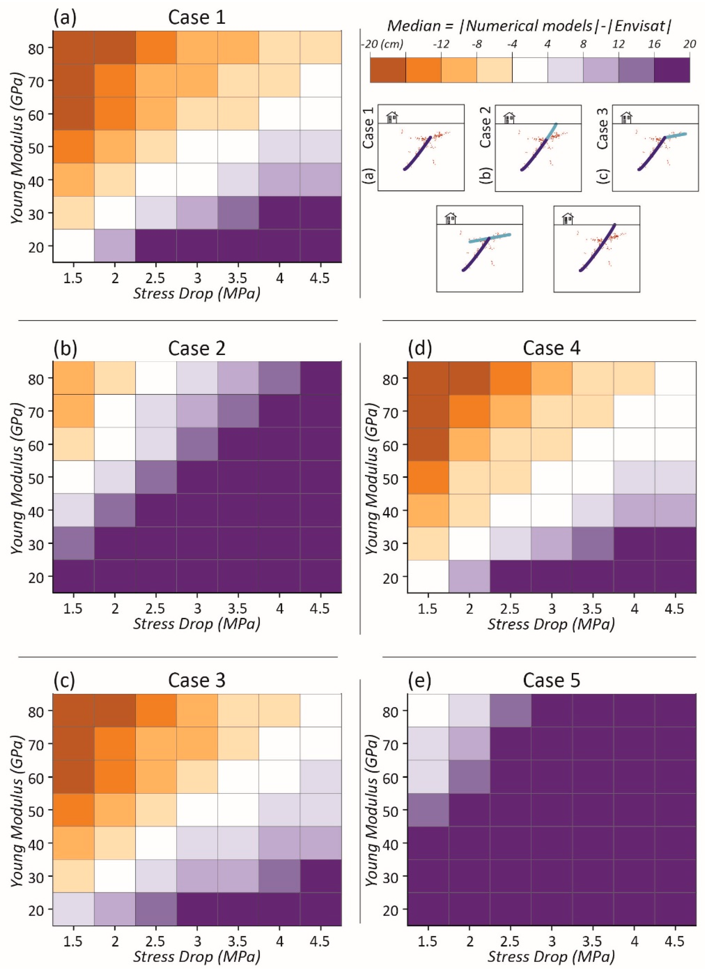
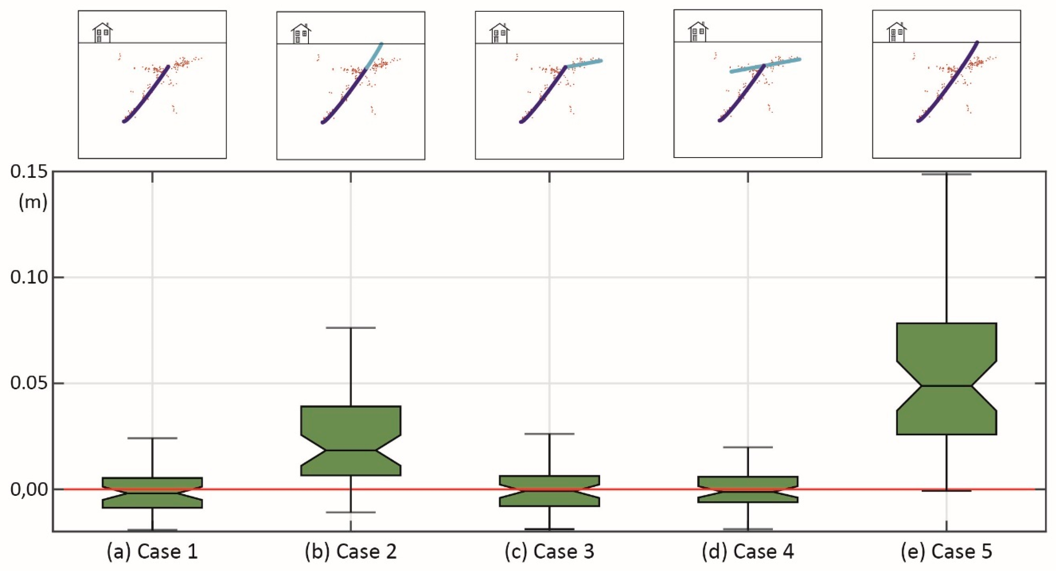
4.2. Median Net Difference
5. Discussion
6. Conclusions
Supplementary Materials
Author Contributions
Funding
Acknowledgments
Conflicts of Interest
References
- Massonnet, D.; Rossi, M.; Carmona, C.; Adragna, F.; Peltzer, G.; Feigl, K.; Rabaute, T. The displacement field of the Landers earthquake mapped by radar interferometry. Nature 1993, 364, 138–142. [Google Scholar] [CrossRef]
- Atzori, S.; Hunstad, I.; Chini, M.; Salvi, S.; Tolomei, C.; Bignami, C.; Stramondo, S.; Trasatti, E.; Antonioli, A.; Boschi, E. Finite fault inversion of DInSAR coseismic displacement of the 2009 L’Aquila earthquake (central Italy). Geophys. Res. Lett. 2009, 36. [Google Scholar] [CrossRef]
- Chini, M.; Atzori, S.; Trasatti, E.; Bignami, C.; Kyriakopoulos, C.; Tolomei, C.; Stramondo, S. The May 12, 2008, (Mw 7.9) Sichuan Earthquake (China): Multiframe ALOS-PALSAR DInSAR analysis of coseismic deformation. IEEE Geosci. Remote Sens. Lett. 2010, 7, 266–270. [Google Scholar] [CrossRef]
- Stramondo, S.; Cinti, F.R.; Dragoni, M.; Salvi, S.; Santini, S. The August 17, 1999 Izmit, Turkey, earthquake: Slip distribution from dislocation modeling of DInSAR and surface offset. Ann. Geophys. 2002, 45, 527–536. [Google Scholar]
- Walters, R.J.; Elliott, J.R.; D’Agostino, N.; England, P.C.; Hunstad, I.; Jackson, J.A.; Parsons, B.; Phillips, R.J.; Roberts Edinburgh, G. The 2009 L’Aquila earthquake (central Italy): A source mechanism and implications for seismic hazard. Geophys. Res. Lett. 2009, 36, L15305. [Google Scholar] [CrossRef]
- Wang, X.; Liu, G.; Yu, B.; Dai, K.; Zhang, R.; Chen, Q.; Li, Z. 3D coseismic deformations and source parameters of the 2010 Yushu earthquake (China) inferred from DInSAR and multiple-aperture InSAR measurements. Remote Sens. Environ. 2014, 152, 174–189. [Google Scholar] [CrossRef]
- Trasatti, E.; Kyriakopoulos, C.; Chini, M. Finite element inversion of DInSAR data from the Mw 6.3 L’Aquila earthquake, 2009 (Italy). Geophys. Res. Lett. 2011, 38, L08306. [Google Scholar] [CrossRef]
- Rovida, A.; Locati, M.; Camassi, R.; Lolli, B.; Gasperini, P. CPTI15, the 2015 Version of the Parametric Catalogue of Italian Earthquakes; Istituto Nazionale di Geofisica e Vulcanologia: Rome, Italy, 2016; pp. 1–33. [Google Scholar]
- Valoroso, L.; Chiaraluce, L.; Piccinini, D.; Di Stefano, R.; Schaff, D.; Waldhauser, F. Radiography of a normal fault system by 64,000 high-precision earthquake locations: The 2009 L’Aquila (central Italy) case study. J. Geophys. Res. Solid Earth 2013, 118, 1156–1176. [Google Scholar] [CrossRef]
- Scognamiglio, L.; Tinti, E.; Michelini, A.; Dreger, D.S.; Cirella, A.; Cocco, M.; Mazza, S.; Piatanesi, A. Fast Determination of Moment Tensors and Rupture History: What Has Been Learned from the 6 April 2009 L’Aquila Earthquake Sequence. Seismol. Res. Lett. 2010, 81, 892–906. [Google Scholar] [CrossRef]
- Serpelloni, E.; Anderlini, L.; Belardinelli, M.E. Fault geometry, coseismic-slip distribution and Coulomb stress change associated with the 2009 April 6, Mw 6.3, L’Aquila earthquake from inversion of GPS displacements. Geophys. J. Int. 2012, 188, 473–489. [Google Scholar] [CrossRef]
- Boncio, P.; Pizzi, A.; Brozzetti, F.; Pomposo, G.; Lavecchia, G.; Di Naccio, D.; Ferrarini, F. Coseismic ground deformation of the 6 April 2009 L’Aquila earthquake (central Italy, Mw6.3). Geophys. Res. Lett. 2010, 37, L06308. [Google Scholar] [CrossRef]
- Vannoli, P.; Burrato, P.; Fracassi, U.; Valensise, G. A fresh look at the seismotectonics of the Abruzzi (Central Apennines) following the 6 April 2009 L’Aquila earthquake (Mw 6.3). Ital. J. Geosci. 2012, 131, 309–329. [Google Scholar]
- Lavecchia, G.; Ferrarini, F.; Brozzetti, F.; De Nardis, R.; Boncio, P.; Chiaraluce, L. From surface geology to aftershock analysis: Constraints on the geometry of the L’Aquila 2009 seismogenic fault system. Ital. J. Geosci. 2012, 131, 330–347. [Google Scholar]
- Bigi, S.; Casero, P.; Chiarabba, C.; Di Bucci, D. Contrasting surface active faults and deep seismogenic sources unveiled by the 2009 L’Aquila earthquake sequence (Italy). Terra Nov. 2013, 25, 21–29. [Google Scholar] [CrossRef]
- Bonini, L.; Di Bucci, D.; Toscani, G.; Seno, S.; Valensise, G. On the complexity of surface ruptures during normal faulting earthquakes: Excerpts from the 6 April 2009 L’Aquila (central Italy) earthquake (Mw 6.3). Solid Earth 2014, 5, 389–408. [Google Scholar] [CrossRef]
- Castaldo, R.; de Nardis, R.; DeNovellis, V.; Ferrarini, F.; Lanari, R.; Lavecchia, G.; Pepe, S.; Solaro, G.; Tizzani, P. Coseismic Stress and Strain Field Changes Investigation Through 3-D Finite Element Modeling of DInSAR and GPS Measurements and Geological/Seismological Data: The L’Aquila (Italy) 2009 Earthquake Case Study. J. Geophys. Res. Solid Earth 2018, 123, 4193–4222. [Google Scholar] [CrossRef]
- Guerrieri, L.; Baer, G.; Hamiel, Y.; Amit, R.; Blumetti, A.M.; Comerci, V.; Di Manna, P.; Michetti, A.M.; Salamon, A.; Mushkin, A.; et al. InSAR data as a field guide for mapping minor earthquake surface ruptures: Ground displacements along the Paganica Fault during the 6 April 2009 L’Aquila earthquake. J. Geophys. Res. Solid Earth 2010, 115, B12331. [Google Scholar] [CrossRef]
- Chiarabba, C.; Amato, A.; Anselmi, M.; Baccheschi, P.; Bianchi, I.; Cattaneo, M.; Cecere, G.; Chiaraluce, L.; Ciaccio, M.G.; De Gori, P.; et al. The 2009 L’Aquila (central Italy) Mw6.3 earthquake: Main shock and aftershocks. Geophys. Res. Lett. 2009, 36, L18308. [Google Scholar] [CrossRef]
- Chiaraluce, L.; Valoroso, L.; Piccinini, D.; Di Stefano, R.; De Gori, P. The anatomy of the 2009 L’Aquila normal fault system (central Italy) imaged by high resolution foreshock and aftershock locations. J. Geophys. Res. Solid Earth 2011, 116, B12311. [Google Scholar] [CrossRef]
- Calamita, F.; Satolli, S.; Scisciani, V.; Esestime, P.; Pace, P. Contrasting styles of fault reactivation in curved orogenic belts: Examples from the central Apennines (Italy). Bull. Geol. Soc. Am. 2011, 123, 1097–1111. [Google Scholar] [CrossRef]
- Di Domenica, A.; Bonini, L.; Calamita, F.; Toscani, G.; Galuppo, C.; Seno, S. Analogue modeling of positive inversion tectonics along differently oriented pre-thrusting normal faults: An application to the Central-Northern Apennines of Italy. Bull. Geol. Soc. Am. 2014, 126, 943–955. [Google Scholar] [CrossRef]
- Patacca, E.; Scandone, P. Post-Tortonian mountain building in the Apennines. The role of the passive sinking of a relic lithospheric slab. In The Lithosphere in Italy; Boriani, A., Bonafede, M., Piccardo, G.B., Vai, G.G., Eds.; Accademia Nazionale dei Lincei: Roma, Italy, 1989; pp. 157–176. [Google Scholar]
- Barchi, M.; De Feyter, A.; Magnani, M.B.; Minelli, G.; Pialli, G. The structural style of the Umbria-Marche fold and thrust belt. Mem. Soc. Geol. It. 1998, 52, 557–578. [Google Scholar]
- Barba, S.; Basili, R. Analysis of seismological and geological observations for moderate-size earthquakes: The Colfiorito Fault System (Central Apennines, Italy). Geophys. J. Int. 2000, 141, 241–252. [Google Scholar] [CrossRef]
- Toscani, G.; Seno, S.; Fantoni, R.; Rogledi, S. Geometry and timing of deformation inside a structural arc: The case of the western Emilian folds (Northern Apennine front, Italy). Boll. della Soc. Geol. Ital. 2006, 125, 59–65. [Google Scholar]
- Cavinato, G.P.; Carusi, C.; Dall’asta, M.; Miccadei, E.; Piacentini, T. Sedimentary and tectonic evolution of Plio-Pleistocene alluvial and lacustrine deposits of Fucino Basin (central Italy). Sediment. Geol. 2002, 148, 29–59. [Google Scholar] [CrossRef]
- Patacca, E.; Scandone, P.; Di Luzio, E.; Cavinato, G.P.; Parotto, M. Structural architecture of the central Apennines: Interpretation of the CROP 11 seismic profile from the Adriatic coast to the orographic divide. Tectonics 2008, 27. [Google Scholar] [CrossRef]
- Tavarnelli, E.; Renda, P.; Pasqui, V.; Tramutoli, M. The effects of post-orogenic extension on different scales: An example from the Apennine-Maghrebide fold-and-thrust belt, SW Sicily. Terra Nov. 2003, 15, 1–7. [Google Scholar] [CrossRef]
- Improta, L.; Villani, F.; Bruno, P.P.; Castiello, A.; De Rosa, D.; Varriale, F.; Punzo, M.; Brunori, C.A.; Civico, R.; Pierdominici, S.; et al. High-resolution controlled-source seismic tomography across the Middle Aterno basin in the epicentral area of the 2009, Mw 6.3, L’Aquila earthquake (central Apennines, Italy). Ital. J. Geosci. 2012, 131, 373–388. [Google Scholar]
- D’Agostino, N.; Mantenuto, S.; D’Anastasio, E.; Giuliani, R.; Mattone, M.; Calcaterra, S.; Gambino, P.; Bonci, L. Evidence for localized active extension in the central Apennines (Italy) from global positioning system observations. Geology 2011, 39, 291–294. [Google Scholar] [CrossRef]
- Anderson, H.; Jackson, J. Active tectonics of the Adriatic Region. Geophys. J. R. Astron. Soc. 1987, 91, 937–983. [Google Scholar] [CrossRef]
- Roberts, G.P.; Michetti, A.M.; Cowie, P.; Morewood, N.C.; Papanikolaou, I. Fault slip-rate variations during crustal-scale strain localisation, central Italy. Geophys. Res. Lett. 2002, 29, 9-1–9-4. [Google Scholar] [CrossRef]
- Vezzani, L.; Festa, A.; Ghisetti, F. Geological-structural map of the Central-Southern Apennines (Italy), 1:250,000 scale. Available online: http://hdl.handle.net/2318/59925 (accessed on 24 August 2019).
- Margheriti, L.; Chiaraluce, L.; Voisin, C.; Cultrera, G.; Govoni, A.; Moretti, M.; Bordoni, P.; Luzi, L.; Azzara, R.; Valoroso, L.; et al. Rapid response seismic networks in Europe: Lessons learnt from the L’Aquila earthquake emergency. Ann. Geophys. 2011, 54, 392–399. [Google Scholar]
- Stucchi, M.; Camassi, R.; Rovida, A.; Locati, M.; Ercolani, E.; Meletti, C.; Migliavacca, P.; Bernardini, F.; Azzaro, R. DBMI04, il database delle osservazioni macrosismiche dei terremoti italiani utilizzate per la compila-zione del catalogo parametrico CPTI04. Quad. Geofis. 2007, 49, 1–38. [Google Scholar]
- Anzidei, M.; Boschi, E.; Cannelli, V.; Devoti, R.; Esposito, A.; Galvani, A.; Melini, D.; Pietrantonio, G.; Riguzzi, F.; Sepe, V.; et al. Coseismic deformation of the destructive April 6, 2009 L’Aquila earthquake (central Italy) from GPS data. Geophys. Res. Lett. 2009, 36, L17307. [Google Scholar] [CrossRef]
- Cirella, A.; Piatanesi, A.; Cocco, M.; Tinti, E.; Scognamiglio, L.; Michelini, A.; Lomax, A.; Boschi, E. Rupture history of the 2009 L’Aquila (Italy) earthquake from non-linear joint inversion of strong motion and GPS data. Geophys. Res. Lett. 2009, 36, L19304. [Google Scholar] [CrossRef]
- Cheloni, D.; D’Agostino, N.; D’Anastasio, E.; Avallone, A.; Mantenuto, S.; Giuliani, R.; Mattone, M.; Calcaterra, S.; Gambino, P.; Dominici, D.; et al. Coseismic and initial post-seismic slip of the 2009 Mw 6.3 L’Aquila earthquake, Italy, from GPS measurements. Geophys. J. Int. 2010, 181, 1539–1546. [Google Scholar]
- Emergeo Working Group. Rilievi Geologici di Terreno Effettuati Nell’area Epicentrale Della Sequenza Sismica Dell’aquilano del 6 Aprile 2009; Istituto Nazionale di Geofisica e Vulcanologia: Rome, Italy, 2009; pp. 1–59. [Google Scholar]
- Fujiwara, S.; Yarai, H.; Kobayashi, T.; Morishita, Y.; Nakano, T.; Miyahara, B.; Nakai, H.; Miura, Y.; Ueshiba, H.; Kakiage, Y.; et al. Small-displacement linear surface ruptures of the 2016 Kumamoto earthquake sequence detected by ALOS-2 SAR interferometry 4. Seismology 2016 Kumamoto earthquake sequence and its impact on earthquake science and hazard assessment Manabu Hashimoto, Martha Savage, Takuya Nishimura and Haruo Horikawa. Earth Planets Sp. 2016, 68, 160. [Google Scholar]
- Bagnaia, R.; D’Epifanio, A.; Sylos Labini, S. Aquila and Subequan basins: an example of Quaternary evolution in central Apennines, Italy. Quat. Nova. 1992, II, 187–209. [Google Scholar]
- Vittori, E.; di Manna, P.; Blumetti, A.M.; Comerci, V.; Guerrieri, L.; Esposito, E.; Michetti, A.M.; Porfido, S.; Piccardi, L.; Roberts, G.P.; et al. Surface faulting of the 6 April 2009 mw 6.3 L’Aquila earthquake in central Italy. Bull. Seismol. Soc. Am. 2011, 101, 1507–1530. [Google Scholar] [CrossRef]
- Albano, M.; Barba, S.; Saroli, M.; Moro, M.; Malvarosa, F.; Costantini, M.; Bignami, C.; Stramondo, S. Gravity-driven postseismic deformation following the Mw 6.3 2009 L’Aquila (Italy) earthquake. Sci. Rep. 2015, 5, 16558. [Google Scholar] [CrossRef]
- Chiaraluce, L. Unravelling the complexity of Apenninic extensional fault systems: A review of the 2009 L’Aquila earthquake (Central Apennines, Italy). J. Struct. Geol. 2012, 42, 2–18. [Google Scholar] [CrossRef]
- Falcucci, E.; Gori, S.; Peronace, E.; Fubelli, G.; Moro, M.; Saroli, M.; Giaccio, B.; Messina, P.; Naso, G.; Scardia, G.; et al. The Paganica Fault and Surface Coseismic Ruptures Caused by the 6 April 2009 Earthquake (L’Aquila, Central Italy). Seismol. Res. Lett. 2009, 80, 940–950. [Google Scholar] [CrossRef]
- Thomas, A.L. Poly3D: A Three-dimensional, Polygonal Element, Displacement Discontinuity Boundary Element Computer Program with Applications to Fractures, Faults, and Cavities in the Earth’s crust. Ph.D. Thesis, Stanford University, Stanford, CA, USA, June 1993. [Google Scholar]
- Maerten, L.; Willemse, E.J.M.; Pollard, D.D.; Rawnsley, K. Slip distributions on intersecting normal faults. J. Struct. Geol. 1999, 21, 259–272. [Google Scholar] [CrossRef]
- Willemse, E.J.M.; Pollard, D.D.; Aydin, A. Three-dimensional analyses of slip distributions on normal fault arrays with consequences for fault scaling. J. Struct. Geol. 1996, 18, 295–309. [Google Scholar] [CrossRef]
- Crider, J.G.; Pollard, D.D. Fault linkage: Three-dimensional mechanical interaction between echelon normal faults. J. Geophys. Res. Solid Earth 1998, 103, 24373–24391. [Google Scholar] [CrossRef]
- Madden, E.H.; Pollard, D.D. Integration of surface slip and aftershocks to constrain the 3D structure of faults involved in the M 7.3 landers earthquake, Southern California. Bull. Seismol. Soc. Am. 2012, 102, 321–342. [Google Scholar] [CrossRef]
- Fattaruso, L.A.; Cooke, M.L.; Dorsey, R.J. Sensitivity of uplift patterns to dip of the San Andreas fault in the Coachella Valley, California. Geosphere 2014, 10, 1235–1246. [Google Scholar] [CrossRef]
- Dorsett, J.H.; Madden, E.H.; Marshall, S.T.; Cooke, M.L. Mechanical Models Suggest Fault Linkage through the Imperial Valley, California, USA. Bull. Seismol. Soc. Am. 2019. [Google Scholar] [CrossRef]
- Yoffe, E.H. The angular dislocation. Philos. Mag. 1960, 5, 161–175. [Google Scholar] [CrossRef]
- Comninou, M.; Dundurs, J. The angular dislocation in a half space. J. Elast. 1975, 5, 203–216. [Google Scholar] [CrossRef]
- Brown, R.L. A dislocation approach to plate interaction. Ph.D. Thesis, Massachusetts Institute of Technology, Department of Earth and Planetary Sciences, Cambridge, MA, USA, August 1975. [Google Scholar]
- Jeyakumaran, M. Modeling slip zones with triangular dislocation elements. Bull. Seismol. Soc. Amecrica 1992, 82, 2153–2169. [Google Scholar]
- Maerten, F.; Resor, P.; Pollard, D.; Maerten, L. Inverting for slip on three-dimensional fault surfaces using angular dislocations. Bull. Seismol. Soc. Am. 2005, 95, 1654–1665. [Google Scholar] [CrossRef]
- Cheng, L.W.; Lee, J.C.; Hu, J.C.; Chen, H.Y. Coseismic and postseismic slip distribution of the 2003 Mw = 6.5 Chengkung earthquake in eastern Taiwan: Elastic modeling from inversion of GPS data. Tectonophysics 2009, 466, 335–343. [Google Scholar] [CrossRef]
- Bonini, L.; Basili, R.; Toscani, G.; Burrato, P.; Seno, S.; Valensise, G. The role of pre-existing discontinuities in the development of extensional faults: An analog modeling perspective. J. Struct. Geol. 2015, 74, 145–158. [Google Scholar] [CrossRef]
- Pacor, F.; Spallarossa, D.; Oth, A.; Luzi, L.; Puglia, R.; Cantore, L.; Mercuri, A.; D’Amico, M.; Bindi, D. Spectral models for ground motion prediction in the L’Aquila region (central Italy): Evidence for stress-drop dependence on magnitude and depth. Geophys. J. Int. 2016, 204, 697–718. [Google Scholar] [CrossRef]
- Yasar, E.; Erdogan, Y. Correlating sound velocity with the density, compressive strength and Young’s modulus of carbonate rocks. Int. J. Rock Mech. Min. Sci. 2004, 41, 871–875. [Google Scholar] [CrossRef]
- Allmann, B.P.; Shearer, P.M. Global variations of stress drop for moderate to large earthquakes. J. Geophys. Res. Solid Earth 2009, 114, B01310. [Google Scholar] [CrossRef]
- Salazar-Mora, C.A.; Huismans, R.S.; Fossen, H.; Egydio-Silva, M. The Wilson Cycle and Effects of Tectonic Structural Inheritance on Rifted Passive Margin Formation. Tectonics 2018, 37, 3085–3101. [Google Scholar] [CrossRef]
- Wilkinson, M.; McCaffrey, K.J.W.; Roberts, G.; Cowie, P.A.; Phillips, R.J.; Michetti, A.M.; Vittori, E.; Guerrieri, L.; Blumetti, A.M.; Bubeck, A.; et al. Partitioned postseismic deformation associated with the 2009 Mw 6.3 L’Aquila earthquake surface rupture measured using a terrestrial laser scanner. Geophys. Res. Lett. 2010, 37. [Google Scholar] [CrossRef]


| MwM | Epicentral Area | Year |
|---|---|---|
| 6.10 | L’Aquila region | 2009 |
| 5.02 | L’Aquila region | 1958 |
| 5.27 | Mt. Gran Sasso | 1951 |
| 5.7 | Mt. Gran Sasso | 1950 |
| 5.05 | L’Aquila region | 1916 |
| 5.33 | L’Aquila | 1791 |
| 6.67 | L’Aquila region | 1703 |
| 5.33 | Monti della Laga | 1672 |
| 5.33 | L’Aquila region | 1619 |
| 6.5 | L’Aquila region | 1461 |
| 5.56 | L’Aquila region | 1315 |
| Cases | 2D Section | Description |
|---|---|---|
| Case 1 |  | Only the main blind normal fault. |
| Case 2 |  | The main normal fault was extended to reach the surface coseismic ruptures [12]. This extension is independent from the main fault and represents a passive propagation towards the ground surface. |
| Case 3 |  | The main normal fault is intersected at its upper tip by a low angle fault. This low angle fault is considered a thrust passively reactivated in extension only in the hanging wall of the main fault. |
| Case 4 |  | The main normal fault interacts with and passively reactivates a low angle fault. For case 4 we propose a complete thrust passive extensional reactivation near the main faults. |
| Case 5 |  | The main normal fault reaches the surface in correspondence of the coseismic ground ruptures. |
| Case | Stress Drop | Rock Stiffness | Maximum Slip | Seismic Moment |
|---|---|---|---|---|
| Case 1 | 3.0 MPa | 50 GPa | 1.0 m | 2.5 × 10¹⁸ Nm |
| Case 2 | 2.5 MPa | 80 GPa | 0.8 m | 4.0 × 10¹⁸ Nm |
| Case 3 | 3.0 MPa | 50 GPa | 1.1 m | 3.0 × 10¹⁸ Nm |
| Case 4 | 3.0 MPa | 50 GPa | 1.2 m | 2.9 × 10¹⁸ Nm |
| Case 5 | 1.5 MPa | 80 GPa | 0.8 m | 4.4 × 10¹⁸ Nm |
© 2019 by the authors. Licensee MDPI, Basel, Switzerland. This article is an open access article distributed under the terms and conditions of the Creative Commons Attribution (CC BY) license (http://creativecommons.org/licenses/by/4.0/).
Share and Cite
Panara, Y.; Toscani, G.; Cooke, M.L.; Seno, S.; Perotti, C. Coseismic Ground Deformation Reproduced through Numerical Modeling: A Parameter Sensitivity Analysis. Geosciences 2019, 9, 370. https://doi.org/10.3390/geosciences9090370
Panara Y, Toscani G, Cooke ML, Seno S, Perotti C. Coseismic Ground Deformation Reproduced through Numerical Modeling: A Parameter Sensitivity Analysis. Geosciences. 2019; 9(9):370. https://doi.org/10.3390/geosciences9090370
Chicago/Turabian StylePanara, Yuri, Giovanni Toscani, Michele L. Cooke, Silvio Seno, and Cesare Perotti. 2019. "Coseismic Ground Deformation Reproduced through Numerical Modeling: A Parameter Sensitivity Analysis" Geosciences 9, no. 9: 370. https://doi.org/10.3390/geosciences9090370
APA StylePanara, Y., Toscani, G., Cooke, M. L., Seno, S., & Perotti, C. (2019). Coseismic Ground Deformation Reproduced through Numerical Modeling: A Parameter Sensitivity Analysis. Geosciences, 9(9), 370. https://doi.org/10.3390/geosciences9090370