Tsunami Modeling and Satellite-Based Emergency Mapping: Workflow Integration Opportunities

Abstract

Satellite-based Emergency Mapping (SEM) mechanisms provide information for emergency response in relation to different types of disasters, including tsunamis, based on the analysis of satellite imagery acquired in the aftermath of an event. One of the main critical aspects of a SEM service is the timeliness in providing relevant information in the hours following the event. The availability of a relevant post-event image is crucial; therefore, satellite sensors need to be programmed as soon as possible. The integration of a tsunami alerting system, like the one offered by the Global Disaster Alert and Coordination System (GDACS), can be highly beneficial in a SEM mechanism for streamlining and accelerating the satellite programming task and for generating first damage estimates. The GDACS tsunami model is validated using tidal gauge data and a post-event field survey. Tsunami model outputs are then exploited to automatically identify areas of interest to be used for immediate satellite acquisition triggering. Three alternative operational integration approaches are proposed, described and discussed, taking as use case the tsunami that struck the central Chilean coast after the 8.3 magnitude earthquake on 16 September 2015.

1. Introduction

A powerful 8.3 magnitude earthquake struck central Chile at 22:54 UTC (19:54 Chile Standard Time) on 16 September 2015, causing a tsunami that affected parts of the coast. As a consequence, more than a million people were forced to evacuate and 11 people were reported killed. The epicenter of the earthquake was just off the coast of Coquimbo Province and the shaking lasted for approximately three minutes. Dozens of aftershocks followed; the tsunami produced waves recorded as high as 4.7 m in the coastal areas closest to the epicenter.

The Global Disaster Alert and Coordination System (GDACS), a common effort between the European Commission Joint Research Centre and the United Nations (UN) Office for Coordination of Humanitarian Affairs (OCHA), identified the event as Red Alert and, by using the integrated Tsunami model, indicated the coastal area that could have been mostly affected. The estimation varied from about 2 m to about 7 m according to the seismic parameters provided by seismological organizations (magnitude, location and depth) that were updated in the hours after the event with refined values. The first estimation was done 6 min after the event and the last one about 2 h after the event. A precise estimate of the impact all along the coast was not immediately available and, therefore, an assessment of the potential damage was necessary.

In the immediate aftermath of the event, both the Copernicus Emergency Management Service-Rapid Mapping (CEMS-RM) and the International Charter Space and Major Disasters (Charter), two of the major Satellite-based Emergency Mapping (SEM) mechanisms [1], were activated. CEMS-RM assessed the damages caused by both the earthquake and the induced tsunami, using visual interpretation of very high resolution (VHR) satellite imagery acquired after the event (and compared to pre-event data). The analysis resulted in the identification of damage (and their grade) to buildings and the main infrastructures, together with impact proxies such as the presence of debris floating on the ocean waters near to the coast or the coastline erosion.

For the effectiveness of rapid mapping the availability of a post-event image is crucial: for damage assessment after a tsunami typically very high resolution optical imagery is used. Satellite sensors need to be programmed and, as optical sensors depend on sunlight, there is only one potential tasking opportunity per day for each sensor (at about 10 am local time). As highlighted in the conclusions of [1], “a major challenge for EO disaster response is still the satellite tasking, reprogramming, and image collection; these require ~2 days on average to complete, as compared with the ~6 to 8 h required for mapping after the availability of satellite imagery.”

The purpose of this contribution is, therefore, to explore, evaluate and discuss the integration of a tsunami alerting system within an operational SEM workflow, with a specific focus on providing relevant information for an early-tasking of satellite post-event imagery to reduce the time delay between the event itself and the availability of the first SEM-based damage assessment. Tsunami model-derived affected areas, combined with exposure data (such as the presence of urbanized areas along the coast), provide useful information to plan and prioritize the satellite data tasking effectively.

The combination of early tasking using tsunami modelling results and SEM may support the decision making process during emergency response operations as this can indicate which areas should be served first by humanitarian assistance. This is especially relevant when very large areas are hit by the wave. Nevertheless, the intrinsic impact of the estimated earthquake parameters on the spatial and thematic accuracy of the tsunami model outputs should be taken into account, carefully evaluating the best threshold between the timeliness of satellite pre-tasking and level of uncertainty of the target areas.

Section 2 is aimed at providing a general overview on the methods discussed in this contribution, namely the tsunami modeling and the satellite-based emergency mapping. Section 3 is focused on the evaluation of the aforementioned methods applied to the tsunami case study (Chile, 2015), assessing a possible integration of both methods in an operational SEM workflow. Lastly, a critical discussion on the results and an outlook on possible future developments are provided in Section 4.

2. Materials and Methods: Tsunami Modelling and Satellite-Based Emergency Mapping

In this section the two main components of the proposed workflow are described, i.e., the GDACS integrated tsunami model and the SEM mechanism of the Copernicus Emergency Management Service (CEMS-RM).

2.1. The Global Disaster Alert and Coordination System (GDACS) Integrated TSUNAMI Model

The fully automatic tsunami model [2], integrated in the GDACS workflow, consists of different steps, namely: (a) preparing the input deck providing epicenter, magnitude and depth through a dedicated software together with a database of seismic faults worldwide; (b) resampling the GEBCO (Gridded Bathymetry Data, https://www.gebco.net) 30 arc second resolution bathymetry to obtain the required ancillary dataset for the calculation; (c) preparing the expected soil deformation, obtained applying the Okada deformation model and a global database of possible sources; (d) running the tsunami software to get the propagation of the prepared initial deformation; (e) preparing the outputs to be published online in the GDACS web site. The whole tsunami calculation chain is performed automatically whenever a new event or a new estimation of the same event is available. The tsunami propagation code adopted at the time of the event (2015) was the SWAN code [3]: currently the HySea code, from Malaga University, is adopted to improve the efficiency of the calculations (overall duration time of few minutes). Full references for this code can be found here: https://edanya.uma.es/hysea/index.php/references.

Among the output of the calculations, a particularly important file is the list of locations that are reached by the tsunami wave, including details on the height and arrival time. These calculations are obtained using the initial coarse model, refined with further additional calculations performed by restricting the domain to the largest impact zone and increasing the spatial resolution. The minimum spatial resolution is 500 m by 500 m, which is considered suitable for a first estimation of the impact. For a more detailed calculation of the inundation zone, much higher spatial resolution datasets are necessary (cell size in the order of few meters): unfortunately, those datasets are not available worldwide and their calculations are time consuming.

The alerts of GDACS (Green, Orange, Red) are elaborated based on the severity of the event (the maximum height in the case of tsunamis), the population involved and the vulnerability of the countries. Apart from the alerts published on the web, GDACS also sends e-mail and SMS alerts to subscribed recipients (about 29,000). GDACS also posts alerts in the main social media platforms, reaching more than 8600 followers on Facebook and over 4100 on Twitter.

2.2. Copernicus Emergency Management Service (CEMS)

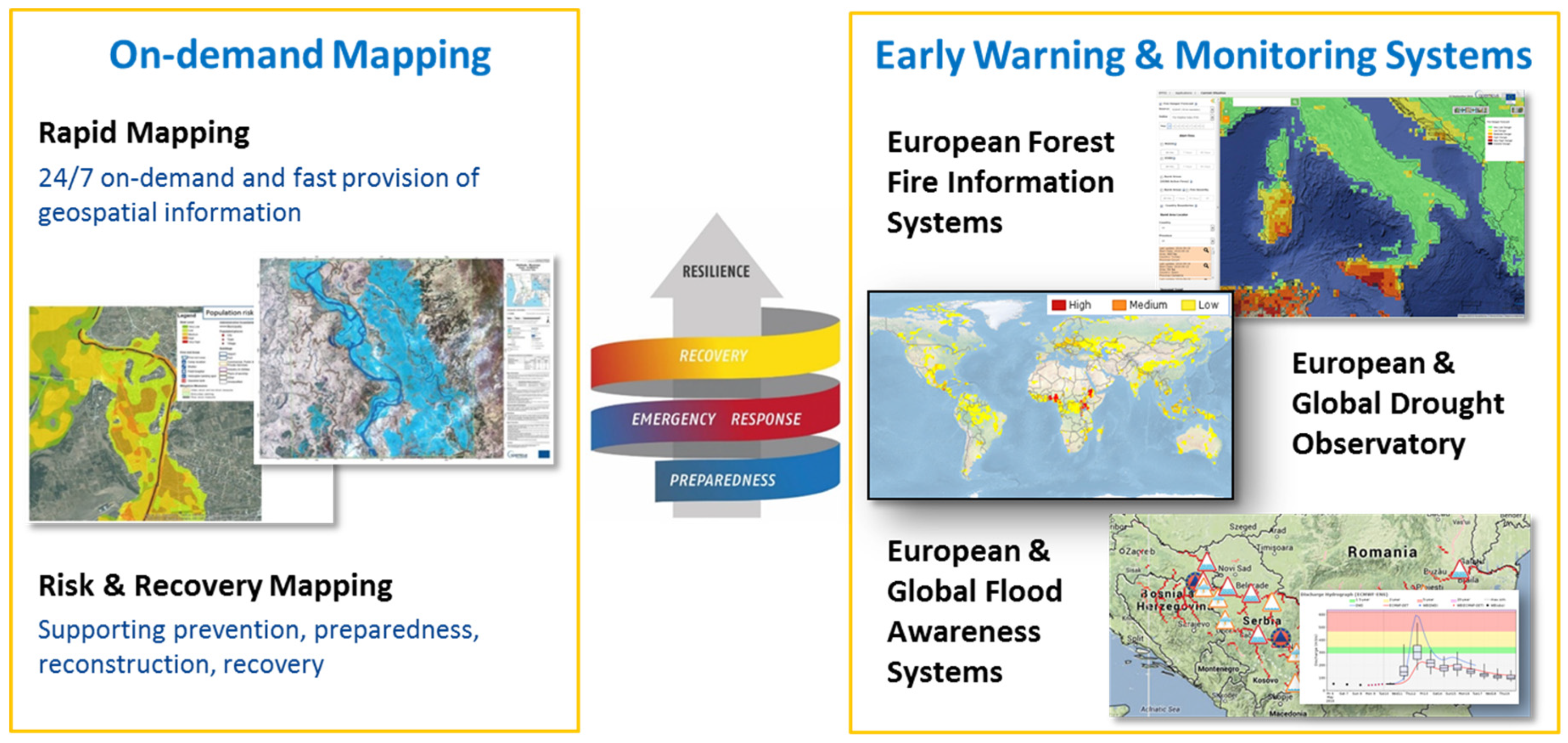
The Copernicus Emergency Management Service (CEMS) is one of the six services offered by Copernicus, the European Union’s Earth Observation programme for global environmental monitoring, disaster management and security. CEMS provides support to all actors involved in the fields of crisis management, humanitarian aid as well as disaster risk reduction, preparedness and prevention. The service has two main components: Early Warning and Monitoring, and On-demand Mapping services. The Early Warning and Monitoring component provides continuous and global information about floods, forest fires and droughts. Instead, the services of the On-demand Mapping component are providing geographic information on-demand for a specific disaster (any type of natural or man-made disasters, globally) and a limited area. Figure 1 depicts the general service overview. The On-demand Mapping component includes a SEM mechanism which will be described hereafter.

CEMS On-demand Mapping is managed by the Joint Research Centre (JRC) and operated through the Emergency Response and Coordination Centre (ERCC) at the European Commission’s Directorate-General for Humanitarian Aid and Civil Protection (DG ECHO). It has been operational since April 2012 and provides geospatial information, maps and analyses based on satellite imagery acquired before, during or after a disaster. It can be triggered only by Authorised Users which include National Focal Points in the European Union Member States and in most countries participating in the European Civil Protection Mechanism, as well as European Commission services and the European External Action Service. Other local and regional entities, International Governmental Organisations (e.g., UN agencies, World Bank), and National and International Non-Governmental Organisations can activate the service through an Authorised User.

Depending on the need of the user and for which phase of the disaster management cycle geo-information is required, it is provided in two different modes: Rapid Mapping or Risk and Recovery. They differ in terms of map delivery times, type of analysis performed and level of standardization in the workflow. Rapid Mapping provides geo-information within hours or days, immediately following the event (fast provision). With its 24/7 availability, it supports emergency management activities immediately following an emergency event and is thus the SEM mechanism of CEMS. Both, workflow and products are standardized to allow fast handling of requests and meeting target delivery times. On the other hand, Risk and Recovery operates during working days and working hours only. It is designed for pre- or post-crisis situations which do not require immediate action and provides geo-information within weeks or months after the service activation in support of recovery, disaster risk reductions, prevention, and preparedness activities. The geo-information and other results generated by both mapping modes are accessible on the CEMS mapping portal (emergency.copernicus.eu/mapping). Like all Copernicus core services, the products are free of charge.

The specific service tasks, including image ordering and analysis, are carried out by service providers (i.e., operating entities) who are consortia of European companies, academia and public institutions.

2.2.1. Rapid Mapping

Copernicus EMS Rapid Mapping (CEMS-RM) covers the entire process from the satellite tasking, image acquisition, processing and analysis of satellite imagery and other geo-spatial raster and vector data sources until the production and delivery of vector data and ready-to-print maps to the user who requested the service. Since its start in April 2012, it has been activated 352 times, and 6% of these activations were for earthquakes (as of 10 April 2019).

CEMS-RM products are standardized maps with a set of parameters to choose from when requesting the service activation (map type, scale, delivery time, additional information layers to be included).

Table 1. Rapid Mapping portfolio: product types and production times (two service levels). Note that for delineation and grading a First Available Map (an early information product) is available within 3 h from image reception in the 24/7 service level.

Product Type	Content	Delivery Times after Image Reception in the Two Service Levels
		24/7 (hours)	Production during working days (days)
Reference	Pre-event situation	9	5
Delineation	Detailed assessment of the impacted area (extent)	12	5
Grading	Detailed damage assessment (damage grade and its spatial extent)	12	5

shows the product portfolio. There are three map types, one pre- and two post-event maps, each performing specific functions relevant to crisis management.

The pre-event or reference maps provide comprehensive knowledge of the territory and exposed assets and population. They are based on satellite imagery and other geo-spatial data acquired prior to the disaster event and are often used for comparative purposes as a baseline for generating the post-event maps. The two post-event map types, known as delineation and grading map, are produced from post-disaster images. Delineation maps outline the extent of the area affected by an event and its evolution. Grading maps provide an assessment of the impact caused by the disaster in terms of damage grade and of its spatial distribution. They may also provide relevant and up-to-date information on affected population and assets, e.g., settlements, transport networks, industry and utilities. Grading maps are therefore the most relevant product for events like earthquakes and tsunamis: through the location of affected assets, they reveal indirectly the spatial extent of the impacted area.

As detailed in Table 1, the service provides both post-event maps within 12 h after image data reception and quality acceptance in the fastest map production mode. For less time-critical activations, the same maps can be provided in five working days. Reference maps are provided either in nine hours (fastest mode) or in five working days.

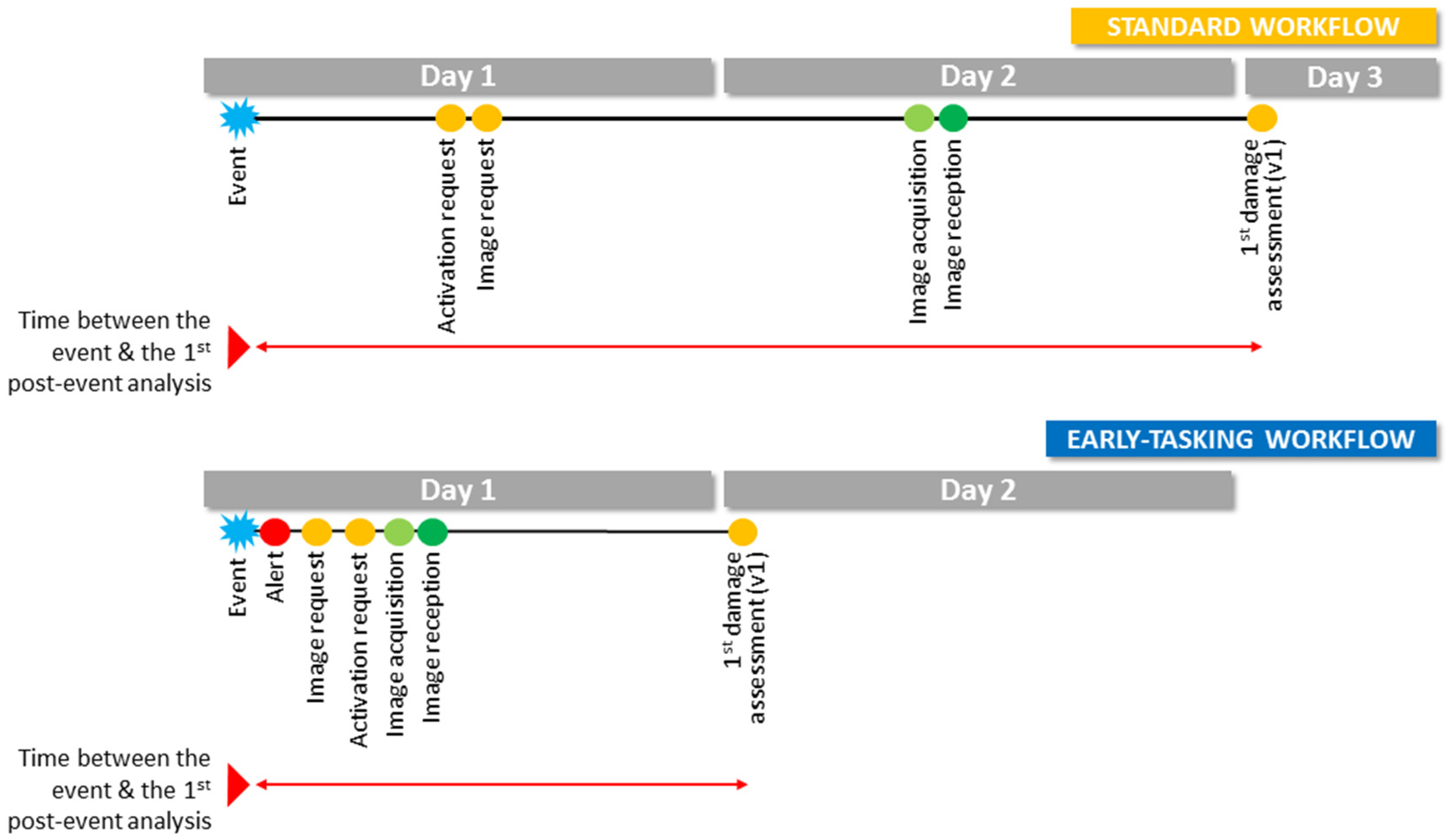
Satellite images being the main source of information for CEMS-RM, it is evident that satellite tasking is a key phase for the effectiveness of the service. CEMS-RM is currently testing a procedure which implies using early warning information on upcoming floods to trigger an image-tasking request 24 h before the expected flood peak. Following the same logic, alert systems like GDACS can be used to trigger satellite tasking (or encourage satellite mission owners to task their satellites) over a possibly affected area shortly after the alert and before an actual activation of CEMS-RM following the required request by an authorised user. This would allow having relevant imagery once the activation is triggered. Despite technical limitations of tasking satellites for a new acquisition (orbits, cut-off-times for scheduling a new tasking), experience over the past six years has shown that time can be gained by submitting a tasking as soon as there is a very high probability that an event will occur (e.g., floods, tropical storms) or as soon as an event has occurred (e.g., earthquakes, tsunamis, volcanic eruptions). Statistics (from 2012 to 2019) for CEMS-RM activations for earthquakes which started within 24 h after the event show that the time lapse between the earthquake and the reception of an activation request is 12 h on average (in a range from 0.5 to 21 h considering 16 activations). This time could lead to a delay of up to one day as the request often comes too late for an acquisition on the same day (due to the aforementioned tasking limitations). Figure 2 shows the potential benefit of a satellite early tasking based on early warning information compared to the standard workflow. The example shows the timeline for a hypothetic event which occurs in the first hours of the day. In this example up to one day can be gained when early warning information is used.

3. Results: GDACS Tsunami Model and CEMS Rapid Mapping Activation Outputs for the 2015 Tsunami in Chile

In the aftermath of the tsunami generated by the earthquake on 16 September 2015 in Chile, 30,000 e-mails and 18,000 SMS messages were dispatched by the GDACS few minutes after the event, providing information on the potential impact along the Chilean coast.

The European Union’s Emergency Response Coordination Centre in Brussels (DG ECHO-ERCC) activated the Rapid Mapping component of CEMS about nine hours after the event.

3.1. GDACS Tsunami Model Outputs

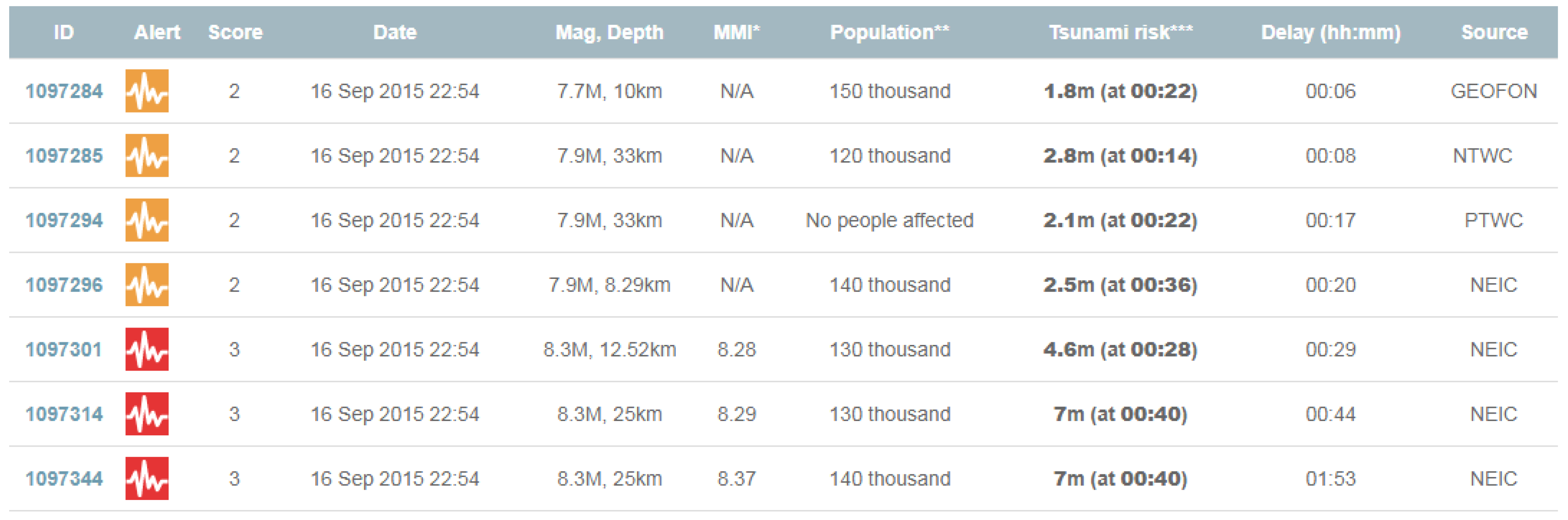
The event timeline shown in Figure 3 highlights that several re-runs of the tsunami model were carried out (with a delay in the range of a few minutes to ~2 h), depending on the availability of more precise earthquake parameters. For this reason, the type of alert ranges from orange to red and the tsunami impact (in terms of max height) increases from 1.8 m to 7 m.

Although GDACS is an automatic system and all the estimations are based on event detection and launch of dedicated calculations, the last value of the impact estimation (which is used as reference in this contribution) has been obtained by performinga manual calculation ~2 h after the event, when more precise information on the fault mechanism were available from USGS (http://earthquake.usgs.gov/earthquakes/eventpage/us20003k7a), as detailed in

Table 2. Epicenter.

Parameter	Value
Latitude (WGS84)	31.60° S
Longitude (WGS84)	71.70° W
Magnitude	8.3 mww
Depth	22.4 km, middle of fault, hypocenter
Water Depth	−232 m
Event Date	16 September 2015 22:54:32 (UTC)

and

Table 3. Fault geometry.

Parameter	Value
Displacement	6	(m)
Width	62	(km)
Length	223	(km)
Strike	353	(deg.—North = 0 deg.)
Dip	19	(deg.)
Rake	83	(deg.)

.

Table 4. First 20 locations reached by the tsunami wave (the whole list of locations can be accessed as a KML file in the GDACS report: http://webcritech.jrc.ec.europa.eu/ModellingTsunami/TsunamiSurge/JETS_System/2015/09/17370/locations.kml).

Arrival Time (UTC)	Date/Time of Max Height (UTC)	Location	Height (m)	Lat/Lon (WGS84)
16 September 2015 22:56	16 September 2015 23:34	Chigualoco	7.0	31.75° S	71.50° W
16 September 2015 22:56	16 September 2015 23:10	Conchali	4.6	31.88° S	71.49° W
16 September 2015 22:56	16 September 2015 23:08	Los Vilos	4.4	31.92° S	71.51° W
16 September 2015 22:56	16 September 2015 23:06	Huentelauquen	4.0	31.58° S	71.53° W
16 September 2015 22:56	16 September 2015 23:10	El Romeral	3.9	32.42° S	71.38° W
16 September 2015 22:56	16 September 2015 23:02	Angostura	3.1	31.50° S	71.55° W
16 September 2015 22:56	16 September 2015 23:04	Totoralillo	3.1	32.04° S	71.52° W
16 September 2015 22:56	16 September 2015 23:04	Quilimari	2.9	32.12° S	71.49° W
16 September 2015 22:56	16 September 2015 23:04	Pichidangui	2.9	32.13° S	71.53° W
16 September 2015 22:56	16 September 2015 23:06	Ingeniero Santa Maria	2.6	32.23° S	71.47° W
16 September 2015 22:56	16 September 2015 23:00	Quillaicillo	2.6	31.41° S	71.57° W
16 September 2015 22:56	16 September 2015 23:06	Guaquen	2.6	32.30° S	71.45° W
16 September 2015 22:56	16 September 2015 23:00	Maitencillo	2.5	30.99° S	71.64° W
16 September 2015 23:02	16 September 2015 23:14	Concon	2.2	32.94° S	71.52° W
16 September 2015 23:02	16 September 2015 23:14	Las Ramaditas	2.2	32.92° S	71.50° W
16 September 2015 22:56	16 September 2015 23:08	Papudo	2.2	32.51° S	71.45° W
16 September 2015 22:56	16 September 2015 23:08	Pite	2.2	32.52° S	71.48° W
16 September 2015 22:56	16 September 2015 23:04	Gauchal	2.0	31.77° S	71.47° W
16 September 2015 23:20	17 September 2015 01:04	La Boca	2.0	33.92° S	71.84° W
16 September 2015 22:58	16 September 2015 23:54	Ritoque	1.9	32.82° S	71.52° W

reports the list of the first 20 locations reached by the Tsunami wave according to the outputs of the tsunami model run. The full list of location is available at the GDACS website (see http://www.gdacs.org/report.aspx?eventtype=EQ&eventid=1065792).

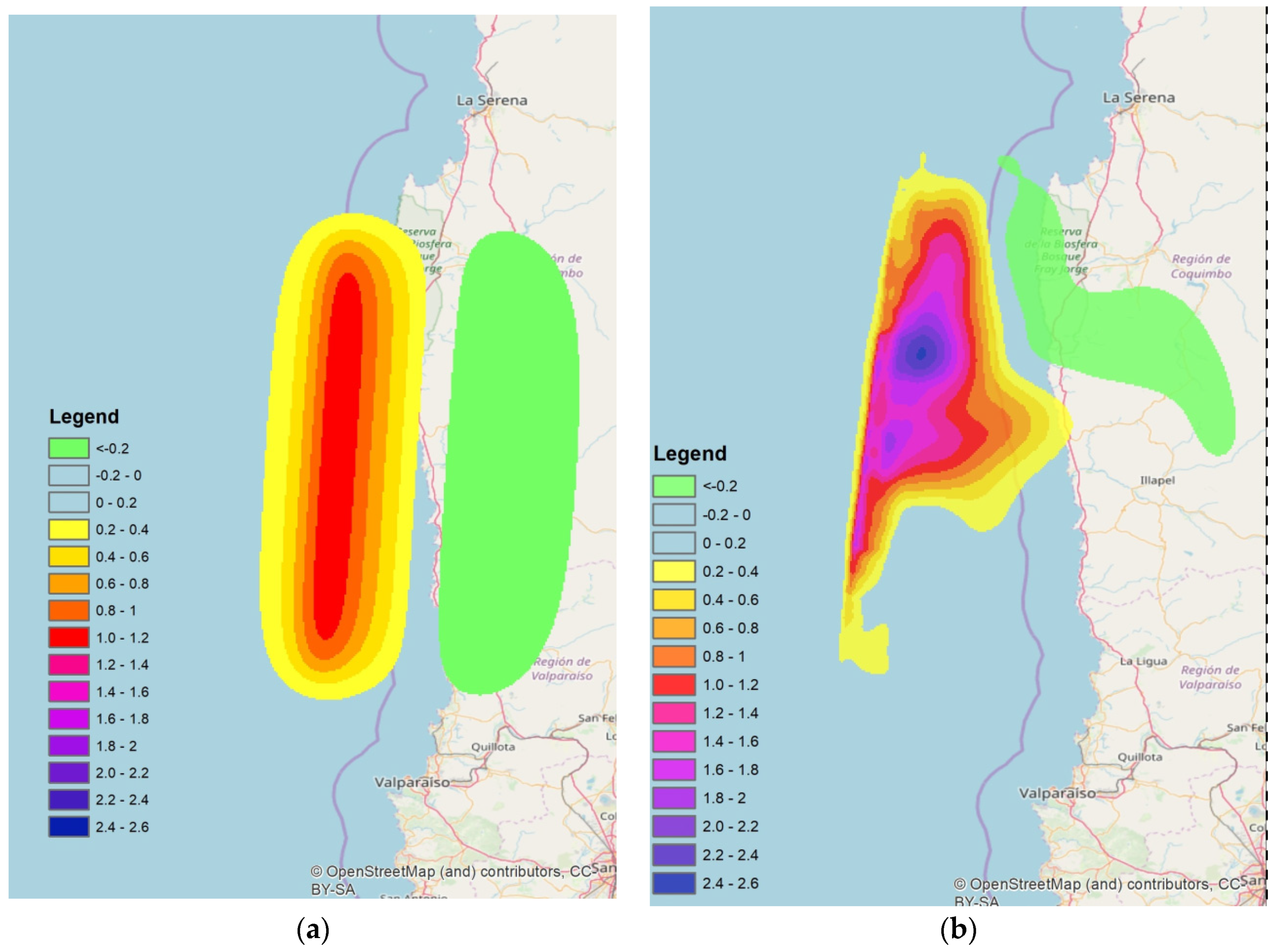
The estimated maximum height is 7.0 m in Chigualoco (31.75° S, 71.50° W) but many other locations were estimated to have been severely impacted by the tsunami wave, as shown in Figure 4.

In the analysis the GEBCO 30 s bathymetry has been used: in the coarse calculation (Figure 4a) the original GEBCO bathymetry was resampled at 1.75 min (3.5 km) while in the more refined calculation (Figure 4b) a down sampling to 0.25 min was adopted.

Validation of the GDACS Tsunami Model: Tidal Gauge and Post-Event Field Survey

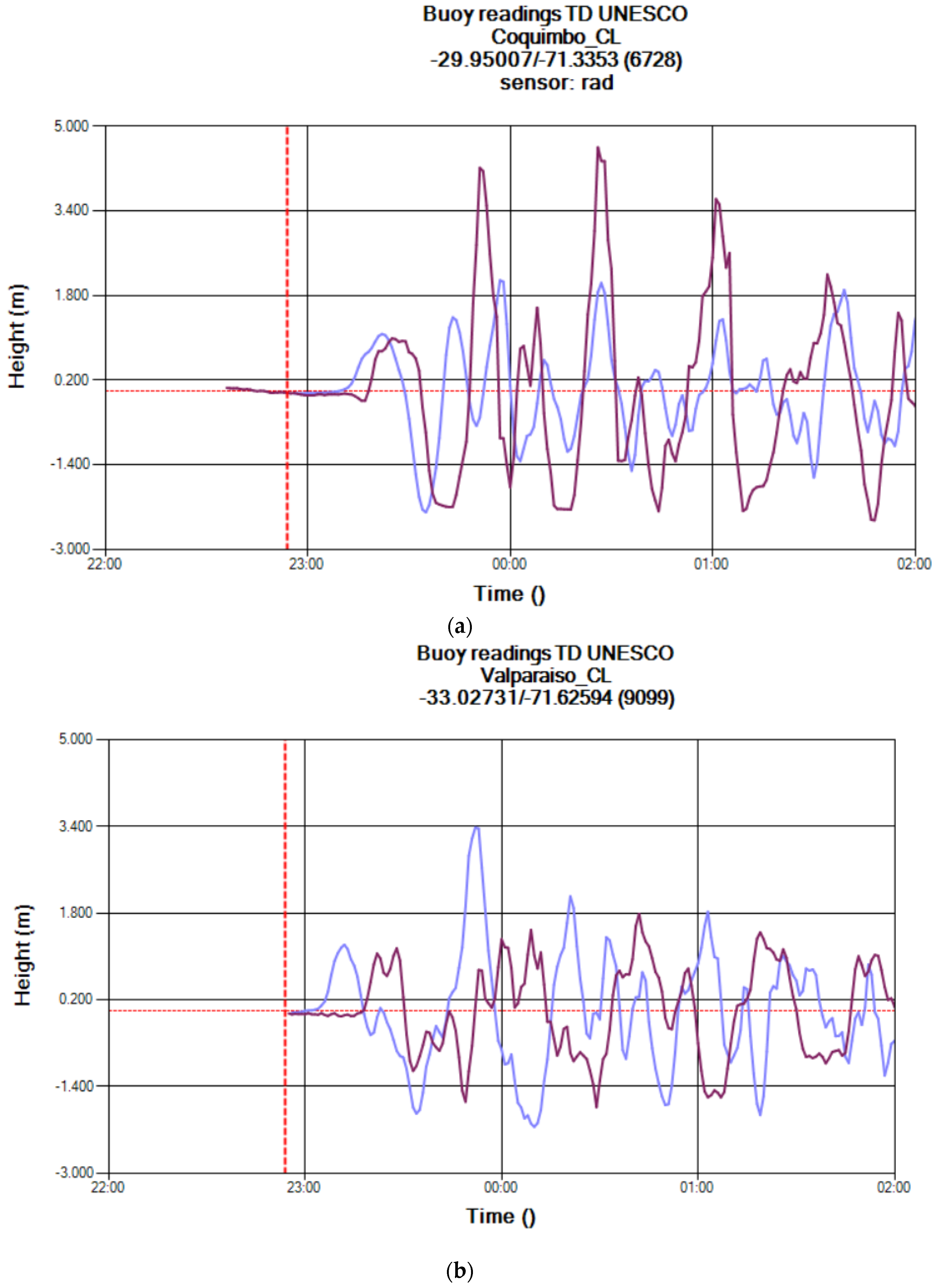
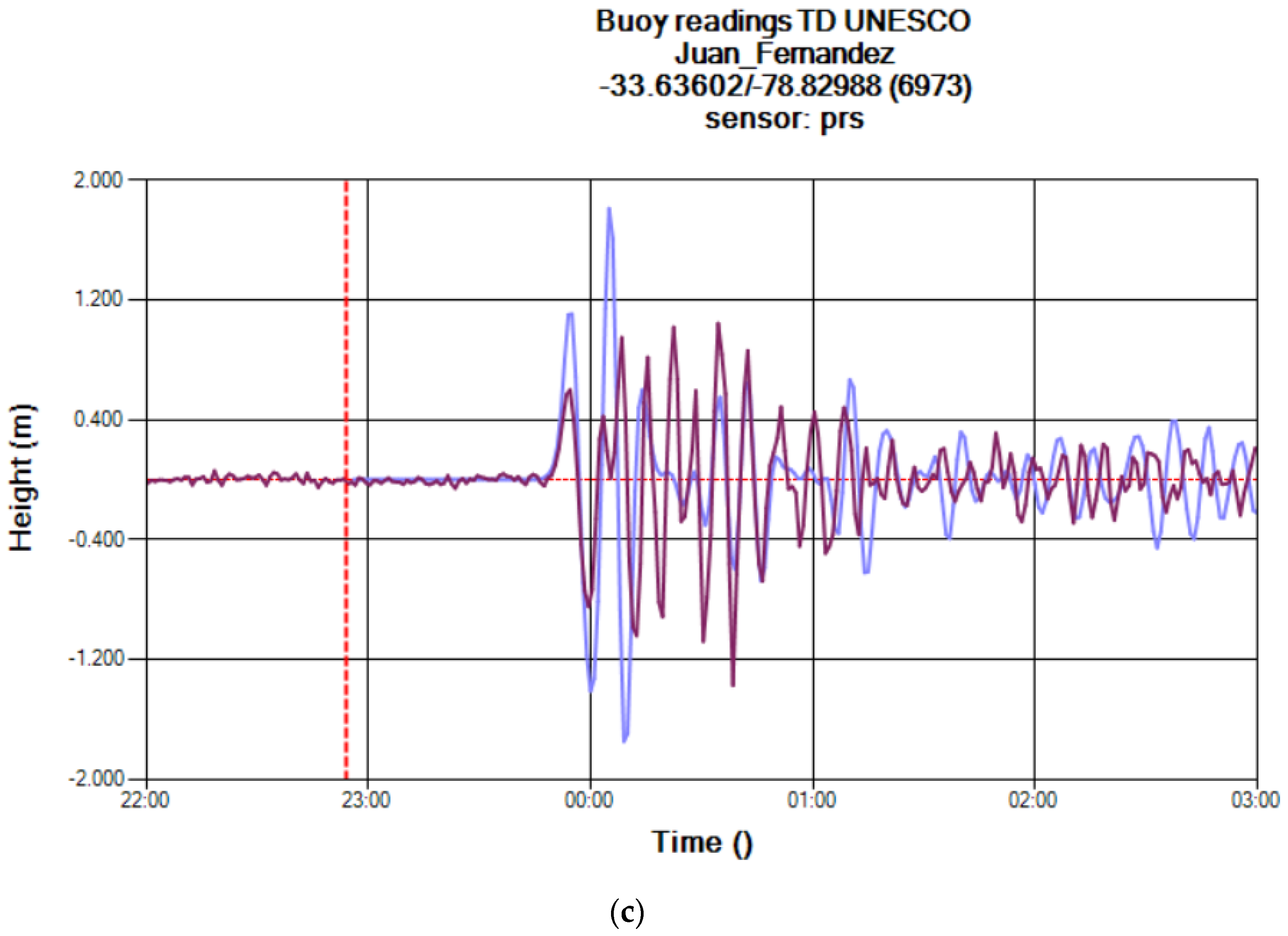
The comparison between measured and calculated sea levels allows the quality of the calculation to be assessed. To this end, expected wave height and sea level measured by tidal gauges are compared in three different locations: Coquimbo, Valparaiso and the Juan Fernandez Island (respectively green triangles 1, 2 and 3 in Figure 4). The comparison of the predicted and measured graphs shows that, although the absolute height of the measured and estimated values seem to mismatch, the main features of the event are captured by the calculations (i.e., level rising at the right moment, similar periodic oscillations), as shown in Figure 5. In particular, it can be noted that the sea level shows several periodic peaks induced by the bathymetry in front of the Chilean coast that causes wave reflection (sloshing) with increasing wave heights. In Juan Fernandez the arrival time and the period are predicted correctly while the amplitude is slightly overestimated. The quality of the calculations cannot be improved considerably in this type of on-the-fly calculations with a uniform source, as shown in the next paragraphs focused on the comparison with the survey data.

A comprehensive validation of the model outputs was carried out exploiting also a very detailed survey conducted along the coast by a post-tsunami survey team composed of local researchers and deployed from 17 September to 14 November 2015 [4]. The survey covered approximately 80 sites (both coastal towns with evident damage and isolated sites where the tsunami signature remained almost intact) along 500 km of the primary impact zone, from the northernmost site where damage was reported, Bahía Carrizalillo (29.11° S, 71.46° W), southward to El Yali National Reserve (33.75° S, 71.73° W) beyond which no tsunami damage was reported.

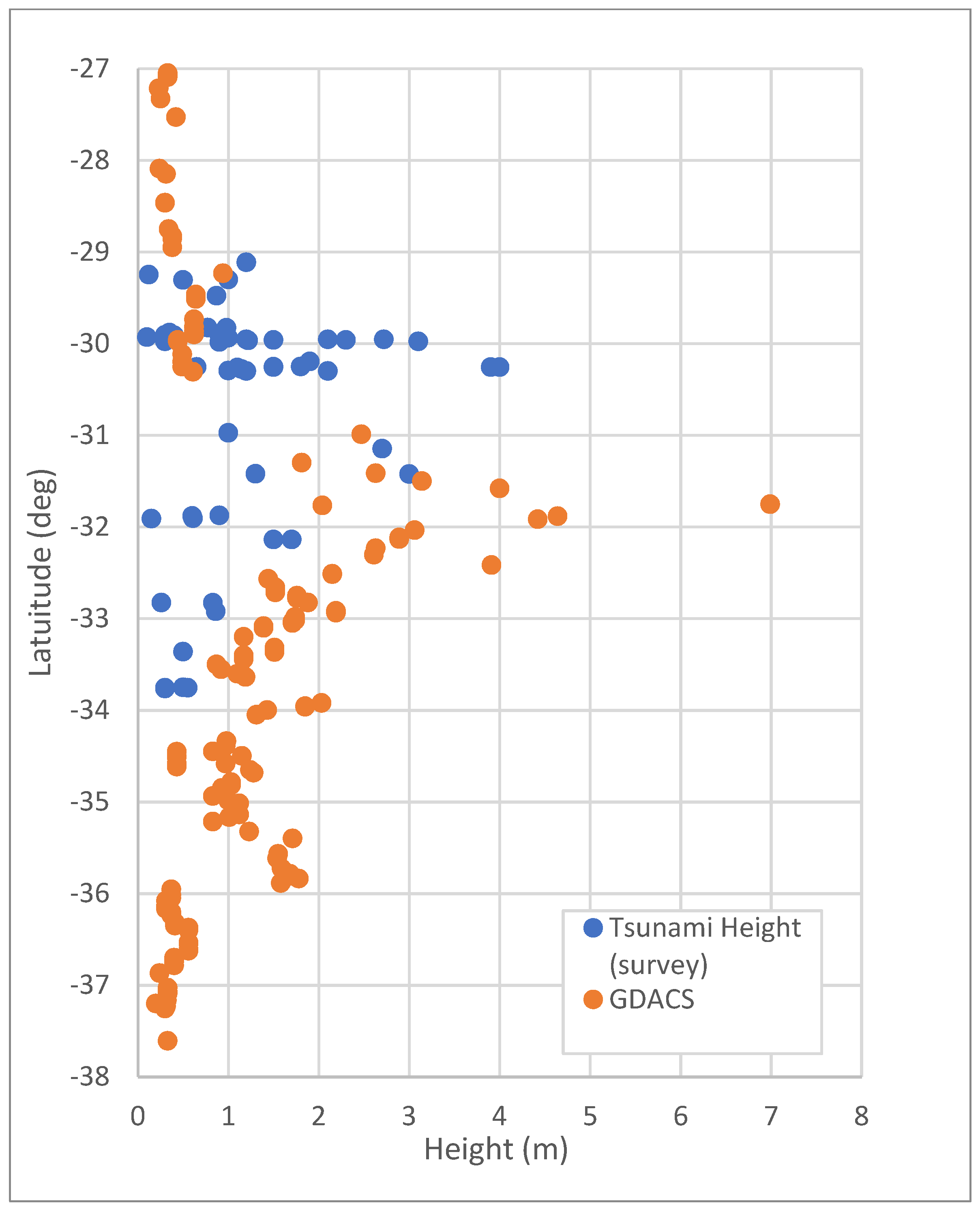
The detailed analysis shows that the initial estimates of the major damage in the coastal range were correct, even if the computed range with heights exceeding 1 m (latitude in the range from 35.88° S to 30.98° S) were expected further south than where they actually occurred (latitude in the range from 33.76° S to 29.82° S). Figure 6 shows a comparison of the measured and the estimated tsunami height.

The reason for the southern shift of the maximum impact is mainly due to the actual type of fault. In the minutes after the event a detailed fault mechanism is unknown and therefore a uniform deformation plane centered on the epicenter is assumed (Figure 7a). In reality the epicenter is only the starting point of the deformation which is not uniformly distributed along the fault plane. The finite fault model (Figure 7b) from the United States Geological Survey (USGS, https://earthquake.usgs.gov/earthquakes/eventpage/us20003k7a/finite-fault) shows that the deformation started from the epicenter but most of it occurred northern off-centered. In general, the finite fault model is able to explain better the results of an event but unfortunately this solution is not available at the time of the event but only hours or days after the events. Additionally, the adoption of the output of a Finite Fault model requires detailed editing that cannot be performed automatically.

One possible method to try to overcome the difficulties in the forecast of the initial source is the performance of several calculations by modifying the initial conditions with a certain range of possible values. A Monte Carlo type of analysis is under development to include in the possible calculations results the parameters uncertainty. It will always quite difficult to try to estimate the finite fault model as it is very complicated and impossible to forecast but at least a range of possible solutions can be identified.

3.2. CEMS Rapid Mapping Activation Outputs

Details and products of the activation for this event are available on the public website under activation code [EMSR137]: Earthquake in Chile (https://emergency.copernicus.eu/mapping/list-of-components/EMSR137). In their first request the ERCC requested mapping the area of Coquimbo city and surroundings (Detail 01 in Figure 8). The definition of these areas was based on knowledge from the ground and media reports. Soon after, several areas were added over populated places along the coast ~300 km south of Coquimbo based on an analysis of the tsunami impact estimate released by GDACS (Detail 02 in Figure 8).

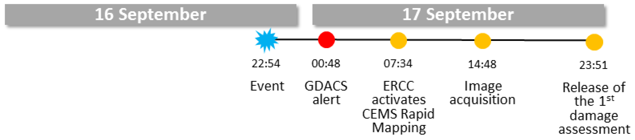
The first results of the satellite-based impact assessment were published 25 h after the earthquake (a series of six maps covering the area of Coquimbo). For the assessment, very high resolution optical imagery (sub-meter resolution), acquired ~16 h after the event, was used. Figure 9 shows the main steps from the earthquake to the GDACS alert, the activation of CEMS-RM by the ERCC, the acquisition of the image to the release of the first results of the damage assessment. The timeline for this CEMS-RM activation was extremely good considering that the service provided first information within 16 h after the user request (service target is 24 h). Crucial was the scheduling of the new satellite tasking over the affected areas at such short notice (confirmation of the afternoon tasking during the morning of the same day). As detailed is Section 2.2.1, this generally takes one day, depending on when the request is submitted with respect to the satellite tasking cut-off times. In this specific case by the time the tasking request was submitted, the image provider had already proactively planned a tasking over the area and CEMS-RM could benefit from it.

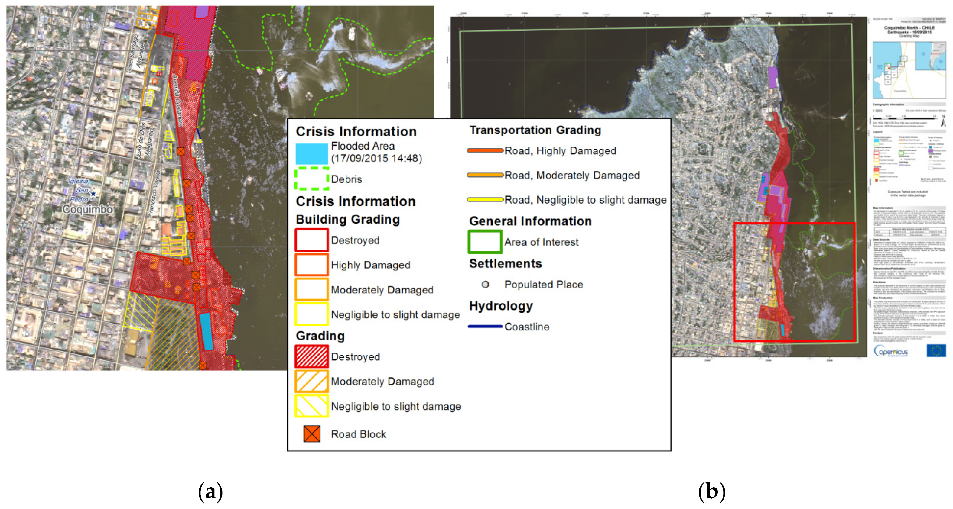
Figure 10 below shows an example of the released map products. The result of the assessment highlights affected assets (buildings, facilities, roads) in an area of 100–200 m inland and along the coast of Coquimbo city (first set of areas, Detail 01 in Figure 8). The assessment of the areas which were defined based on GDACS’ impact assessment (Detail 02 in Figure 8) revealed only minor damage.

3.3. Early Tasking Approaches Based on the Tsunami Model Output

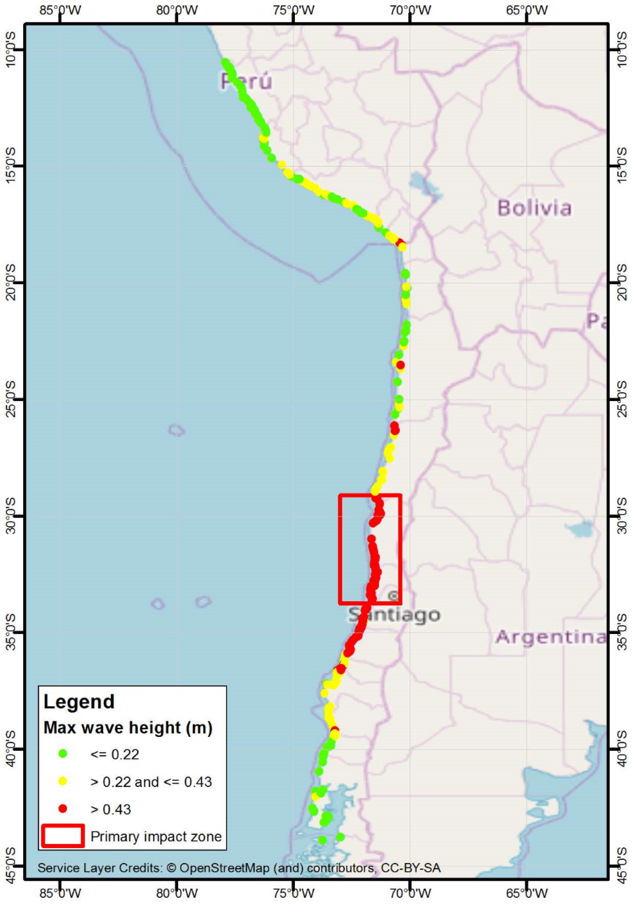
According to [4], the tsunami primary impact zone is distributed along approximately 5000 km of the Chilean coast. The locations resulted as affected by the tsunami model are distributed along more than 4000 km of the Peruvian and Chilean coast, from 10.57° S to 43.90° S. Considering only the 3rd quantile of the distribution of the estimated wave height on the coast (>0.43 m), the length of the coast possibly impacted is approximately 2300 km, from 18.30° S to 39.21° S (Figure 11).

Assessing the damages caused by the tsunami over the whole length of the Pacific coast possibly affected by the tsunami on the basis of the model outputs is not feasible for a SEM mechanism, mainly for the following reasons:

• tsunami damage assessment based on satellite data requires very high resolution (VHR) optical imagery. Even assuming that one or more satellite data providers can cover similar extents with the required resolution exploiting (virtual) constellations, the related data costs would be extremely high;
• even if CEMS-RM benefits from the possibility to plan acquisitions for most of the satellite data providers (Copernicus contributing missions), the current mechanism activations on large areas increase the possibility to generate tasking conflicts (possibly also with other SEM mechanisms) which may result in losing time and in the worst case even missing an acquisition opportunity;
• the possibly impacted area is significantly larger than the maximum capacity of the service, leading to significant delays in the generation of products;
• CEMS-RM production costs (for damage assessments currently visual interpretation is the standard approach) are proportional to the area examined and an extent similar to the one in discussion would not be sustainable.

Therefore, it is crucial to prioritize the areas where to trigger satellite acquisitions and perform satellite-based damage assessment. The optimum would be to have an automatic prioritization process to identify the areas of interest in the shortest time frame possible to avoid delay in the post-event image acquisition (as discussed in Section 2.2.1).

In order to automatically prioritize the areas for satellite acquisitions, three different approaches based on integration of tsunami model outputs and exposure data are proposed, described and discussed, namely:

• Maximum wave height and populated place categories
• Maximum wave height and population estimates
• Maximum wave height and number of buildings

The aforementioned approaches are all based on geoprocessing workflows generating 3-class impact indexes in form of 0.25° by 0.25° raster outputs providing information on relative priorities among the impacted areas. Given the lack of additional case studies to further validate the proposed approaches, the current analysis is limited to a detailed discussion on benefits and drawbacks of each method. Further tests will be carried out on future major tsunami events for which also a SEM response will be in place.

3.3.1. Maximum Wave Height and Populated Place Categories

The tsunami model estimates the maximum wave height impacting on a set of locations distributed along the coast. By simply dividing the estimated maximum wave height with the city class (which can be considered a proxy of the population) in the range from 1 to 6 (the classes used by Europa Technologies Global Insight Plus dataset, where value 1 indicates that the place is a capital, 2 is a major city running down to 6 which indicates a village or other minor settlement: https://www.europa.uk.com/map-data/global-map-data/global-insight/global-insight-faq/) it is possible to obtain an index that takes into consideration the exposure (expressed as importance of the location) where higher values represent locations more at risk. 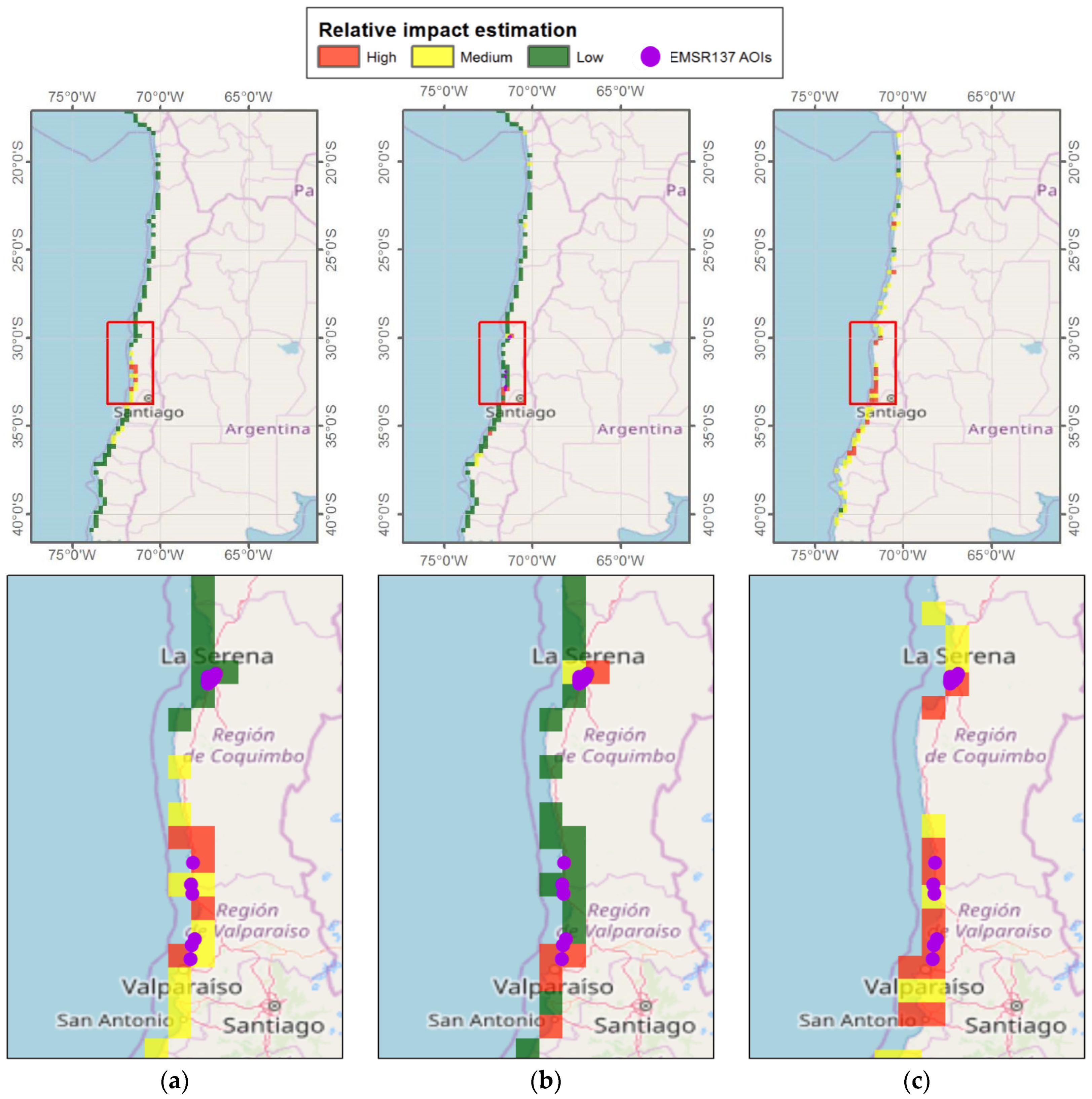Classifying such index in 3 classes based on the Jenks natural breaks classification method [5] and then grouping together adjacent pixels in the same class, 3 areas of interest with higher priority and other 5 with lower priority (Figure 12a) are identified. With the proposed approach, one of the most affected areas, La Serena and Coquimbo, were not identified, due to both the latitudinal shift of the estimated maximum wave height compared to the measured one (as shown in Figure 6, leading to values lower than 1 m in such areas) and the relatively low importance in terms of inhabited location class (both are in city class 3).

The main drawback of a similar approach is related to the heterogeneous accuracy, incompleteness and level of update of the populated places categories.

3.3.2. Maximum Wave Height and Population Estimates

This approach exploits a population estimate dataset as exposure information. Specifically, the following empirical formula is proposed:

Relative impact index = Log (k Pop) H_max

(1)

where:

• Pop is the population in an arbitrary radius of 6 km from the affected location coordinates.
• k is a factor that changes the relative weight of the population versus the tsunami impact.
• Hmax is the maximum wave height estimated in the affected location.

In the proposed scenario, k has been set equal to 0.0001 to avoid overweighting the population with respect to the wave height. Such value is a first attempt to identify the best balance between tsunami wave height and population exposure; a more systematic analysis based on future events is necessary to confirm that this value can be properly generalized. As a population data source, the Landscan (https://landscan.ornl.gov, 2016 edition) dataset has been used. According to this approach, 3 high priority and 1 medium priority areas for satellite tasking are identified (Figure 12b). It can be noted that only one area was identified as high priority in both methods covered so far, clearly highlighting the crucial role of the type of exposure data exploited in the estimation of the relative impact.

3.3.3. Maximum Wave Height and Number of Buildings

To be independent from population datasets or populated places categories and to exploit a potentially more updated dataset, the authors explored the possibility to use a different proxy for identifying the level of exposure of each location, i.e., the number of buildings in the areas identified as being at risk by the tsunami model output. In this specific case, OpenStreetMap (OSM), a map of the world created by volunteers and free to be used under an open license, has been adopted as a source for building dataset. Among the features present in OSM, building footprints are among those considered more relevant, especially for emergency response: for this reason, building footprints together with the road network, are the most requested features to be digitized by Humanitarian OpenStreetmap Team (HOT) volunteers, the humanitarian branch of OSM mobilized after major emergencies.

In the specific case study, as of 12 April 2019 almost 120,000 OSM building footprints are present in the areas identified as affected by the tsunami model. Those building footprints have been associated with one of the tsunami affected locality based on a proximity criterion: every building footprint within 5 km from an affected locality has uniquely been assigned to its nearest locality. In this way, it has been possible to enrich the locality attributes by adding the number of buildings associated to each of the locations.

By simply combining 3 classes (based on quantile classification method) of estimated maximum wave height and number of buildings in each potentially affected location, it is possible to identify four clusters that can be used to define higher priority areas of interest (AOIs): La Serena/Coquimbo, 2 areas North of Valparaiso and San Antonio (Figure 12c). The first 3 clusters correspond to the actual AOIs of the CEMS-RM activation.

The main advantage of this approach, in comparison with the previous two, is to provide an overall better correspondence between the priority level and the actual damages: i.e., the EMSR137 AOIs are all located in correspondence with red or yellow pixels. Furthermore, a shorter portion of the coast between La Serena and Valparaiso, where no actual damage has been reported, is estimated as possibly impacted. The main disadvantage of this approach is that most of the overall impact area is flagged as medium and high priority, partially failing in addressing the goal of having a relative estimation of the impact level for immediate decision making. Additionally, the main concern in adopting a similar approach is related to actual availability and coverage of building information in the immediate aftermath of a specific event: despite the high number of registered users (including the HOT-OSM community) and although nodes and ways are constantly growing in OSM and the amount of OSM information increases over specific areas where a disaster occurs, there is a risk that the same area may be not covered at all by OSM when the priority areas must be identified. Other datasets of human presence at coarser resolution and global scale can, therefore, be used for the impact estimate, as detailed in Section 4.

4. Discussion and Conclusions

The main goal of the research was to identify and evaluate possible operational solutions to further improve the timeliness of SEM services such as the CEMS-RM. To this purpose, one of the key aspects is to establish a closer link between early warning and alert systems, such as GDACS, and CEMS-RM.

Section 3.1 demonstrated the benefit of integrating early warning and alert systems in SEM. Even if the first tsunami impact estimate for the Chilean earthquake did not succeed in identifying the areas which suffered the biggest impact in terms of damages (mainly due to the unavailability of the precise finite fault model in the first hours after the event, which led to a latitudinal shift in the estimated maximum weight heights), the possibly affected areas were among those identified.

Having access to information on possibly affected areas is crucial for obtaining useful information from SEM. With ongoing research on tsunami modeling (and the availability of faster source mechanisms identification at global level), and through validation of actual events, the accuracy of impact estimates is expected to improve in the near future.

Additionally, a Monte Carlo calculation strategy has already been planned to provide not only the expected tsunami wave height but also its uncertainty range, by varying the initial and boundary condition of the simulations. Despite the discussed limitations, the overall goal would be to correctly identify some of the major affected areas, considering that the impact of true positive is operationally of greater importance than possible false positives (leading to acquisition of satellite imagery over non-affected areas).

To exploit such alerts in a SEM workflow operationally, the outputs need to be properly integrated with exposure information, as described in Section 3.3.

The three proposed approaches are all based on different proxies or estimates of the population living in the impacted areas: the differences in the identified priority areas are due to the different level of accuracy, completeness and update of such datasets. Therefore, the availability of homogeneous and global data sources, focusing not only on population but also on built-up areas, is crucial. Initiatives like the EC-JRC Global Human Settlement (GHS) framework address this need, producing global spatial information about the human presence on the planet over time [6] in the form of built up maps, population density maps and settlement maps. This information is generated with evidence-based analytics and knowledge using new spatial data-mining technologies and is ready to be integrated in the workflow (work in this respect is ongoing).

The analysis of the proposed approaches also highlights that the focus should be on integrating different types of exposure information (e.g., a mix of the approaches described in Section 3.3.2 and Section 3.3.3), especially considering that a clear understanding of the dynamics of the built environment and how it affects, in case of natural disasters, the life of communities, may lead to a substantial reduction of disaster risk and loss of life [7,8,9,10]. For instance, initiatives like the OpenBuildingMap system (http://obm.gfz-potsdam.de/) systematically harvest building footprints from OSM and derives exposure and vulnerability indicators from explicitly provided data (e.g., hospital locations), implicitly provided data (e.g., building shapes and positions), and semantically derived data, i.e., interpretation applying expert knowledge [11].

Unfortunately, the lack of major events for which SEM response was in place and the underlying datasets were available, did not allow the authors to further test the proposed approaches. Additional tests are planned for future major events, with the goal to further evaluate the proposed approaches and to potentially fine tune the underlying methods, identifying a unique operational workflow.

CEMS-RM is continuously seeking to improve timeliness of the service and uses as much as possible information which is available in the first hours after events. In this view and to further exploit this information, an additional product was recently introduced in CEMS-RM (since April 2019). The First Estimate Product (FEP) is an early information product which aims at providing an extremely fast (yet rough) assessment of most affected locations within the area of interest. FEP can be used to (1) highlight possibly affected areas, (2) review the initial product specifications (product type, areas of interest) or (3) decide on cancellation of initially requested delineation or grading products. In the current setup, FEP information is derived from the earliest suitable available post-event image. Rapid tsunami loss estimation can represent an effective way to generate a FEP [12]: coastal area inundation parameters (extent and maximum water height) derived from models and integrated with available exposure data, provide information that can be exploited to quickly generate first damage estimates, without waiting for the availability of any post-event image. In big disasters like tsunamis, FEP helps researchers to understand the situation quickly and supports the identification of focus areas for further image tasking and analysis.

Lastly, it has to be remarked that in the last few years new satellite constellations composed of hundreds of small platforms provide daily high-resolution images of the entire Earth, i.e., the 3 m Planet data. A similar capacity shifts the focus from identifying the priority target areas for satellite sensing to how to efficiently extract useful information from a huge amount of data. This is the main reason why the trending research topics in the SEM domain deal with how to quickly generalize pre-trained deep learning networks to identify areas affected by disasters. While waiting for algorithms with sufficiently high accuracy and complete level of automation, there is still the need to identify the high priority areas to be interpreted by image analysts.