NN-Based Prediction of Sentinel-1 SAR Image Filtering Efficiency

Abstract

Images acquired by synthetic aperture radars are degraded by speckle that prevents efficient extraction of useful information from radar remote sensing data. Filtering or despeckling is a tool often used to improve image quality. However, depending upon image and noise properties, the quality of improvement can vary. Besides, a quality can be characterized by different criteria or metrics, where visual quality metrics can be of value. For the case study of discrete cosine transform (DCT)based filtering, we show that improvement of radar image quality due to denoising can be predicted in a simple and fast way, especially if one deals with particular type of radar data such as images acquired by Sentinel-1. Our approach is based on application of a trained neural network that, in general, might have a different number of inputs (features). We propose a set of features describing image and noise statistics from different viewpoints. From this set, that contains 28 features, we analyze different subsets and show that a subset of the 13 most important and informative features leads to a very accurate prediction. Test image generation and network training peculiarities are discussed. The trained neural network is then tested using different verification strategies. The results of the network application to test and real-life radar images are presented, demonstrating good performance for a wide set of quality metrics.

1. Introduction

Radar imaging has become an efficient tool for solving different monitoring tasks in forestry, hydrology, agriculture and many other applications [1,2,3,4]. There are several reasons behind this. First, radars (especially, modern synthetic aperture radars (SARs)) are able to provide remote sensing (RS) data during day and night and practically irrespective of weather conditions [2]. Second, the spatial resolution of modern radars, such as Terra-SAR or Sentinel-1, is high enough to solve many important tasks of Earth territory observation and information retrieval. Third, observations are frequent enough to control changes or processes by analyzing multitemporal data [5].

There are certain limitations and problems in SAR imaging. One of the main problems is the presence of specific noise-like phenomenon called speckle [2,6,7]. It is desirable to suppress the speckle. The problems with speckle are that it is signal-dependent (often supposed to be pure multiplicative), non-Gaussian, and spatially correlated [6,7,8,9,10,11,12]. Although numerous despeckling methods exist (see [6,7,8,9,10,11,12,13,14,15,16] and references therein), a positive effect of denoising is not always observed. This is due to the following reasons. First, even if a homomorphic transformation that converts pure multiplicative noise to pure additive is applied, the noise remains non-Gaussian [12,16,17] and this causes different problems in its further removal, image mean retention [16], similar patch search [18] and so on. Second, spatial correlation of speckle is often not taken into consideration, whilst this fact, if not taken into account, reduces noise suppression efficiency for many filters [19]. Moreover, many filters are not able to take into consideration spatial correlation of the noise (although this can be easily done for denoising methods based on DCT by setting frequency-dependent thresholds [19,20]). Third, it is known that a positive effect of filtering is limited for highly textural images irrespective of the types of images (optical or radar images), noise and their intensity [21,22,23,24]. Then, the following question arises: is it worth filtering such images or, at least, their most textural fragments? Finally, even if a positive effect of denoising is achieved in terms of standard criteria of despeckling, such as output mean square error (MSE) or peak signal-to-noise ratio (PSNR), despeckled images might look smeared, i.e., their visual quality has not been improved due to denoising.

Note here that a visual quality of despeckled SAR images is often not analyzed (not taken into account). At the same time, it becomes more and more popular to apply image visual quality metrics and unconventional criteria in performance analysis of SAR image despeckling methods [23,25,26,27]. There are the following two main reasons for this:

• SAR images are often subject to visualization and visual inspection (analysis) by experts [6,26];
• Human vision and respective visual quality metrics are more strictly connected with preservation of edges, details and texture than conventional metrics [28,29]; then, keeping in mind that object and edge detection performance as well as probability of image correct classification in their neighborhoods are strongly connected with edge/detail sharpness, the use of visual quality metrics is well motivated.

Therefore, one can expect that there can be SAR images or their fragments for which despeckling can be useless in the sense that it will take time and computational resources but will not lead to considerable improvement of image quality according to both conventional and visual quality criteria. Then, such images or their fragments have to be “detected” in order to decide interactively (by an expert) or in an automatic manner whether it is worth applying denoising. This is especially important for data from new sensors such as Sentinel-1 [30] that provide a large number of RS images with high periodicity. Note that the dual-polarization radar data offered by Sentinel-1 have been successfully exploited in several important applications [31,32,33].

Thus, our task is to provide pre-requisites for analyzing the potential efficiency of radar image despeckling and decision undertaking on image filtering execution or its skipping. In other words, a main goal of this paper is to predict filtering efficiency in advance, without carrying out despeckling itself. Such a prediction should be fast (desirably, much faster than filtering itself) and accurate (i.e., reliable for analysis and decision making).

The task of filtering efficiency prediction has attracted sufficient attention of researchers in recent ten years [21,22,23,24,34,35,36,37,38]. It has been shown in [21] that, having a noise-free image, it is possible to determine what is a potential output MSE for nonlocal filtering of this image if it is corrupted by additive white Gaussian noise (AWGN) with a given standard deviation or variance. This approach has been further extended in [22] to the case when a noise-free image is absent. However, this method has some strong limitations. It requires extensive computations and provides an estimation of a potential output MSE that can considerably differ from output MSE provided by existing filters. Besides, an approach in [22] can be applied for AWGN, which is not the case for the considered application.

We have studied other methods to filtering efficiency prediction [24,34,35,36,37,38]. Initial assumptions are the following:

• noise type and, at least, some of its parameters are a priori known or pre-estimated with an appropriate accuracy (for the corresponding methods see [39]);
• there exists a predicted metric (a parameter describing filtering efficiency) that is able to adequately characterize filtering efficiency [23,24] to be used in further analysis and decision making; a set of metrics can be used to improve a prediction performance;
• there is one or several input parameters that can be quickly calculated for an analyzed image (subject to filtering or its skipping) and that are able to properly characterize image and noise properties that determine filtering efficiency;
• there is a strict dependence between a predicted metric and aforementioned parameters that can be determined a priori and approximated in different ways, e.g., analytically or by a neural network approximator.

It has been shown in [34] that the ratio of output MSE to variance of AWGN can be predicted for DCT-based [40] and BM3D [41] filters using only one input parameter that characterizes statistics of DCT-coefficients in 8 × 8 pixel blocks. Then, the approach to prediction has been extended to the case of spatially uncorrelated signal-dependent noise. It has been shown that improvement of peak-to-noise ratio (IPSNR) can be predicted. It has been also demonstrated that it is worth using several input parameters jointly to improve prediction accuracy. The approach to prediction has been shown to be quite universal and applicable for color and multichannel images [35] as well as images corrupted by pure additive or pure multiplicative spatially correlated noises [23,36]. A prediction is possible not only for the filters based on DCT [40,41], but also for other modern filters [24] that employ other operation principles.

As shown in [37], a prediction of metric values for original (noisy) images is possible by processing sixteen input parameters by trained neural network even if a noise variance is unknown. Similarly, an improvement of metric values can be predicted using the trained NN under the condition that noise variance is unknown where input parameters relate to statistics of DCT coefficients in four areas for 8 × 8 pixel blocks. Recent studies [42] demonstrate that the use of AWGN variance or standard deviation as the seventeenth input parameter provides more accurate prediction of metric improvement for a wide set of metrics.

This observation leads to the following idea considered in this paper. If a neural network is trained for images that have noise properties similar to those for Sentinel-1 radar images, a more accurate prediction of filtering efficiency can be provided compared to the case in [23] where prediction based on only one input parameter and approximating curve fitting into the scatter-plot was studied. Recall that a root mean square of prediction for IPSNR was approximately equal to 1 dB or more [23] and more accurate prediction is desired. Our expectation that more accurate prediction can be reached relies on the following. First, the use of more input parameters earlier led to better prediction. Second, neural networks are known to be good approximators [43] especially if they are trained well for a range of practical situations possible in practice. Third, noise statistics is important for prediction [44] and, since it is stable for Sentinel-1 images [45], this, hopefully, can additionally improve prediction.

Thus, one aspect of novelty of this paper is that prediction approach is designed for the specific type of RS images, namely, dual-polarization multilook Sentinel-1 images [30,31,45]. Another aspect is that we analyze different visual quality metrics that are shown to be predictable. In addition, we show the cases when improvement due to filtering seems to be negligible. Results for simulated images are accompanied by data for real-life images.

The paper structure is the following. Section 2 describes image/noise model, the considered DCT-based filter (analyzed as the case study) and quality metrics. Simulated images and the proposed input parameters (features) are considered in Section 3. A methodology of neural network structure selection and peculiarities of its training are given in Section 4. Section 5 contains training results and data concerning their verification. Then, the conclusions are provided.

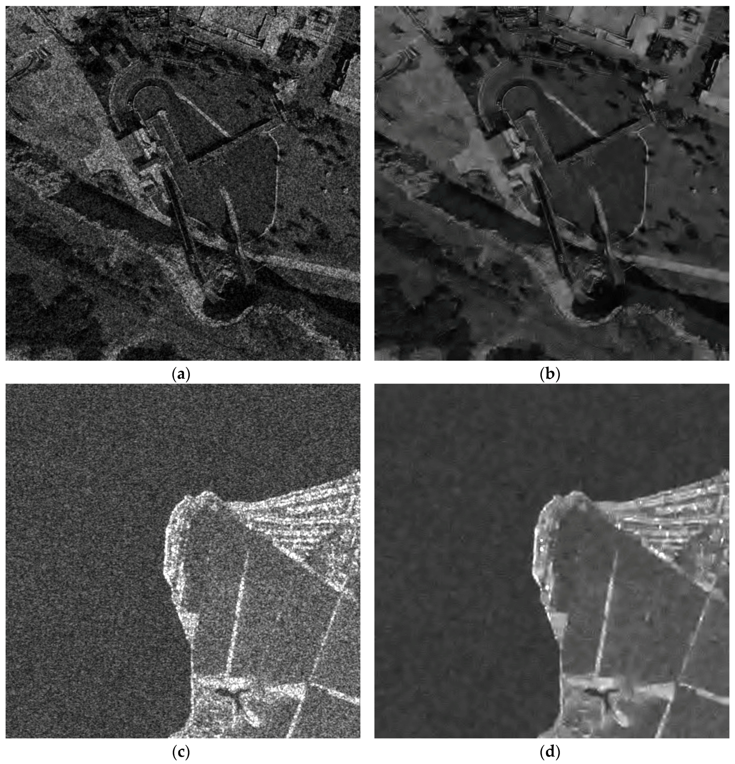
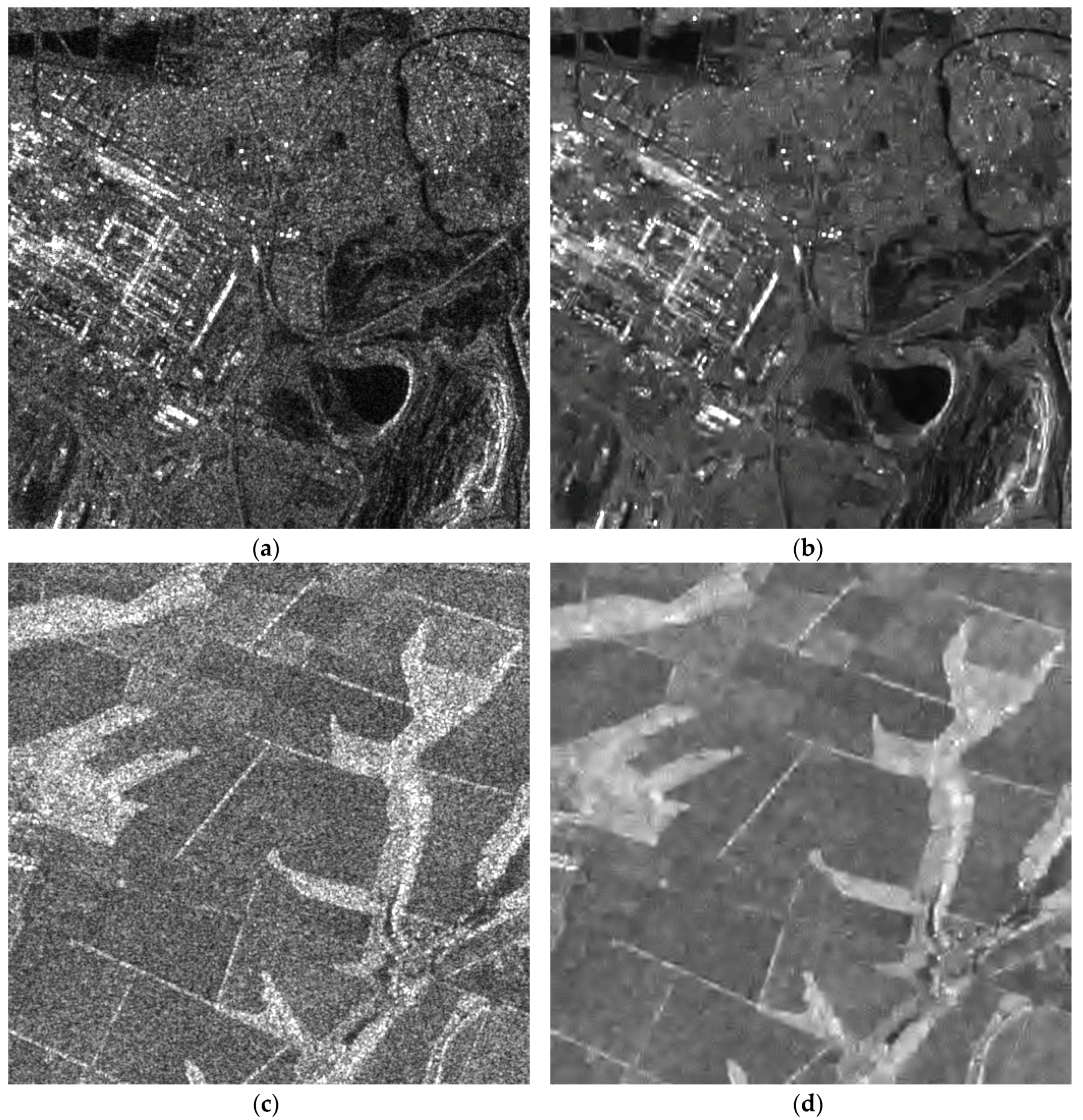
2. Image/Noise Model, Filter and Quality Metrics

Image/noise modelling is based on general knowledge about image and noise properties in SAR images [2,6,7] as well as on information obtained by analysis of real-life Sentinel-1 images [31,45]. A first assumption is that a noise is pure multiplicative. This assumption has been verified practically and proven by using both automatic means as [10] and special tools as ENVI. Experiments have been done for both VV (Vertical-Vertical) and VH (Vertical-Horizontal) polarizations of RS data. The determined (estimated) relative variance of speckle ${\sigma }_{\mu }^2$ is about 0.05 for both polarizations [45]. This approximately corresponds to 5-look amplitude data. As demonstrated in [17], the speckle cannot be “strictly” Gaussian in this case and this has been proven by the Gaussianity tests. However, the speckle probability density function (PDF) is very close to Gaussian.

Figure 1 presents two 512 × 512 pixel fragments of Sentinel-1 dual polarization data with marked manually selected quasi-homogeneous regions with the size of about 190 × 365 pixels. One can see that the speckle is visible, especially in regions with a large mean. However, speckle is practically unnoticeable in regions with low mean values (dark ones) due to a multiplicative nature of noise. Besides, image fragments for different polarizations are quite similar to each other but, certainly, they are not the same.

A fact that the speckle is spatially correlated can be verified in many ways. A typical approach is to analyze a two-dimentional auto-correlation function. Alternatively, one can analyze an estimate of power spectra in DCT domain for 8x8 pixel blocks. To make local estimates insensitive to a local mean, we have calculated normalized power spectral estimates $D_{pn}\left(k,l\right)=D^2\left(k,l\right)/\left(M_{BM}^2{\sigma }_{\mu }^2\right),$ $k=1,\dots ,8;$ $l=1,\dots ,8$ locally (in each considered block, $D\left(k,l\right)$ denotes the $kl$-th DCT coefficient, $M_{BM}$ is the block mean) and averaged the obtained estimates. Small $k$ and $l$ correspond to low spatial frequencies. $D_{pn}\left(1,1\right)$, corresponding to the local mean, is neglected, and the obtained estimate of a normalized spectrum is presented for VV polarization in Figure 2. One can see that low frequencies have larger values of $D_{pn}\left(k,l\right)$ and this clearly shows that the speckle is spatially correlated (for spatially uncorrelated noise the DCT spectrum is close to uniform). The normalized spectrum for other polarization is similar. Expedience of analyzing DCT-spectrum in 8 × 8 pixel blocks will become clear later.

One might wonder that in this paper we concentrate on considering the DCT-based filter adapted to suppress pure multiplicative spatially correlated noise [23,31] while there are numerous filters proposed for this (see [6,7,8,9,10,11,12,13,14,15,16,17,18] and references therein). The reasons for analyzing the DCT-based filter are the following. First, this filter is very simple and fast and can be easily adapted to noise properties (which will be demonstrated below for the considered particular case). Second, this filter has performance comparable to the best known modern filters [24]. Note that to cope with a multiplicative noise, one often has to apply a proper variance-stabilizing transform to provide pre-requisites for applying such filters.

The main stages of DCT-based filtering are the following: perform direct 2D DCT in each block; apply thresholding to DCT-coefficients; perform inverse 2D DCT; aggregate filtering results for overlapping blocks [24,31]. Let us give some details and additional explanations for each stage. Usually blocks of size 8 × 8 pixels are employed (although other variants are possible [17,40]). Different types of thresholding can be applied in block after direct DCT. Below we consider hard locally adaptive frequency dependent thresholding, where a threshold in a given block is set as $T\left(k,l\right)=2.7M_{BM}{\sigma }_{\mu }{D}_{pn}^{0.5}\left(k,l\right)$, i.e., proportionally to the block mean that has to be determined for each block and taking speckle spectrum into account. Hard thresholding is known to be more efficient in terms of conventional criteria of filtering efficiency but it can result in artifacts.

A specific feature of DCT-based filtering is that it is preferable to carry out denoising with block overlapping where full overlapping produces the best efficiency of noise suppression but is slower than processing with partial overlapping (full overlapping means that positions of neighbor blocks differ by only one pixel, e.g., the upper left corner indices are i = 1, j = 1 and i = 2, j = 1; partial overlapping means that positions of neighbor blocks are “shifted” by more pixels, such as i = 1, j = 1 and i = 5, j = 1 for half-overlapping). As the result of filtering in blocks, filtered values are obtained for each pixel of a block. Then, if a given pixel belongs to different blocks, several (up to 64) filtered values are obtained for it. They can be aggregated in different ways, the simplest among them is to average all values.

The DCT-based filter suppresses noise efficiently in homogeneous image regions and preserves texture well enough [17,24]. Meanwhile, its main drawbacks are in smearing high contrast edges and fine details as well as introducing some specific artifacts.

Let’s analyze data for simulated images first where speckle is added artificially. Then, to characterize quality of images and filter performance, it is possible to use full-reference metrics of the following three groups:

• metrics determined for original (noisy) images $\{I_{ij}^n=I_{ij}^{true}{\mu }_{ij},i=1,\dots ,I_{Im};j=1,\dots ,J_{Im}\}$ using available $\{I_{ij}^{true},i=1,\dots ,I_{Im};j=1,\dots ,J_{Im}\}$, where $\{I_{ij}^{true},i=1,\dots ,I_{Im};j=1,\dots ,J_{Im}\}$ denotes the true noise-free image, ${\mu }_{ij}$ defines the speckle in the $ij$-th pixel that has mean equal to unity and variance ${\sigma }_{\mu }^2$, $I_{Im},J_{Im}$ define image size;
• metrics that characterize quality of despeckled images $\{I_{ij}^f,i=1,\dots ,I_{Im};j=1,\dots ,J_{Im}\}$ using available $\{I_{ij}^{true},i=1,\dots ,I_{Im};j=1,\dots ,J_{Im}\}$;
• “improvements” of metric values due to despeckling $IM=M_f-M_{inp}$ where $M_f$ and $M_{inp}$ are metric values for despeckled and original images, respectively.

Such methodology of analysis is explained by the following. First, the quality of original images is important since it shows how actual is the task of image filtering. Recall that in the case of AWGN it has been shown [46] that conventional PSNR about 35 dB corresponds to noise/distortion invisibility threshold under condition that noise/distortions are almost “uniformly” distributed over a considered image. Similarly, visual quality metric PSNR-HVS-M [47] (expressed in dB) has to be about 42 dB or more to correspond to invisibility of noise and distortions. The metric FSIM [29] should be larger than 0.99 to indicate that noise or distortions are practically invisible [46].

Second, quality of output images and metric improvements are important to characterize efficiency of despeckling (denoising). Note that:

• Quality metrics have different ranges of their variation; some of them are expressed in dB [47], other ones vary in the limits from 0 to 1 [29], there exist also metrics [28] that vary in other limits;
• For most metrics, a larger value corresponds to a better quality [29,47] although there are metrics for which smaller values correspond to a better quality [28,48]. This information has to be known before starting analysis using a given metric;
• Many metrics have a “nonlinear” behavior; for example, for the metric FSIM most images have values over 0.8 even if images have a low visual quality. This property complicates analysis;
• Improvement of metric values does not always guarantee that image visual quality has improved; for example, improvement of PSNR by 3…5 dB does not show that image visual quality has improved due to filtering if input PSNR ($PSN{R}_{inp}$) determined for original (noisy) image is low (e.g., about 20 dB); similarly, improvement of FSIM by 0.01 corresponds to sufficient improvement of visual quality if input value of FSIM calculated for original image $FSI{M}_{inp}\approx 0.985$ but the same improvement can correspond to negligible improvement of visual quality if $FSI{M}_{inp}\approx 0.8$.

Thus, in order to use a given metric in analysis, its properties have to be well known in advance. Unfortunately, this is not true for many metrics. In particular, performance of many quality metrics has not been analyzed for the cases of pure multiplicative noise and residual distortions after filtering images originally distorted by speckle.

Keeping this in mind, we carry out further analysis for a limited number of conventional and visual quality metrics. Choosing them from a wide set of available metrics, we have taken into account the following aspects. We deal with denoising single-channel images, thus, metrics intended to assess quality of color images cannot be applied. It is worth considering metrics that have shown themselves to be the best according to results of their verification for large databases (as, e.g., TID2013) or according to results of previous analysis for image denoising applications [49]. Some metrics can be calculated for images represented as 8-bit 2D data arrays whilst others can be determined for images represented in arbitrary range. In this paper, we will present our test images in the range 0–255 and use metrics basically oriented to operate for this range of image representation. We have chosen metrics based on different principles of operation and developed by different research teams.

Therefore, the following metrics are chosen and considered below:

• PSNR and its modification, PSNR-HVS-M [47], that takes into account peculiarities of human vision system (HVS). Both metrics are expressed in dB; larger values correspond to better quality, metric values are positive;
• Visual quality metrics resulted from SSIM, such as FSIM [29], MSSSIM [50], IW-SSIM [51], ADD-SSIM [52], ADD-GSIM [52], SSIM4 [49]. All these metrics vary in the limits from 0 to 1; larger values relate to a higher visual quality;
• Visual quality metric WSNR [53] that is expressed in dB; it has positive values and larger ones relate to better visual quality;
• The recently proposed metric HaarPSI [54] varies from 0 to 1, having larger values for better quality images;
• The visual quality metric GMSD [48] is positive and smaller is better;
• The metric MAD [28] varies in wide limits, is positive and smaller is better;
• The metric GSM [55] varies in narrow limits, is smaller than unity and the larger the better;
• The metric DSS [56] varies in the limits from 0 to 1 and the larger the better.

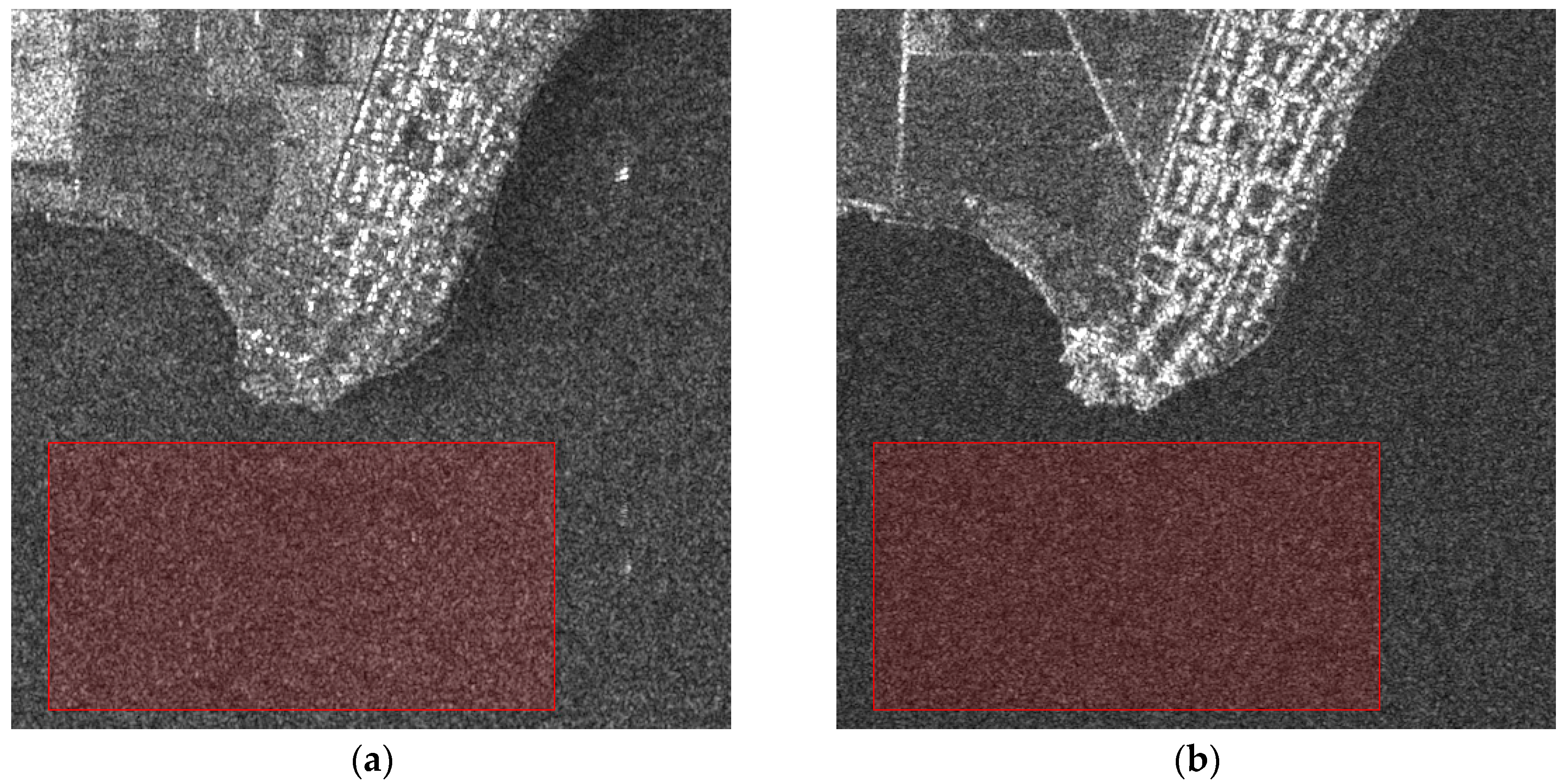
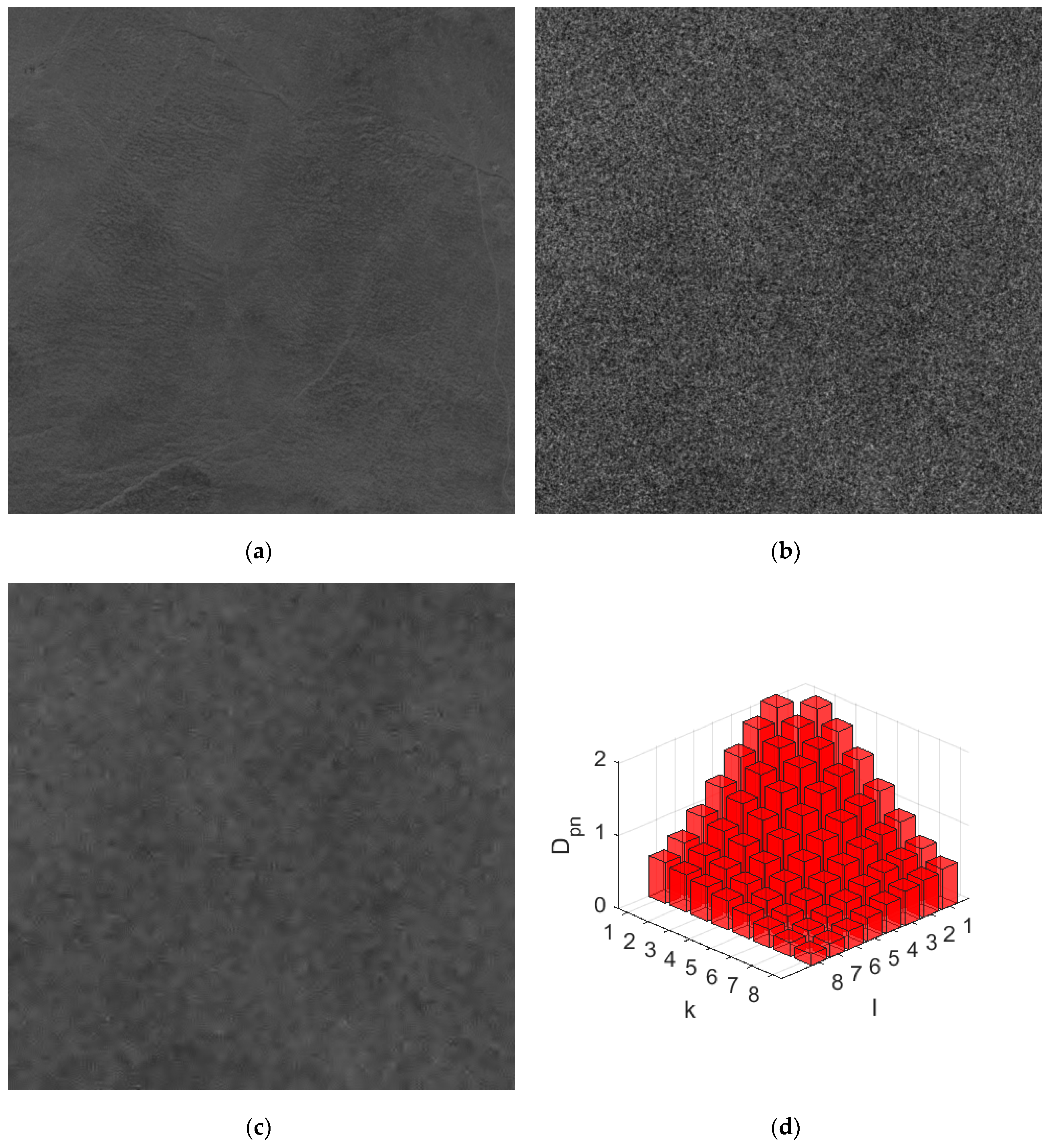
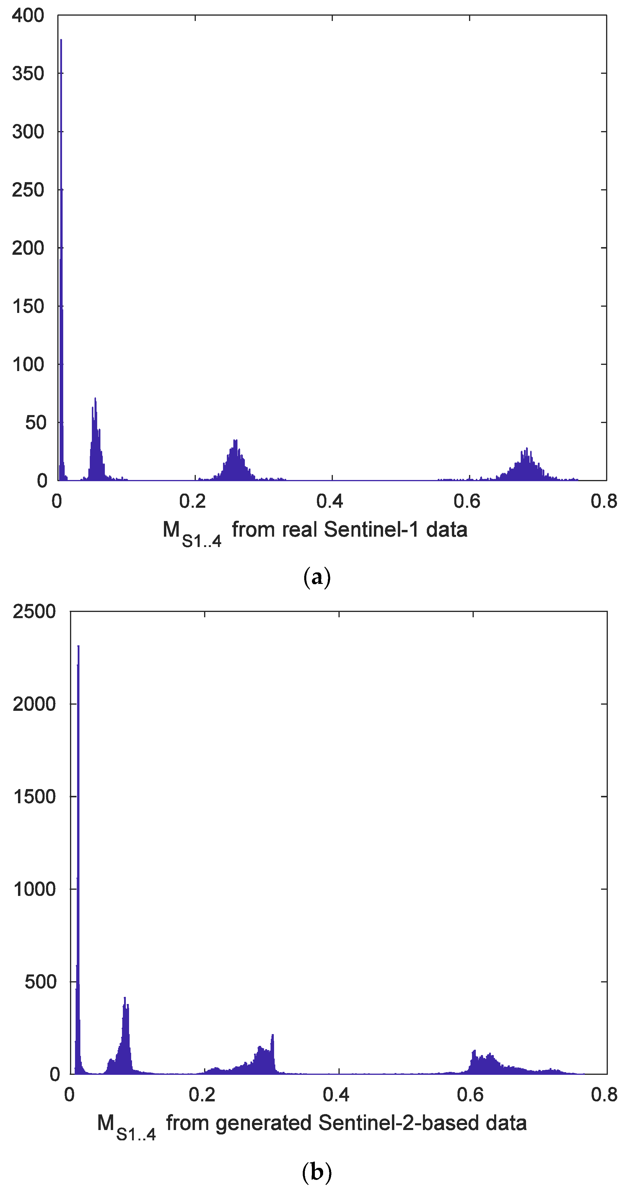
3. Simulated Images and Estimated Parameters

For training a neural network predictor, one requires large number of test images; commonly accepted “true” (noise-free) SAR images are absent. To get around this problem, we have used component images of multispectral RS data that have high SNR with a negligible noise influence. According to analysis in [57], high SNR is observed in channel # 5 of multispectral Sentinel-2 data (freely available). This gives us a large number of test images. One more reason to use optical images as true images is that their fractal properties are similar to fractal properties of radar images of the same terrains.

Having a true image, its noisy version has been obtained using the model given in the previous section. Methodology of modeling spatially correlated noise is described in [19]. To avoid clipping effects after noise is added, original component images of multispectral data have been normalized to the range from 0 to 255.

Examples of noise-free and noisy images are presented in Figure 3a,b. As one can see, noise is intensive and it masks many details and non-intensive texture that can be seen in the true image. The normalized DCT spectrum of the simulated speckle is presented in Figure 3d. Its comparison to the spectrum for real-life images (Figure 2) shows that the main properties of noise spatial correlation are practically the same.

The output image for the DCT-based filter adapted to noise characteristics is given in Figure 3c. It is seen that the filter suppresses the speckle efficiently in image homogeneous regions. The metrics values are the following: noisy PSNR = 23.323 dB, noisy PSNR-HVS-M = 20.484 dB, noisy FSIM = 0.613, IPSNR = 10.256 dB, IPSNR-HVS-M = 9.217 dB, IFSIM = 0.269, but it is unable to retrieve a low intensity texture. Fine detail and edge preservation are worth improving. There are also some denoising artifacts. However, in aggregate, the filter performance is good.

One known problem in NN training and further application is that the training set should correspond to situations that can be met in practice. This means that, at least, the range of input parameter variation has to be approximately the same as for real-life data. Therefore, we have to discuss what parameters can be, at least potentially, used as input parameters.

Earlier we discussed input parameters that are determined in four DCT spectrum areas [38]. A transformed image block in DCT domain is divided into four areas (stripes marked by digits from 1 to 4 in Figure 4). The mark “0” corresponds to the DCT coefficient $D\left(1,1\right)$ with the block mean not “involved” in any area. After this, the following four energy allocation parameters are calculated as

$$W_m=\frac{{{\displaystyle \sum }}_{kl\in A_m}{D}_{kl}^2}{{{\displaystyle \sum }}_{k=1}^8{{\displaystyle \sum }}_{l=1}^8{D}_{kl}^2-D_{11}^2},$$

(1)

where $k$ and $l$ are indices of DCT coefficients in a block ($k=1,\dots ,8; l=1,\dots ,8$), $m$ is an index of the $m$-th area $A_m;$ as one can see, all four values $W$ are in the limits from 0 to 1.

According to [38], four statistical parameters can be determined for $W_m$,$m=1,\dots ,4$, namely, mean, variance, skewness, and kurtosis. Further, they will be denoted as $M_{S1..4}, V_{S1..4}, S_{S1..4}, K_{S1..4}$, respectively, where, e.g., $V_2$ means the variance of $W_2$.

Figure 5 presents the histograms (the number of bins is 1000) of $M_{S1}, M_{S2}, M_{S3},$ and $M_{S4}$ for real-life (Sentinel-1) radar images and for simulated data obtained from high SNR Sentinel-2 images. Values of $M_{S1}$ concentrate around 0.7 whilst values of $M_{S2}, M_{S3}$, and $M_{S4}$ are around 0.26, 0.06, and 0.01, respectively, for Sentinel-1 images (Figure 5a). This relates to the case of spatially correlated noise when the main energy concentrates in low frequency spatial components due to image and noise properties. The histogram in Figure 5b for simulated data is similar to the one in Figure 5a in the sense of its main properties. Histogram peaks are in practically the same places. This means that our model fits the practical case well in the sense of the considered parameters $M_{S1}, M_{S2}, M_{S3},$ and $M_{S4}$. Analysis has been done for other parameters of this group ($V_{S1..4}, S_{S1..4}, K_{S1..4}$) and similar conclusions have been drawn.

The sixteen parameters $M_{S1..4}, V_{S1..4}, S_{S1..4}, K_{S1..4}$ describe the noisy images from the viewpoint of spectral characteristics of noisy images. There are also other types of characteristics that can be exploited. One option is to use image statistics in blocks. These can be parameters $M_{BM}, V_{BM}, S_{BM}, K_{BM}$—mean, variance, skewness, and kurtosis of block means, respectively.

One more group of input parameters that has already recommended itself well in denoising efficiency prediction relates to DCT-coefficient probabilities as the result of their comparison to threshold (or thresholds). Expedience of using such parameters was previously demonstrated [23,24,35]. It has been proposed to analyze the probability that DCT coefficients in blocks do not exceed certain threshold(s). If noise is purely multiplicative and spatially correlated, the algorithm of probability estimation has to be modified appropriately.

In our case, we have estimated $P_{\sigma }\left(q\right), q=1,\dots ,Q$ in the $q$-th block ($Q$ is the total number of analyzed blocks) as

$$P_{\sigma }\left(q\right)=\left({\displaystyle \sum }_{k=1}^8{\displaystyle \sum }_{l=1}^8{\delta }_{qkl}-1\right)/63,$$

(2)

$${\delta }_{qkl}=\{\begin{array}{c}1, if \left|D_q\left(k,l\right)<{\sigma }_{\mu }{\overline{I}}_q{D}_{pn}^{0.5}\left(k,l\right)\right|\\ 0, otherwise\end{array},$$

(3)

where $D_q\left(k,l\right)$ is the $kl$-th DCT coefficient in the $q$-th block, ${\overline{I}}_q$ is the $q$-th block mean.

Having a set of local estimates $P_{\sigma }\left(q\right), q=1,\dots ,Q$, it is possible to calculate the mean, variance, skewness, and kurtosis of this parameter, denoted as $M_P, V_P, S_P, K_P$, respectively. Note that smaller $M_P$ relates to images having a more complex structure (texture or with more details). Here again, we have a good correspondence between histogram shapes and ranges of parameter variation.

Finally, we can expect that image statistics can be useful in quality and filtering efficiency prediction. For this purpose, we have introduced a set of four parameters, namely, image mean, variance, skewness and kurtosis, denoted as $M_I, V_I, S_I, K_I$, respectively. Thus, in total we have 28 statistical parameters that can be used in NN-based prediction.

Note that all parameters that can be used as inputs and allow easy and fast calculation. Additional acceleration deals with the fact [23] that it is usually enough to have about 1000 blocks placed randomly to obtain high accuracy statistics.

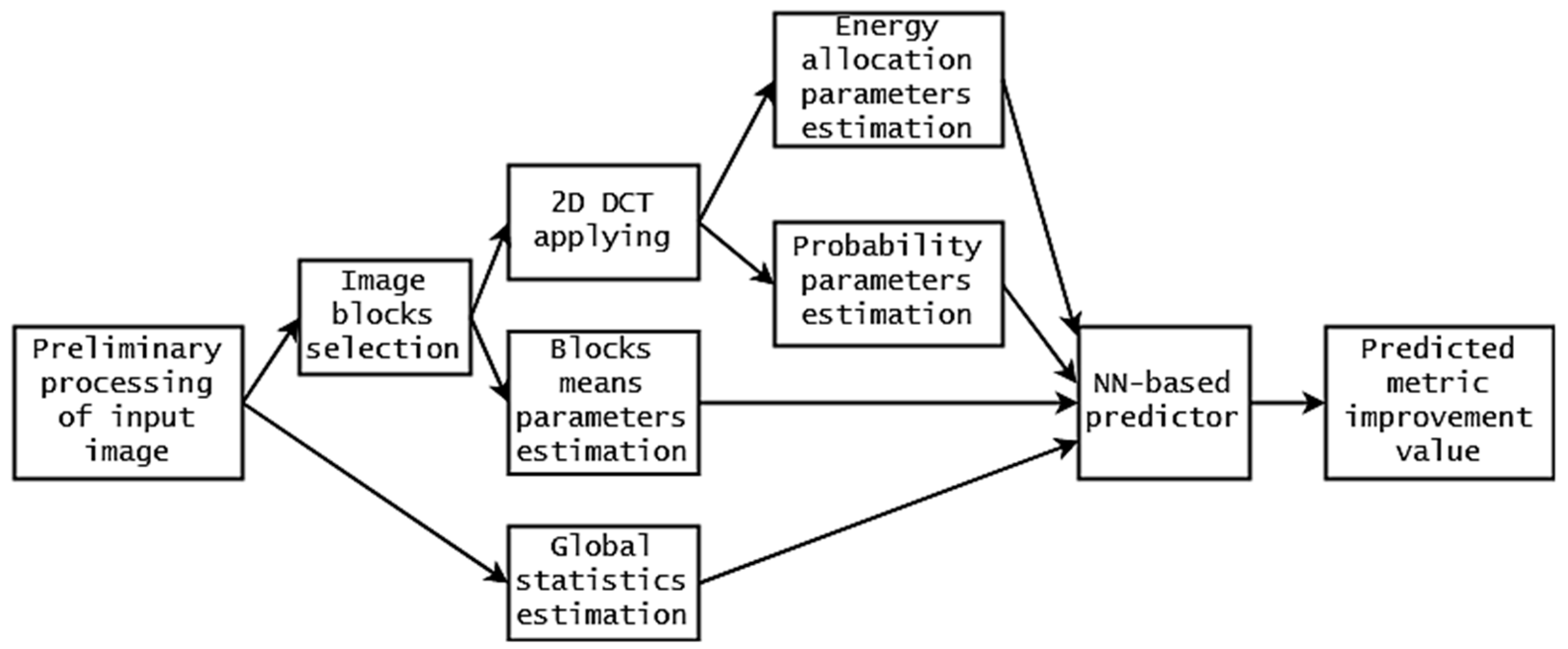
4. Peculiarities of NN Training

As the basic model for denoising efficiency prediction, a feedforward neural network is used. The employed NNs are multilayer all-to-all connected perceptrons that have a common architecture. There are three hidden neuron layers with reducing neuron numbers in each, by two times with respect to the previous layer. The first one has the same number of neurons as the number of input parameters. The second has approximately half of the number of input parameters and the third layer has one quarter of such a number, respectively. For the first two layers, the $tanh$ activation function is exploited. For the third layer, the linear activation function is used. Finally, Bayesian regularization is used as a training function.

Training and verification processes have been divided into four stages. The first two stages deal with self-dataset validation of NNs to find out the optimal set of input parameters, final NN architecture and number of training epochs. The third and fourth stages are carried out to perform cross-dataset evaluation and check the accuracy of trained predictors on data which were not involved in the training process. For the training process, we have used 100 high-quality cloudless multispectral images obtained by Sentinel-2 mission with total sizes about 5500 × 5500 pixels. Due to multispectral features of this data and different levels of distortions present in component images of multispectral data, we have chosen component images in # 5 and # 11 channels with estimated values of PSNR about 50 dB that corresponds to very low intensity of self-noise and high visual quality of images [57]. Data from the channel #5 are related to red edge wavelength that is about 700 nm and data from the channel # 11 corresponds to SWIR where the wavelength is about 1600 nm. These two channels have similar spatial resolution of 20 m. Each image has been divided into smaller images of the size 512 × 512 pixels. Additionally, border parts of original satellite images have been excluded from the dataset collection to avoid defects (like absence of any data) near borders.

In total, we have obtained 8100 test images from each of two channels. Each test image has been corrupted by artificially generated speckle with similar degree of noise spatial correlation and ${\sigma }_{\mu }^2=0.05$ and filtered by the DCT-based filter. For the input noisy images, the metric values and input parameters listed in the previous section that are used for prediction have been estimated. For the denoising outputs, the visual quality metrics values were obtained.

After all data have been collected, we have the following scenario to obtain and verify the NN-based predictors. Self-dataset validation at the first stage has to be performed to establish the most informative input parameters, optimal network architecture and other training process peculiarities. It has been determined that the optimal number of training epochs is 30 for the used NN architecture. For validation, the used dataset has been divided into two parts: 80% for training and 20% for validation. Such operation was repeated for 100 times with full permutation of the dataset for each parameter combination. The obtained RMSE (root mean squared error) and adjusted $R^2$ (coefficient of determination, see below) were averaged to make a decision on final parameter choice.

After optimal combination of input prediction parameters is known, especially for improvement values of all metrics listed above, the final version of predictors for each metrics has to be validated by the same dataset. Unlike the previous stage, the self-dataset validation was carried out 1000 times, and the averaged RMSE and adjusted $R^2$ standard deviations of these criteria are given to prove the stability of the trained NNs using different training and validation datasets. To verify the obtained predictors for images not involved in training process, the cross-dataset evaluation was performed in the following manner. Instead of taking 80 and 20 % of all images (small images cropped from large areas), for this stage, we have divided the dataset in the mentioned proportion for original large size images. This means that we have evaluated the training using 80 large size images taken arbitrarily from the whole dataset, with 20 images left for verification. Similar to the previous stage, the training process was repeated 1000 times for each metric improvement criteria. Note that the described data processing has been carried out using only # 5 channel of Sentinel-2. The last stage deals with cross-dataset evaluation using different large size images and different channels, namely, 80 images from the # 5 channel are taken for training and 20 other images are taken from # 11 channel to check the accuracy of the denoising efficiency prediction. During this stage, we have obtained prediction accuracy results close to real-life image cases like Sentinel-1.

5. Training Results and Verification

In practice, we are interested in providing appropriately accurate prediction with reasonable efforts for obtaining large numbers of input parameters. The maximal number of input parameters in our case is 28, but it is also possible that some parameters described above are non-informative or noise sensitive. It is impossible to consider all possible combinations of input parameters. Besides, it might be so that one combination is good (optimal) for predicting one output parameter whilst another combination offers pre-requisites for predicting another output parameter. Because of this, our trials and analysis are slightly intuitive. In any case, we give the results for trained NN that employs all 28 input parameters but also we present a large number of combinations of input parameters to understand the main trends and tendencies.

Consider first the case of self-validation. The results obtained for predicted improvement of PSNR are given in

Table 1. Data for different combinations of input parameters for prediction of denoising efficiency for I-PSNR.

Combination Number	Input Parameters	RMSE	$\mathbf{Adjusted}{\mathit{R}}^2$
1	$M_{S1..4}$	1.148	0.827
2	$M_{S1..4}$, $V_{S1..4}$	0.939	0.888
3	$M_{S1..4}$, $V_{S1..4}$, $S_{S1..4}$	0.891	0.900
4	$M_{S1..4}$, $V_{S1..4}$, $S_{S1..4}$, $K_{S1..4}$	0.882	0.902
5	$M_{S1..4}$, $M_I$	0.907	0.897
6	$M_{S1..4}$, $V_{S1..4}$, $M_I$	0.791	0.921
7	$M_{S1..4}$, $V_{S1..4}$, $S_{S1..4}$, $M_I$	0.754	0.928
8	$M_{S1..4}$, $V_{S1..4}$, $S_{S1..4}$, $K_{S1..4}$, $M_I$	0.748	0.929
9	$M_{BM}$, $V_{BM}$	1.527	0.703
10	$M_{BM}$, $V_{BM}$, $S_{BM}$	1.469	0.727
11	$M_{BM}$, $V_{BM}$, $S_{BM}$, $K_{BM}$	1.474	0.720
12	$M_P$, $V_P$	1.014	0.861
13	$M_P$, $V_P$, $S_P$	0.929	0.891
14	$M_P$, $V_P$, $S_P$, $K_P$	0.932	0.885
15	$M_I$, $V_I$	1.340	0.769
16	$M_I$, $V_I$, $S_I$	1.296	0.782
17	$M_I$, $V_I$, $S_I$, $K_I$	1.284	0.787
18	$M_{S1..4}$, $M_{BM}$	0.927	0.886
19	$M_{S1..4}$, $M_{BM}$, $M_P$	0.574	0.958
20	$M_{S1..4}$, $M_{BM}$, $M_P$, $M_I$	0.558	0.961
21	$M_{BM}$, $V_{BM}$, $S_{BM}$, $K_{BM}$, $M_I$	1.390	0.757
22	$M_{BM}$, $V_{BM}$, $S_{BM}$, $K_{BM}$, $M_P$, $V_P$, $S_P$, $K_P$	0.555	0.960
23	$M_{BM}$, $V_{BM}$, $S_{BM}$, $K_{BM}$, $M_P$, $V_P$, $S_P$, $K_P$, $M_I$	0.527	0.965
24	$M_{BM}$, $V_{BM}$, $S_{BM}$, $K_{BM}$, $M_P$, $V_P$, $S_P$, $K_P$, $M_I$, $V_I$	0.322	0.986
25	$M_{BM}$, $V_{BM}$, $S_{BM}$, $K_{BM}$, $M_P$, $V_P$, $S_P$, $K_P$, $M_I$, $V_I$, $S_I$	0.303	0.988
26	$M_{BM}$, $V_{BM}$, $S_{BM}$, $K_{BM}$, $M_P$, $V_P$, $S_P$, $K_P$, $M_I$, $V_I$, $S_I$, $K_I$	0.320	0.987
27	$M_{S1..4}$, $M_{BM}$, $V_{BM}$, $S_{BM}$, $K_{BM}$, $M_P$, $V_P$, $S_P$, $K_P$, $M_I$	0.288	0.989
28	$M_{S1..4}$, $M_{BM}$, $V_{BM}$, $S_{BM}$, $K_{BM}$, $M_P$, $V_P$, $S_P$, $K_P$, $M_I$, $V_I$	0.246	0.992
29	$M_{S1..4}$, $M_{BM}$, $V_{BM}$, $S_{BM}$, $K_{BM}$, $M_P$, $V_P$, $S_P$, $K_P$, $M_I$, $V_I$, $S_I$	0.249	0.992
30	$M_{S1..4}$, $M_{BM}$, $V_{BM}$, $S_{BM}$, $K_{BM}$, $M_P$, $V_P$, $S_P$, $K_P$, $M_I$, $V_I$, $S_I$, $K_I$	0.259	0.991
31	$M_{S1..4}$, $V_{S1..4}$, $S_{S1..4}$, $K_{S1..4}$, $M_{BM}$, $V_{BM}$, $S_{BM}$, $K_{BM}$, $M_P$, $V_P$, $S_P$, $K_P$, $M_I$	0.277	0.990
32	$M_{S1..4}$, $M_{BM}$, $V_{BM}$, $S_{BM}$, $K_{BM}$, $M_P$, $V_P$, $S_P$, $K_P$, $M_I$	0.288	0.989
33	$M_{S1..4}$, $M_{BM}$, $V_{BM}$, $S_{BM}$, $M_P$, $V_P$, $S_P$, $K_P$, $M_I$, $V_I$	0.251	0.992
34	$M_{S1..4}$, $M_{BM}$, $V_{BM}$, $S_{BM}$, $M_P$, $V_P$, $S_P$, $K_P$, $M_I$, $V_I$, $S_I$	0.248	0.992
35	$M_{S1..4}$, $M_{BM}$, $V_{BM}$, $S_{BM}$, $M_P$, $V_P$, $S_P$, $K_P$, $M_I$, $V_I$, $S_I$, $K_I$	0.250	0.992
36	$M_{S1..4}$, $V_{S1..4}$, $S_{S1..4}$, $K_{S1..4}$, $M_{BM}$, $V_{BM}$, $S_{BM}$, $K_{BM}$, $M_P$, $V_P$, $S_P$, $K_P$, $M_I$, $V_I$, $S_I$, $K_I$	0.250	0.992

. The data for all 28 input parameters are presented in the last line and the provided RMSE and adjusted $R^2$ [58] are very good—0.25 and 0.992, respectively. Recall that earlier we obtained RMSE and Adjusted $R^2$ about 1.0 and 0.90, respectively, for a simple prediction procedure based on one input parameter in [23]. Thus, the joint use of a large number of input parameters is able to produce considerable benefits.

Let us carry out analysis more in detail. One can see that the use of only four spectral parameters $M_{S1..4}$ (combination # 1) does not provide good results—RMSE = 1.148 and Adjusted $R^2$ is equal to 0.827. The use of other spectral parameters improves the situation—for 16 input parameters (combination # 4), RMSE = 0.882 and Adjusted $R^2$ reaches 0.902. The use of kurtosis parameters does not lead to an essential difference compared to the case when they are not used (combination # 3) RMSE = 0.891 and Adjusted $R^2$ is equal to 0.900. This example shows that some input parameters can be useless.

The use of only one input parameter that describes image statistics ($M_I$) in addition to spectral parameters results in sufficient improvement of prediction accuracy (compare data for combinations ## 5–8 to data for combinations ## 1–4). Statistics of block means used as input parameters without other input parameters (combinations ## 9-11) are non-informative—RMSE is about 1.5 and Adjusted $R^2$ does not exceed 0.72. Probability parameters (combinations ## 12–14) are considerably more informative—the use of four input parameters (combination 14) leads to RMSE = 0.832 and Adjusted $R^2$ is equal to 0.885. It is interesting that the use of kurtosis parameter $K_P$ does not have a positive effect (compare the data for combinations # 14 and # 13).

Parameters that describe image statistics used without other input parameters (combinations ## 15–17) do not produce accurate prediction. However, some combinations that include parameters from different groups (analyze data for combinations ## 18–35) can be very efficient. Among these combinations we can note the following:

• combination # 19 that uses only six input parameters (different means that can be easily calculated) produces RMSE = 0.574 and Adjusted $R^2$ equal to 0.958, i.e., accuracy criteria much better than mentioned above;
• combination # 24 that employs ten input parameters (image statistics and probability parameters) and produces RMSE = 0.322 and Adjusted $R^2$ equal to 0.986, i.e., very good accuracy criteria;
• combination # 33 that involves 13 input parameters that belong to different groups; it provides RMSE = 0.251 and Adjusted $R^2$ equal to 0.992, i.e., the same accuracy as the combination of all 28 input parameters (combination # 36); thus one can choose combination # 33 for practical application if prediction of improvement of PSNR is required.

The results for the self-validation dataset for the metric I-PSNR-HVS-M are given in

Table 2. Data for different combinations of input parameters for prediction of denoising efficiency for I-PSNR-HVS-M.

Combination Number	Input Parameters	RMSE	$\mathbf{Adjusted}{\mathit{R}}^2$
1	$M_{S1..4}$	0.944	0.871
2	$M_{S1..4}$, $V_{S1..4}$	0.793	0.908
3	$M_{S1..4}$, $V_{S1..4}$, $S_{S1..4}$	0.751	0.918
4	$M_{S1..4}$, $V_{S1..4}$, $S_{S1..4}$, $K_{S1..4}$	0.748	0.919
5	$M_{S1..4}$, $M_I$	0.816	0.898
6	$M_{S1..4}$, $V_{S1..4}$, $M_I$	0.656	0.937
7	$M_{S1..4}$, $V_{S1..4}$, $S_{S1..4}$, $M_I$	0.633	0.942
8	$M_{S1..4}$, $V_{S1..4}$, $S_{S1..4}$, $K_{S1..4}$, $M_I$	0.626	0.943
9	$M_{BM}$, $V_{BM}$	1.370	0.729
10	$M_{BM}$, $V_{BM}$, $S_{BM}$	1.364	0.721
11	$M_{BM}$, $V_{BM}$, $S_{BM}$, $K_{BM}$	1.342	0.732
12	$M_P$, $V_P$	1.205	0.790
13	$M_P$, $V_P$, $S_P$	1.180	0.791
14	$M_P$, $V_P$, $S_P$, $K_P$	1.117	0.814
15	$M_I$, $V_I$	1.207	0.786
16	$M_I$, $V_I$, $S_I$	1.175	0.797
17	$M_I$, $V_I$, $S_I,K_I$	1.183	0.790
18	$M_{S1..4}$, $M_{BM}$	0.786	0.911
19	$M_{S1..4}$, $M_{BM}$, $M_P$	0.575	0.952
20	$M_{S1..4}$, $M_{BM}$, $M_P$, $M_I$	0.570	0.953
21	$M_{BM}$, $V_{BM}$, $S_{BM}$, $K_{BM}$, $M_I$	1.266	0.767
22	$M_{BM}$, $V_{BM}$, $S_{BM}$, $K_{BM}$, $M_P$, $V_P$, $S_P$, $K_P$	0.688	0.931
23	$M_{BM}$, $V_{BM}$, $S_{BM}$, $K_{BM}$, $M_P$, $V_P$, $S_P$, $K_P$, $M_I$	0.666	0.935
24	$M_{BM}$, $V_{BM}$, $S_{BM}$, $K_{BM}$, $M_P$, $V_P$, $S_P$, $K_P$, $M_I$, $V_I$	0.370	0.980
25	$M_{BM}$, $V_{BM}$, $S_{BM}$, $K_{BM}$, $M_P$, $V_P$, $S_P$, $K_P$, $M_I$, $V_I$, $S_I$	0.357	0.981
26	$M_{BM}$, $V_{BM}$, $S_{BM}$, $K_{BM}$, $M_P$, $V_P$, $S_P$, $K_P$, $M_I$, $V_I$, $S_I$, $K_I$	0.375	0.979
27	$M_{S1..4}$, $M_{BM}$, $V_{BM}$, $S_{BM}$, $K_{BM}$, $M_P$, $V_P$, $S_P$, $K_P$, $M_I$	0.302	0.987
28	$M_{S1..4},M_{BM},V_{BM},S_{BM},K_{BM}, M_P,V_P,S_P,K_P,M_I,V_I$	0.264	0.990
29	$M_{S1..4},M_{BM},V_{BM},S_{BM},K_{BM}, M_P,V_P,S_P,K_P,M_I,V_I,S_I$	0.263	0.990
30	$M_{S1..4},M_{BM},V_{BM},S_{BM},K_{BM}, M_P,V_P,S_P,K_P,M_I,V_I,S_I,K_I$	0.264	0.990
31	$M_{S1..4}$, $V_{S1..4}$, $S_{S1..4}$, $K_{S1..4}$, $M_{BM}$, $V_{BM}$, $S_{BM}$, $K_{BM}$, $M_P$, $V_P$, $S_P,K_P$, $M_I$	0.290	0.988
32	$M_{S1..4}$, $M_{BM}$, $V_{BM}$, $S_{BM}$, $K_{BM}$, $M_P$, $V_P$, $S_P$, $K_P$, $M_I$	0.300	0.987
33	$M_{S1..4}$, $M_{BM}$, $V_{BM}$, $S_{BM}$, $M_P$, $V_P$, $S_P$, $K_P$, $M_I$, $V_I$	0.272	0.989
34	$M_{S1..4}$, $M_{BM}$, $V_{BM}$, $S_{BM}$, $M_P$, $V_P$, $S_P$, $K_P$, $M_I$, $V_I$, $S_I$	0.268	0.989
35	$M_{S1..4}$, $M_{BM}$, $V_{BM}$, $S_{BM}$, $M_P$, $V_P$, $S_P$, $K_P$, $M_I$, $V_I$, $S_I$, $K_I$	0.262	0.990
36	$M_{S1..4}$, $V_{S1..4}$, $S_{S1..4}$, $K_{S1..4}$, $M_{BM}$, $V_{BM}$, $S_{BM}$, $K_{BM}$, $M_P$, $V_P$, $S_P$, $K_P$, $M_I$, $V_I$, $S_I$, $K_I$	0.263	0.990

. The most important observation is that RMSE about 0.26 and an Adjusted R² of 0.990 can be reached (see data for combinations ## 33–36 in Table 2). Such accuracy has not been gained in our previous studies and its improvement is sufficient. Another important observation is that there is no necessity to use all 28 input parameters—for combination # 34, only 14 input parameters are employed whilst combination # 35 involves 15 input parameters. Note that both combinations include all four parameters that characterize probabilities ($M_P$, $V_P$, $S_P$, $K_P$). Other combinations to be selected are # 19 and 20 with only six and seven input parameters, respectively. Again, the joint use of parameters that belong to different groups provides benefits. This is explained by the fact that these features characterize a processed image from different viewpoints and this is just the case when neural networks beneficially exploit advantages of different input parameters (features). Combination # 33 is very good.

Consider now improvement prediction for the recently proposed visual quality metric SSIM4 [49]. The results are presented in

Table 3. Data for different combinations of input parameters for prediction of denoising efficiency for I-SSIM4.

Combination Number	Input Parameters	RMSE	$\mathbf{Adjusted}{\mathit{R}}^2$
1	$M_{S1..4}$	0.081	0.846
2	$M_{S1..4}$, $V_{S1..4}$	0.067	0.898
3	$M_{S1..4}$, $V_{S1..4}$, $S_{S1..4}$	0.063	0.910
4	$M_{S1..4}$, $V_{S1..4}$, $S_{S1..4}$, $K_{S1..4}$	0.063	0.911
5	$M_{S1..4}$, $M_I$	0.055	0.921
6	$M_{S1..4}$, $V_{S1..4}$, $M_I$	0.043	0.958
7	$M_{S1..4}$, $V_{S1..4}$, $S_{S1..4}$, $M_I$	0.043	0.958
8	$M_{S1..4}$, $V_{S1..4}$, $S_{S1..4}$, $K_{S1..4}$, $M_I$	0.042	0.960
9	$M_{BM}$, $V_{BM}$	0.109	0.730
10	$M_{BM}$, $V_{BM}$, $S_{BM}$	0.104	0.754
11	$M_{BM}$, $V_{BM}$, $S_{BM},K_{BM}$	0.101	0.768
12	$M_P$, $V_P$	0.103	0.753
13	$M_P$, $V_P$, $S_P$	0.097	0.777
14	$M_P$, $V_P$, $S_P$, $K_P$	0.092	0.808
15	$M_I$, $V_I$	0.093	0.805
16	$M_I$, $V_I$, $S_I$	0.089	0.815
17	$M_I$, $V_I$, $S_I$, $K_I$	0.091	0.800
18	$M_{S1..4}$, $M_{BM}$	0.052	0.937
19	$M_{S1..4}$, $M_{BM}$, $M_P$	0.036	0.964
20	$M_{S1..4}$, $M_{BM}$, $M_P$, $M_I$	0.034	0.975
21	$M_{BM}$, $V_{BM}$, $S_{BM}$, $K_{BM}$, $M_I$	0.098	0.786
22	$M_{BM}$, $V_{BM}$, $S_{BM}$, $K_{BM}$, $M_P$, $V_P$, $S_P$, $K_P$	0.057	0.926
23	$M_{BM}$, $V_{BM}$, $S_{BM}$, $K_{BM}$, $M_P$, $V_P$, $S_P$, $K_P$, $M_I$	0.056	0.924
24	$M_{BM}$, $V_{BM}$, $S_{BM}$, $K_{BM}$, $M_P$, $V_P$, $S_P$, $K_P$, $M_I$, $V_I$	0.029	0.980
25	$M_{BM}$, $V_{BM}$, $S_{BM}$, $K_{BM}$, $M_P$, $V_P$, $S_P$, $K_P$, $M_I$, $V_I$, $S_I$	0.028	0.981
26	$M_{BM}$, $V_{BM}$, $S_{BM}$, $K_{BM}$, $M_P$, $V_P$, $S_P$, $K_P$, $M_I$, $V_I$, $S_I$, $K_I$	0.030	0.979
27	$M_{S1..4}$, $M_{BM}$, $V_{BM}$, $S_{BM}$, $K_{BM}$, $M_P$, $V_P$, $S_P$, $K_P$, $M_I$	0.020	0.991
28	$M_{S1..4}$, $M_{BM}$, $V_{BM}$, $S_{BM}$, $K_{BM}$, $M_P$, $V_P$, $S_P$, $K_P$, $M_I$, $V_I$	0.019	0.992
29	$M_{S1..4}$, $M_{BM}$, $V_{BM}$, $S_{BM}$, $K_{BM}$, $M_P$, $V_P$, $S_P$, $K_P$, $M_I$, $V_I$, $S_I$	0.019	0.992
30	$M_{S1..4}$, $M_{BM}$, $V_{BM}$, $S_{BM}$, $K_{BM}$, $M_P$, $V_P$, $S_P$, $K_P$, $M_I$, $V_I$, $S_I$, $K_I$	0.019	0.992
31	$M_{S1..4}$, $V_{S1..4}$, $S_{S1..4}$, $K_{S1..4}$, $M_{BM}$, $V_{BM}$, $S_{BM}$, $K_{BM}$, $M_P$, $V_P$, $S_P$, $K_P$, $M_I$	0.018	0.993
32	$M_{S1..4}$, $M_{BM}$, $V_{BM}$, $S_{BM}$, $K_{BM}$, $M_P$, $V_P$, $S_P$, $K_P$, $M_I$	0.020	0.991
33	$M_{S1..4}$, $M_{BM}$, $V_{BM}$, $S_{BM}$, $M_P$, $V_P$, $S_P$, $K_P$, $M_I$, $V_I$	0.019	0.992
34	$M_{S1..4}$, $M_{BM}$, $V_{BM}$, $S_{BM}$, $M_P$, $V_P$, $S_P$, $K_P$, $M_I$, $V_I$, $S_I$	0.019	0.992
35	$M_{S1..4}$, $M_{BM}$, $V_{BM}$, $S_{BM}$, $M_P$, $V_P$, $S_P$, $K_P$, $M_I$, $V_I$, $S_I$, $K_I$	0.019	0.992
36	$M_{S1..4}$, $V_{S1..4}$, $S_{S1..4}$, $K_{S1..4}$, $M_{BM}$, $V_{BM}$, $S_{BM}$, $K_{BM}$, $M_P$, $V_P$, $S_P$, $K_P$, $M_I$, $V_I$, $S_I$, $K_I$	0.019	0.992

. For all 36 input parameters used jointly, a very good result is observed—RMSE = 0.019 and Adjusted $R^2$ is equal to 0.992 (recall here that SSIM4 varies within the limits from 0 to 1). A practically important advantage is that it is possible to apply fewer input parameters (combinations ## 33–35) to produce the same accuracy. Again, we can note combinations # 19 and 20 that employ only six and seven input parameters, respectively.

Aggregating the obtained results, we can state that combination # 33 produces excellent prediction for all three considered metrics (see data in Table 1, Table 2 and Table 3) that correspond to different groups (conventional metric, visual quality metric of DCT-based family, visual quality metric of SSIM-based family). The block diagram presenting the operations undertaken is shown in Figure 6. Table 1, Table 2 and Table 3 give the results of average RMSE and Adjusted $R^2$ for 100 realizations of NN learning. Sometime, training results can sufficiently differ for different realizations. To show that training is stable,

Table 4. Self-dataset validation in the same channel (# 5).

Output Parameters	RMSE	STD of RMSE	$\mathbf{Adjusted}{\mathit{R}}^2$	$\mathbf{STD}\mathbf{of}\mathbf{Adjusted}{\mathit{R}}^2$
I-PSNR	0.251	0.027	0.992	0.002
I-PSNRHVSM	0.264	0.024	0.990	0.002
I-FSIM	0.018	0.001	0.982	0.003
I-MSSSIM	0.010	0.001	0.994	0.001
I-GMSD	0.011	0.001	0.953	0.007
I-HaarPSI	0.020	0.001	0.972	0.004
I-GSM	0.002	0.000	0.991	0.001
I-SSIM4	0.019	0.002	0.992	0.002
I-MAD	3.620	0.252	0.894	0.014
I-IWSSIM	0.015	0.001	0.979	0.003
I-ADDSSIM	0.001	0.000	0.962	0.005
I-ADDGSIM	0.001	0.000	0.956	0.007
I-DSS	0.034	0.002	0.945	0.007
I-WSNR	0.198	0.017	0.988	0.002

presents mean and standard deviation (STD) data for RMSE and Adjusted $R^2$ for 1000 realizations of NN training. As one can see, the STD of RMSE is always one order less than RMSE. STD values of Adjusted $R^2$ are small, and this shows that training produces stable results.

The most important observation is that Adjusted $R^2$ is very large for most metrics. There are many metrics for which Adjusted $R^2$ is about 0.99. For some metrics such as GMSD, HaarPSI, IWSSIM, ADDSSIM, ADDGSIM, DSS, the obtained results are good enough and only for the metric I-MAD is the prediction accuracy worth improving. The results that are presented in Table 4 can be roughly compared to the data in Table 1 (left part) in the paper [38]. Here, we say “roughly” because an additive noise case is studied in the paper [38]. Comparison shows that the provided RMSE and Adjusted $R^2$ for the proposed NN predictor that employs not only spectral but also other parameters are sufficiently better. In our opinion, this is attributed to a joint use of input parameters that relate to different groups and to taking into account noise characteristics that take place for images acquired by Sentinel-1.

Sometimes characteristics of NN-based predictors and classifiers become radically worse if they are trained for one set of data and applied to another set of data. To check performance of the designed NN-based predictor, we have carried out cross-validations, i.e., have performed training for 6480 test images and estimated accuracy parameters for other 1620 images. The results are given in

Table 5. Cross-dataset evaluation in the same channel (# 5).

Output Parameters	RMSE	STD of RMSE	$\mathbf{Adjusted}{\mathit{R}}^2$	$\mathbf{STD}\mathbf{of}\mathbf{Adjusted}{\mathit{R}}^2$
I-PSNR	0.271	0.036	0.990	0.003
I-PSNRHVSM	0.285	0.042	0.987	0.006
I-FSIM	0.019	0.002	0.978	0.007
I-MSSSIM	0.011	0.002	0.993	0.003
I-GMSD	0.012	0.002	0.939	0.037
I-HaarPSI	0.022	0.004	0.964	0.032
I-GSM	0.002	0.000	0.989	0.004
I-SSIM4	0.021	0.002	0.990	0.003
I-MAD	3.999	0.844	0.865	0.046
I-IWSSIM	0.016	0.002	0.973	0.009
I-ADDSSIM	0.001	0.000	0.952	0.016
I-ADDGSIM	0.002	0.000	0.944	0.023
I-DSS	0.037	0.004	0.932	0.017
I-WSNR	0.214	0.026	0.986	0.004

. They can be compared to the corresponding data in Table 4. As one can see, the results have become worse, but not much. RMSE values have increased by 5–10 %, and Adjusted $R^2$ values have decreased slightly. However, in general, the accuracy is still very high for almost all considered metrics.

Finally, one more verification of the method’s accuracy has been employed. As mentioned above, data from channel # 5 of Sentinel-2 images have been used in training. We have carried out cross-validation using test images with simulated speckle using images in channel # 11 of Sentinel-2. The obtained results are given in

Table 6. Cross-dataset evaluation using another channel (# 11).

Output Parameters	RMSE	STD of RMSE	$\mathbf{Adjusted}{\mathit{R}}^2$	$\mathbf{STD}\mathbf{of}\mathbf{Adjusted}{\mathit{R}}^2$
I-PSNR	0.417	0.070	0.965	0.016
I-PSNRHVSM	0.429	0.071	0.962	0.015
I-FSIM	0.023	0.002	0.958	0.016
I-MSSSIM	0.014	0.002	0.986	0.005
I-GMSD	0.018	0.002	0.868	0.043
I-HaarPSI	0.031	0.004	0.921	0.024
I-GSM	0.003	0.001	0.975	0.032
I-SSIM4	0.030	0.003	0.975	0.008
I-MAD	4.764	0.799	0.744	0.085
I-IWSSIM	0.019	0.002	0.957	0.013
I-ADDSSIM	0.002	0.000	0.882	0.043
I-ADDGSIM	0.002	0.000	0.812	0.083
I-DSS	0.050	0.006	0.873	0.039
I-WSNR	0.311	0.049	0.963	0.013

. RMSE values have increased and Adjusted $R^2$ has decreased although they are still good for most of the considered metrics except GMSD, MAD, ADDSSIM, ADDGSIM, and DSS.

Prediction results can be also verified in other ways. Noisy input data and the denoising outputs for the FRTest#2 image (earlier used in analysis of despeckling efficiency in [23])) and real-life image acquired by Sentinel-1 are presented in Figure 7. The first image has been corrupted by noise of the model with the parameters corresponding to parameters of speckle in Sentinel-1 data. The values of some metrics for the input noisy image are the following: PSNR = 24.842 dB, PSNR-HVS-M = 22.353 dB and FSIM = 0.848. The obtained denoising results expressed by improvements of the used metrics are 4.414 dB, 3.722 dB and 0.059, respectively. The predicted values of the corresponding improvements of aforementioned metrics are 4.303 dB, 3.697 dB and 0.045. As one can see, the differences are very small, i.e., prediction is accurate.

The second image was cropped from the Sentinel-1 image and has been treated by the proposed approach without a priori known metrics values of input data and achievable improvement of visual quality. The obtained results of prediction are 11.841 dB, 10.779 dB and 0.344 for I-PSNR, I-PSNR-HVS, and I-FSIM, respectively. It is impossible to get the true values of improvements since the noise-free image is absent. The predicted metric values are large and correspond to considerable improvement of image quality due to despeckling. This is in good agreement with visual inspection. Speckle is sufficiently suppressed in large homogeneous regions whilst edges and fine details are well preserved.

Figure 8 shows the marginal results of minimal and maximal predicted values of I-PSNR after the trained NN has been applied to Sentinel-1 images. The minimal predicted value corresponds to a low-intensity image where the signal-dependent noise has a low level and visual quality is appropriate (Figure 8a). There are high contrast objects and edges here that restrict denoising efficiency. As a result, the predicted improvement is not too high, although noticeable, and fine details are well preserved. The maximal predicted I-PSNR corresponds to a high-intensity image with the set of large sized homogenous regions (presumably crop fields). The improvement, according to visual inspection, is quite large although there are some rudimentary low-frequency distortions caused by the spatially correlated nature of the speckle.

6. Conclusions

Modern SAR systems produce enormous amounts of data. Sentinel-1 is one of such system, and images acquired by this system have already found many applications. As for any SAR data, the speckle is the factor that prevents their more efficient use, and removal of the speckle remains an important task. Having many methods at disposal, users still run into situations when despeckling is not efficient enough or even useless. Then, it is reasonable to have predictors of filtering efficiency for a given image fragment and for a given filter. We have considered one of the best despeckling algorithms based on a sliding window DCT adapted to multiplicative nature of the noise and its spatial correlation. For this filter, it is shown that many metrics, both traditional and unconventional (visual quality ones), can be predicted using a set of quite simple statistical parameters used as inputs of the trained neural network having a rather simple structure. Several quasi-optimal sets of input parameters are obtained. Source code and data samples are provided as Supplementary Materials.

Data simulation and training peculiarities are considered in detail because of the absence of model SAR data and true images. It is shown that the obtained models are accurate and they allow predicting many metrics with high accuracy. This high accuracy is proven in different ways using self-validation, cross-validation and real-life data analysis. The obtained RMSE values are several times smaller than those ones obtained in earlier research. Other advantages of the proposed approach are demonstrated.

In the future, it is desirable to carry out experiments with experts in visual analysis of SAR images to get their opinions on when image despeckling is expedient. It is also worth analyzing other types of despeckling methods.

References

1. Schowengerdt, R.A. Remote Sensing: Models and Methods for Image Processing, 3rd ed.; Academic Press: San Diego, CA, USA, 2007. [Google Scholar]
2. Lee, J.S.; Pottier, E. Polarimetric Radar Imaging: From Basics to Applications; CRC Press: Boca Raton, FL, USA, 2009; p. 422. [Google Scholar]
3. Kussul, N.; Skakun, S.; Shelestov, A.; Kussul, O. The use of satellite SAR imagery to crop classification in Ukraine within JECAM project. In Proceedings of the IEEE International Geoscience and Remote Sensing Symposium (IGARSS), Quebec, QC, Canada, 13–18 July 2014; pp. 1497–1500. [Google Scholar] [CrossRef]
4. Roth, A.; Marschalk, U.; Winkler, K.; Schättler, B.; Huber, M.; Georg, I.; Künzer, C.; Dech, S. Ten Years of Experience with Scientific TerraSAR-X Data Utilization. Remote Sens. 2018, 10, 1170. [Google Scholar] [CrossRef]
5. Mullissa, A.G.; Persello, C.; Tolpekin, V. Fully Convolutional Networks for Multi-Temporal SAR Image Classification. In Proceedings of the IEEE International Geoscience and Remote Sensing Symposium, Valencia, Spain, 22–27 July 2018; pp. 6635–6638. [Google Scholar] [CrossRef]
6. Oliver, C.; Quegan, S. Understanding Synthetic Aperture Radar Images; SciTech Publishing: Raleigh, NC, USA, 2004. [Google Scholar]
7. Touzi, R. Review of Speckle Filtering in the Context of Estimation Theory. IEEE Trans. Geosci. Remote Sens. 2002, 40, 2392–2404. [Google Scholar] [CrossRef]
8. Kupidura, P. Comparison of Filters Dedicated to Speckle Suppression in SAR Images. Int. Arch. Photogramm. Remote Sens. Spat. Inf. Sci. 2016, XLI–B7, 269–276. [Google Scholar] [CrossRef]
9. Vasile, G.; Trouvé, E.; Lee, J.S.; Buzuloiu, V. Intensity-driven adaptive-neighborhood technique for polarimetric and interferometric SAR parameters estimation. IEEE Trans. Geosci. Remote Sens. 2006, 44, 1609–1621. [Google Scholar] [CrossRef] [Green Version]
10. Anfinsen, S.N.; Doulgeris, A.P.; Eltoft, T. Estimation of the Equivalent Number of Looks in Polarimetric SAR Imagery. In Proceedings of the IEEE International Geoscience and Remote Sensing Symposium, Boston, MA, USA, 7–11 July 2008; pp. 487–490. [Google Scholar] [CrossRef]
11. Deledalle, C.; Denis, L.; Tabti, S.; Tupin, F. MuLoG, or how to apply Gaussian denoisers to multi-channel SAR speckle reduction? IEEE Trans. Image Process. 2017, 26, 4389–4403. [Google Scholar] [CrossRef] [PubMed]
12. Solbo, S.; Eltoft, T. A stationary wavelet domain Wiener filter for correlated speckle. IEEE Trans. Geosci. Remote Sens. 2008, 46, 1219–1230. [Google Scholar] [CrossRef]
13. Lee, J.S.; Wen, J.H.; Ainsworth, T.; Chen, K.S.; Chen, A. Improved Sigma Filter for Speckle Filtering of SAR Imagery. IEEE Trans. Geosci. Remote Sens. 2009, 47, 202–213. [Google Scholar] [CrossRef]
14. Parrilli, S.; Poderico, M.; Angelino, C.; Verdoliva, L. A nonlocal SAR image denoising algorithm based on LLMMSE wavelet shrinkage. IEEE Trans. Geosci. Remote Sens. 2012, 50, 606–616. [Google Scholar] [CrossRef]
15. Yun, S.; Woo, H. A new multiplicative denoising variational model based on mth root transformation. IEEE Trans. Image Process. 2012, 21, 2523–2533. [Google Scholar] [CrossRef]
16. Makitalo, M.; Foi, A.; Fevralev, D.; Lukin, V. Denoising of single-look SAR images based on variance stabilization and non-local filters. In Proceedings of the International Conference on Mathematical Methods in Electromagnetic Theory (MMET), Kiev, Ukraine, 6–8 September 2010; pp. 1–4. [Google Scholar] [CrossRef]
17. Tsymbal, O.; Lukin, V.; Ponomarenko, N.; Zelensky, A.; Egiazarian, K.; Astola, J. Three-state locally adaptive texture preserving filter for radar and optical image processing. EURASIP J. Appl. Signal Process. 2005, 2005, 1185–1204. [Google Scholar] [CrossRef]
18. Deledalle, C.; Tupin, F.; Denis, L. Patch similarity under non Gaussian noise. In Proceedings of the IEEE International Conference on Image Processing (ICIP), Brussels, Belgium, 11–14 September 2011; pp. 1885–1888. [Google Scholar] [CrossRef]
19. Rubel, O.; Lukin, V.; Egiazarian, K. Additive Spatially Correlated Noise Suppression by Robust Block Matching and Adaptive 3D Filtering. J. Imaging Sci. Technol. 2018, 62, 6040-1–6040-11. [Google Scholar] [CrossRef]
20. Fevralev, D.; Lukin, V.; Ponomarenko, N.; Abramov, S.; Egiazarian, K.; Astola, J. Efficiency analysis of color image filtering. EURASIP J. Adv. Signal Process. 2011, 2011, 1–19. [Google Scholar] [CrossRef]
21. Chatterjee, P.; Milanfar, P. Is Denoising Dead? IEEE Trans. Image Process. 2010, 19, 895–911. [Google Scholar] [CrossRef] [PubMed]
22. Chatterjee, P.; Milanfar, P. Practical Bounds on Image Denoising: From Estimation to Information. IEEE Trans. Image Process. 2011, 20, 1221–1233. [Google Scholar] [CrossRef] [PubMed]
23. Rubel, O.; Lukin, V.; de Medeiros, F. Prediction of Despeckling Efficiency of DCT-based filters Applied to SAR Images. In Proceedings of the International Conference on Distributed Computing in Sensor Systems, Fortaleza, Brazil, 10–12 June 2015; pp. 159–168. [Google Scholar] [CrossRef]
24. Rubel, O.; Abramov, S.; Lukin, V.; Egiazarian, K.; Vozel, B.; Pogrebnyak, A. Is Texture Denoising Efficiency Predictable? Int. J. Pattern Recognit. Artif. Intell. 2018, 32, 1860005. [Google Scholar] [CrossRef]
25. Singh, P.; Shree, R. A new SAR image despeckling using directional smoothing filter and method noise thresholding. Eng. Sci. Technol. Int. J. 2018, 21, 589–610. [Google Scholar] [CrossRef]
26. Wang, P.; Patel, V. Generating high quality visible images from SAR images using CNNs. In Proceedings of the IEEE Radar Conference (RadarConf18), Oklahoma City, OK, USA, 23–27 April 2018; pp. 570–575. [Google Scholar] [CrossRef]
27. Gomez, L.; Ospina, R.; Frery, A.C. Statistical Properties of an Unassisted Image Quality Index for SAR Imagery. Remote Sens. 2019, 11, 385. [Google Scholar] [CrossRef]
28. Larson, E.; Chandler, D. Most apparent distortion: Full-reference image quality assessment and the role of strategy. J. Electron. Imaging 2010, 19, 011006:1–011006:21. [Google Scholar] [CrossRef]
29. Zhang, L.; Zhang, L.; Mou, X.; Zhang, D. FSIM: A feature similarity index for image quality assessment. IEEE Trans. Image Process. 2011, 20, 2378–2386. [Google Scholar] [CrossRef]
30. SENTINEL-1 SAR User Guide Introduction. Available online: https://sentinel.esa.int/web/sentinel/user-guides/sentinel-1-sar (accessed on 4 April 2019).
31. Lopez-Martinez, C.; Lopez-Sanchez, J.M. Special Issue on Polarimetric SAR Techniques and Applications. Appl. Sci. 2017, 7, 768. [Google Scholar] [CrossRef]
32. Abdikan, S.; Sanli, F.; Ustuner, M.; Calò, F. Land Cover Mapping Using Sentinel-1 SAR Data. Int. Arch. Photogramm. Remote Sens. Spat. Inf. Sci. 2016, XLI–B7, 757–761. [Google Scholar] [CrossRef]
33. Whelen, T.; Siqueira, P. Time-series classification of Sentinel-1 agricultural data over North Dakota. Remote Sens. Lett. 2018, 9, 411–420. [Google Scholar] [CrossRef]
34. Abramov, S.; Krivenko, S.; Roenko, A.; Lukin, V.; Djurovic, I.; Chobanu, M. Prediction of Filtering Efficiency for DCT-based Image Denoising. In Proceedings of the Mediterranean Conference on Embedded Computing (MECO), Budva, Serbia, 15–20 June 2013; pp. 97–100. [Google Scholar] [CrossRef]
35. Lukin, V.; Abramov, S.; Kozhemiakin, R.; Rubel, A.; Uss, M.; Ponomarenko, N.; Abramova, V.; Vozel, B.; Chehdi, K.; Egiazarian, K.; et al. DCT-Based Color Image Denoising: Efficiency Analysis and Prediction. In Color Image and Video Enhancement; Emre Celebi, M., Lecca, M., Smolka, B., Eds.; Springer International Publishing: Cham, Switzerland, 2015; pp. 55–80. [Google Scholar]
36. Rubel, A.; Lukin, V.; Egiazarian, K. A method for predicting DCT-based denoising efficiency for grayscale images corrupted by AWGN and additive spatially correlated noise. In Proceedings of the SPIE Conference Image Processing: Algorithms and Systems XIII, San Francisco, CA, USA, 10–11 February 2015; Volume 9399. [Google Scholar] [CrossRef]
37. Rubel, A.; Rubel, O.; Lukin, V. On Prediction of Image Denoising Expedience Using Neural Networks. In Proceedings of the International Scientific-Practical Conference Problems of Infocommunications. Science and Technology (PIC S&T), Kharkiv, Ukraine, 9–12 October 2018; pp. 629–634. [Google Scholar] [CrossRef]
38. Rubel, O.; Rubel, A.; Lukin, V.; Egiazarian, K. Blind DCT-based prediction of image denoising efficiency using neural networks. In Proceedings of the 7th European Workshop on Visual Information Processing (EUVIP), Tampere, Finland, 23–25 November 2018; pp. 1–6. [Google Scholar] [CrossRef]
39. Colom, M.; Lebrun, M.; Buades, A.; Morel, J.M. Nonparametric multiscale blind estimation of intensity-frequency-dependent noise. IEEE Trans. Image Process. 2015, 24, 3162–3175. [Google Scholar] [CrossRef] [PubMed]
40. Pogrebnyak, O.; Lukin, V. Wiener discrete cosine transform-based image filtering. J. Electron. Imaging 2012, 21, 043020-1–043020-15. [Google Scholar] [CrossRef]
41. Dabov, K.; Foi, A.; Katkovnik, V.; Egiazarian, K. Image denoising by sparse 3D transform-domain collaborative filtering. IEEE Trans. Image Process. 2007, 16, 2080–2095. [Google Scholar] [CrossRef] [PubMed]
42. Rubel, A.; Rubel, O.; Lukin, V. Neural Network-based Prediction of Visual Quality for Noisy Images. In Proceedings of the 15th International Conference the Experience of Designing and Application of CAD Systems in Microelectronics (CADSM), Polyana, Svalyava, Ukraine, 26–28 February 2019; p. 6. [Google Scholar]
43. Goodfellow, I.; Bengio, Y.; Courville, A. Deep Learning; MIT Press: Cambridge, MA, USA, 2016. [Google Scholar]
44. Abramova, V.; Lukin, V.; Abramov, S.; Rubel, O.; Vozel, B.; Chehdi, K.; Egiazarian, K.; Astola, J. On Requirements to Accuracy of Noise Variance Estimation in Prediction of DCT-based Filter Efficiency. Telecommun. Radio Eng. 2016, 75, 139–154. [Google Scholar] [CrossRef]
45. Abramova, V.; Abramov, S.; Lukin, V.; Egiazarian, K. Blind Estimation of Speckle Characteristics for Sentinel Polarimetric Radar Images. In Proceedings of the IEEE Microwaves, Radar and Remote Sensing Symposium (MRRS), Kiev, Ukraine, 29–31 August 2017; pp. 263–266. [Google Scholar] [CrossRef]
46. Lukin, V.; Ponomarenko, N.; Egiazarian, K.; Astola, J. Analysis of HVS-Metrics’ Properties Using Color Image Database TID2013. In Proceedings of the International Conference on Advanced Concepts for Intelligent Vision Systems (ACIVS), Catania, Italy, 26–29 October 2015; pp. 613–624. [Google Scholar] [CrossRef]
47. Ponomarenko, N.; Silvestri, F.; Egiazarian, K.; Carli, M.; Astola, J.; Lukin, V. On between-coefficient contrast masking of DCT basis functions. In Proceedings of the Third International Workshop on Video Processing and Quality Metrics for Consumer Electronics (VPQM), Scottsdale, AZ, USA, 25–26 January 2007; p. 4. [Google Scholar]
48. Xue, W.; Zhang, L.; Mou, X.; Bovik, A. Gradient magnitude similarity deviation: A highly efficient perceptual image quality index. IEEE Trans. Image Process. 2014, 23, 684–695. [Google Scholar] [CrossRef]
49. Ponomarenko, M.; Egiazarian, K.; Lukin, V.; Abramova, V. Structural Similarity Index with Predictability of Image Blocks. In Proceedings of the 17th International Conference on Mathematical Methods in Electromagnetic Theory (MMET), Kiev, Ukraine, 2–5 July 2018; pp. 115–118. [Google Scholar] [CrossRef]
50. Wang, Z.; Simoncelli, E.; Bovik, A. Multiscale structural similarity for image quality assessment. In Proceedings of the The Thrity-Seventh Asilomar Conference on Signals, Systems & Computers, Pacific Grove, CA, USA, 9–12 November 2003; pp. 1398–1402. [Google Scholar] [CrossRef]
51. Wang, Z.; Li, Q. Information content weighting for perceptual image quality assessment. IEEE Trans. Image Process. 2011, 20, 1185–1198. [Google Scholar] [CrossRef]
52. Gu, K.; Wang, S.; Zhai, G.; Lin, W.; Yang, X.; Zhang, W. Analysis of Distortion Distribution for Pooling in Image Quality Prediction. IEEE Trans. Broadcast. 2016, 62, 446–456. [Google Scholar] [CrossRef]
53. Mitsa, T.; Varkur, K. Evaluation of contrast sensitivity functions for the formulation of quality measures incorporated in halftoning algorithms. In Proceedings of the IEEE International Conference on Acoustics, Speech, and Signal Processing, Minneapolis, MN, USA, 27–30 April 1993; pp. 301–304. [Google Scholar] [CrossRef]
54. Reisenhofer, R.; Bosse, S.; Kutyniok, G.; Wiegand, T. A Haar Wavelet-Based Perceptual Similarity Index for Image Quality Assessment. Signal Process. Image Commun. 2018, 61, 33–43. [Google Scholar] [CrossRef]
55. Liu, A.; Lin, W.; Narwaria, M. Image quality assessment based on gradient similarity. IEEE Trans. Image Process. 2012, 21, 1500–1512. [Google Scholar] [CrossRef] [PubMed]
56. Balanov, A.; Schwartz, A.; Moshe, Y.; Peleg, N. Image quality assessment based on DCT subband similarity. In Proceedings of the IEEE International Conference on Image Processing (ICIP), Quebec City, QC, Canada, 27–30 September 2015; pp. 2105–2109. [Google Scholar] [CrossRef]
57. Abramov, S.; Uss, M.; Lukin, V.; Vozel, B.; Chehdi, K.; Egiazarian, K. Enhancement of Component Images of Multispectral Data by Denoising with Reference. Remote Sens. 2019, 11, 611. [Google Scholar] [CrossRef]
58. Cameron, C.; Windmeijer, A. An R-squared measure of goodness of fit for some common nonlinear regression models. J. Econom. 1997, 77, 329–342. [Google Scholar] [CrossRef]
Figure 1. 512 × 512 pixel fragments of real-life Sentinel-1 SAR images with VV (a) and VH polarizations (b) with marked manually selected quasi-homogeneous regions.
Geosciences 09 00290 g001
Figure 2. An example of normalized power spectrum estimate obtained in image homogeneous regions.
Geosciences 09 00290 g002
Figure 3. Noise-free (a), noisy (b) and filtered (c) images; normalized DCT spectrum for simulated images (d).
Geosciences 09 00290 g003
Figure 4. Four Spectral areas in the DCT domain.
Geosciences 09 00290 g004
Figure 5. Histograms of M S 1 ,   M S 2 ,   M S 3 , and M S 4 for real-life Sentinel-1 images (a) and simulated data using Sentinel-2 images (b).
Geosciences 09 00290 g005
Figure 6. Block diagram of undertaken operations of input parameter estimation.
Geosciences 09 00290 g006
Figure 7. Noisy (a,c) and filtered (b,d) test (a,b) and real-life (c,d) images.
Geosciences 09 00290 g007
Figure 8. Noisy (a,c) and filtered (b,d) real images corresponding to obtained min (a,b) 5.35 dB and max (c,d) 13.89 dB predicted improvement of PSNR for real Sentinel-1 data.
Geosciences 09 00290 g008