Abstract
The hydrographic basin of Ribeira Grande (S. Miguel Island, Azores) has a set of characteristics that enhance the occurrence of shallow slides that have been triggered by rainfall and earthquakes. Two landslide inventories were built according to the landslide triggers: Landslide Inventory 2 (LI 2), which includes 174 earthquake-triggered shallow slides occurred in 2005; and Landslide Inventory 1 (LI 1), which includes 442 shallow slides triggered by rainfall in several periods from 2005 to 2016. Both landslide inventories were characterized and compared from the morphometric point of view and were used individually to produce susceptibility models to failure using a simple bivariate state-of-the-art statistical method (the Information Value). The landslide susceptibility Models were validated using success rates, prediction rates, and Kappa statistics. The results show that shallow slides triggered by rainfall and earthquakes in the study area have different morphometric characteristics. It was verified that models produced with LI 1 are very effective in predicting the spatial location of LI 2, but the same does not happen in the inverse situation. Finally, landslide susceptibility models developed with LI 1 and LI 2 for the upper sector of the hydrographic basin (where most landslides occurred), and latter applied to the complete watershed, present more modest predictive results but are more reliable to characterize the landslide susceptibility in the study area.
1. Introduction
Landslides have received increasing attention from the scientific community in recent decades, and the efforts made to homogenize methodologies regarding the risk analysis associated with landslide hazards are very relevant [1,2,3,4,5].
Shallow slides are the most common type of landslide worldwide [6,7,8], typically having a slip surface less than 1.5 m depth and affecting the soil mantle and the upper regolith [9]. When the relief energy is high, shallow slides tend to evolve into debris flows, which can affect infrastructure, houses, or agricultural land located downslope [8,9,10].
Shallow slides can be triggered by different natural and anthropogenic factors. The development of positive pore pressures in soil profiles resulting from the water infiltration in soils and colluvium during intense rainfall events is usually considered the major triggering mechanism [11,12,13,14]. However, earthquakes have been responsible for extensive shallow slide events in different parts of the world, namely in active seismic zones [15,16,17,18]. The effect of propagation of seismic waves can be explained by the subjection of geological materials to alternating cycles of loading and decompression, which produce changes in the interstitial pressure, shear strength, and material cohesion [19,20,21]. The occurrence of landslides following a seismic event is, thus, a consequence of the transient voltages associated with the propagation of the seismic waves [19]. According to Lin et al. [22,23], earthquakes can also increase the weakness of the superficial rocks and soils near the epicentre, thus increasing the susceptibility to landslide occurrence. Indeed, in some cases, earthquakes do not trigger, but they act as a preparatory factor, providing a significant increase in the density of shallow slides triggered by rainfall in the next months or years.
In the landslide literature, the idea has been reinforced that landslides with different triggering mechanisms (e.g., rainfall and earthquakes) do not present the same spatial incidence, nor are they similarly conditioned by the same predisposing factors. Thus, several authors have emphasized the importance of an individualized treatment of landslides according to their trigger, namely in what regards the evaluation of landslide susceptibility [24,25,26,27,28].
At another level, statistically based landslide susceptibility models explore the relationships between landslides and landslide predisposing factors based on the contrast between conditions associated with unstable and stable areas. However, the existence of very sharp contrasts within a study area resulting, for example, from the presence of large areas with very low slope, which are therefore not prone to landslide occurrence, tends to accentuate the contrast and to generate overly optimistic predictive results [29].
With this background this study aims to answer two research questions: (1) Do rainfall-triggered and earthquake-triggered shallow slides generate similar landslide susceptibility maps that validate each other in the same study area? and (2) Is the hydrographic basin (in any circumstance) the most suitable study area to assess landslide susceptibility using statistical methods? Therefore, this work has two major objectives: (1) To generate and compare landslide susceptibility models for rainfall-triggered and earthquake-triggered shallow slides in the same study area, the Ribeira Grande hydrographic basin (São Miguel island, Azores); and (2) To generate and compare landslide susceptibility models for the complete hydrographic basin and for the upstream section of the basin where most landslides are located.
2. Materials and Methods
The materials and methods used to produce landslide susceptibility models are described in the following subsections, which include the description of the study area and the landslide inventory process, the characterization and comparison of the morphometric characteristics of inventoried landslides, and the landslide susceptibility modelling strategy and explanation of the validation techniques. The data, methods, and the modelling strategy are summarized in Figure 1.
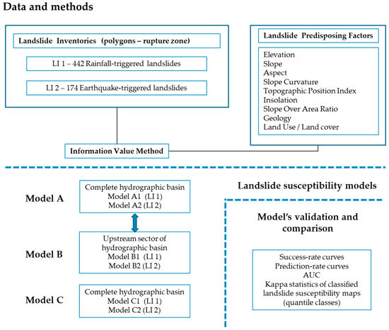
Figure 1.
Data, methods, and modelling strategy.
2.1. Study Area
The study area is the hydrographic basin of Ribeira Grande, which is located on the northern flank of Fogo Volcano, in the central part of the island of São Miguel, Azores (Figure 2).
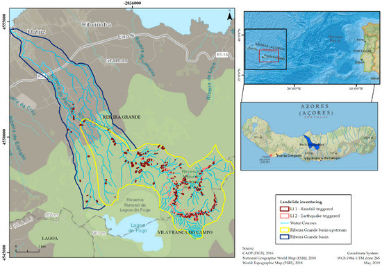
Figure 2.
Location of the study area and landslide inventorying.
The Azores archipelago is located in the North Atlantic Ocean and is composed of nine volcanic islands (Figure 2). From the geodynamic point of view, the archipelago is located in the Triple Azorean Junction [30], where the North American, the African, and the Eurasian lithospheric plates are in contact. Due to its tectonic setting, both volcanic and seismic events occur frequently. The seismicity is intense, with magnitudes up to 7 and variable focal mechanisms indicating dextral and sinistral strike-slip, normal, oblique, and reverse events [31]. The last major seismic event occurred in the Fogo-Congro zone in 2005 and affected the study area.
The study area is part of the Fogo Volcano, a major geomorphological unit covering approximately 150 km2. The Fogo Volcano is a central volcano with maximum elevation of 947 m asl [32]. A caldera containing a permanent lake is located in the central part of the volcano. The hydrographic basin of Ribeira Grande extends along 16.52 km2. The elevation ranges from 0 to 886 m asl. The mean elevation of the basin is 450 m asl and the mean slope is 21°.
In the study area, the lithology is composed by trachytic and basaltic rocks that cover 93.9% and 6.1% of the total area, respectively. These rocks date from the Pleistocene and Holocene [33]. The volcanic materials covering the study area originated from the Fogo Volcano eruptions, whose eruptive products (mostly ash and lapilli) have low values of cohesion and angle of internal friction [32].
The climate setting of the archipelago is influenced by the geographic location of the islands in the middle of the north Atlantic, as well as the local orographic effects. The climate of Azores is a temperate climate (group C) according to Köppen’s classification [34]. However, the spatial distribution of the islands causes the Azores climate to be classified, from East to West, as a transition between the subgroups Cs and Cf, respectively, transitioning from a temperate rainy season with a dry summer to a wet temperate rainy climate in all the seasons. In all cases, the average temperature of the hottest month does not exceed 22 °C [35].
The rainfall regime of Azores is characterized by the occurrence of rainfall episodes throughout the year, even during the summer months, although with much less rain. Rainfall is more abundant in the period from October to December (Figure 3). In Ponta Delgada (São Miguel island), the average annual rainfall is 944 mm, but the yearly rainfall can reach more than 1500 mm in very wet years.
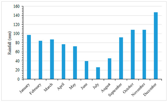
Figure 3.
Average Monthly Rainfall (mm). Meteorological station of Ponta Delgada (normal climatological, 1981–2010. Source: Portuguese Institute of the Sea and Atmosphere, 2017.
2.2. Landslide Inventoring
The study area contains both earthquake-triggered and rainfall-triggered landslides that were inventoried in different moments, using aerial-photo interpretation and extensive field work. The former landslide inventory was made immediately after the earthquakes of September 20 and 21, 2005, using field work and a helicopter mission of the Portuguese Air Force [36]. These seismic events triggered 174 shallow slides in the study area. This event-landslide inventory was given the name “LI 2” along this study area. The latter landslide inventory was made in 2016 and includes 442 shallow slides triggered by rainfall in several periods from 2005 to 2016 [37]. This multi-temporal landslide inventory was given the name “LI 1” in this study area. Both landslide inventories are made of polygons that represent the rupture zone of the shallow slides. As a rule, the accumulation zone of these landslides is not conserved in the landscape as the unstable material was mobilized by debris flows and the fluvial network.
Bearing in mind the second objective of this study, the study area was also considered to model a restricted zone, contained in the hydrographic basin of Ribeira Grande, covering the upstream sector of the basin (9.53 km2). Most of the shallow slides are concentrated in this area (96% of the total landslides inventoried in the study area), comprising 415 slope movements for LI 1 and the complete set of landslides belonging to LI 2.
2.3. Morphometric Attributes of Shallow Slides Triggered by Rainfall and Earthquakes
In this study, 9 morphometric parameters were considered for the characterization of the shallow slides for the comparison between LI 1 and LI 2. The analysis of variance with a factor (one-way analysis of variance (ANOVA)) was used to assess whether the means of two groups of landslides (LI 1 and LI 2) were different [33,38,39]. For each parameter, the mean and standard deviation, the one-way ANOVA F test, and the respective statistical significance level (p-value) area are summarized in Table 1.

Table 1.
One way analysis of variance ANOVA F test and significance level for landslide parameters of inventories of shallow slides for Landslide Inventory 1 (LI 1) and Landslide Inventory 2 (LI 2) (X = average; σ = standard deviation).
When analysing the landslide inventories associated with each triggering factor (LI 1 versus LI 2), some differences were found in relation to their morphometric characteristics. With the exception of parameters associated with the Topographic Position Index, Insolation, and Slope Over Area Ratio, all other parameters attest to the differentiation between considered shallow slide inventories, which is evidenced by the significance levels of Test F being lower than 0.05.
As a rule, the shallow slides belonging to LI 1 (rainfall-triggered) tend to be longer and wider compared to shallow slides included in LI 2 (earthquake-triggered). Figure 4a shows the distribution of the two groups of landslides per area class and confirms the inequality of the landslide inventories. Although shallow slides with a dimension below 100 m2 are dominant in both landslide inventories, their relative importance is much higher in the group of landslides triggered by earthquakes (LI 2 −58% of the total), in comparison to landslides triggered by rainfall (LI 1 −32% of the total). In addition, most landslides belonging to LI 2 (84.1%) have an area less than 200 m2, in contrast to LI 1, where the fraction of landslides below 200 m2 does not exceed 60%.
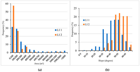
Figure 4.
Distribution of the area (a) and slope (b) per landslides LI 1 and LI 2.
The mean elevation is typically higher in shallow slides belonging to LI 2, which results from their spatial distribution constrained to the upstream sector of the basin. The mean slope is higher in LI 2 shallow slides in comparison with LI 1 shallow slides (53° and 45°, respectively. Figure 4b shows the distribution of the two groups of landslides per slope class and confirms the existing inequality between landslide inventories. The landslides included in LI 1 are mainly concentrated on slopes between 30° and 55° (77% of total), while landslides included in LI 2 mainly occur on slopes between 45° and 65° (84% of total).
2.4. Landslide Susceptibility Modelling
Landslide susceptibility assessment was fulfilled using a data-driven approach—the Information Value (IV) Method [40,41,42,43,44,45,46]).
The information value li of each class within each landslide predisposing factor Xi is given by [40]:
where li is the information value of the variable class Xi; Si is the number of terrain units with shallow slides rupture zone in the presence of the variable class Xi; Ni is the number of terrain units containing the variable Xi; S is the total number of terrain units with shallow slides rupture zones; N is the total number of terrain units.
Negative values of Ii mean that the presence of the variable class is not relevant to shallow slide occurrence. Positive values of Ii indicate a relevant relationship between the presence of the variable class and shallow slide occurrence; the stronger the value, the higher the score [47]. The total information value lj for a terrain unit j is given by [40]:
where lj is the final information value of the terrain unit; n is the number of variables; Xij assumes 0 if the variable class is not present in the terrain unit j or 1 in the opposite case.
The landslide predisposing factors are used as independent variables to assess landslide susceptibility. Their choice was made according to their physical meaning, the availability of data, and by comparison with previous works performed in the São Miguel island [33,48].
In this study, we used 9 landslide predisposing factors (Figure 5) that can be separated into two groups: factors derived from the Digital Elevation Model (DEM) and geoenvironmental factors. The former are the following: Elevation, Slope, Aspect, Slope Curvature, Topographic Position Index (TPI), Insolation, and Slope over Area Ratio. Geoenvironmental factors considered are Geology and Land Use/Land Cover. The landslide predisposing factors were classified following the proposal of Marques [33,49], which was used in a study area similar to the Ribeira Grande basin.
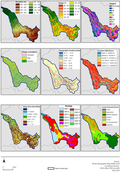
Figure 5.
Predisposing factors used in susceptibility models. Geology classes codes are described in Table 2.
The dependent variable of the models is the shallow slides triggered by rainfall (LI 1) and the shallow slides triggered by earthquakes (LI 2), which were crossed independently with each landslide predisposing factor to weight variable classes.
The entire modelling process was based on grid cells terrain units with 5 × 5 m. The susceptibility maps produced were systematically classified into six quantile classes, preserving an equivalent number of grid cells in each class.
2.5. Validation and Comparison of Landslide Susceptibility Models
The validation of the susceptibility models is essential to evaluate the predictive capacity of the susceptibility maps [9]. The goodness of fit and the predictive capacity for each landslide susceptibility model were evaluated using success rate and prediction rate curves, which express the portion of area required to explain the occurrence of a given percentage of landslides [50]. The success rate curves were computed crossing each landslide susceptibility map with the corresponding landslide inventory used to weight the predisposing factors’ classes. In addition, prediction rate curves were computed by crossing the maps based on rainfall-induced landslides with landslides triggered by earthquakes, and the maps based on landslides triggered by earthquakes with rainfall-induced landslides. The goal of this strategy is to evaluate the capacity of each landslide susceptibility model to predict the location of landslides of the same type associated with a different trigger. In addition, the Area Under Curve (AUC) was computed for both success rate and prediction rate curves, which allows the evaluation of the quantitative performance of each susceptibility model.
The spatial agreement between landslide susceptibility maps was evaluated using Kappa Statistics [51,52]. The Kappa statistic is a measure of similarity between two maps that is based on the percentage of agreement corrected for the fraction of agreement that can result from chance [44,51]. Three Kappa statistics were computed: Kappa location, Kappa histogram, and Kappa index. Kappa location assesses similarity of location concerning the spatial distribution of categories on maps, while Kappa histogram assesses similarity of frequency of categories (landslide susceptibility classes in this study) in both maps. The Kappa index is computed as the product between Kappa location and Kappa histogram [51].
2.6. Modelling Strategy
The modelling strategy is summarized in Figure 1 and encompasses 3 models (A, B, and C), which are subdivided according to the landslide inventory used as the dependent variable (e.g., A1 and A2):
Model A evaluates the landslide susceptibility for the entire hydrographic basin, weighting the class variables of landslide predisposing factors and taking in account the landslide distribution in the complete study area. One model was made for landslides triggered by rainfall (Model A1-LI 1), and another model was made for landslides triggered by earthquakes (Model A2-LI 2).
Model B consists of a reduction of the study area to the upstream sector of the watershed (9.53 km2), where most of the shallow slides are concentrated (see Figure 2). With this procedure we aim to evaluate the effect of the elimination of an extensive area that is not susceptible to landslide occurrence (central and downstream sectors of the basin). Thus, in Model B the class variables of landslide predisposing factors were weighted considering only those landslides located in the upstream sector of the watershed and accounting for the reduction of the study area. As in Model 1, different Models were built for each landslide inventory (Model B1-LI 1, Model B2-LI 2).
Model C consists of applying the scores of variable classes obtained with Model B (B1 and B2) to the entire study area. Again, two Models were built, one for each landslide inventory (Model C1-LI 1, Model C2-LI 2).
3. Results
Results are presented in three sections following the adopted modelling strategy: (i) susceptibility models for the complete hydrographic basin (Model A); (ii) susceptibility models for the upstream sector of the basin (Model B); and (iii) susceptibility models for the complete hydrographic basin using the IV scores of Model B (Model C).
Table 2 shows the IV scores computed for each class of each landslide predisposing factor, obtained for Models A and B, independently for LI 1 and LI 2.

Table 2.
Information Value (IV) scores determined for each class of each predisposing factor. The highest scores are highlighted in bold.
3.1. Model A
The objective of Model A is to verify if the shallow slide inventories associated with different triggering mechanisms (rainfall and earthquake) produce different landslide susceptibility Models for the entire hydrographic basin.
Landslide susceptibility Models A1 and A2 are visually very similar (Figure 6 and Figure 7). Both landslide susceptibility maps show a marked contrast between the downstream and middle sectors of the basin where the classes of low and very low susceptibility predominate, and the upstream sector of the basin, where the classes of high and very high susceptibility are concentrated.
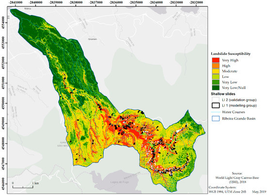
Figure 6.
Model A1: Susceptibility to landslides triggered by rainfall (LI 1) in the entire basin.
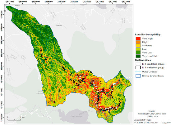
Figure 7.
Model A2: Susceptibility to landslides triggered by earthquake (LI 2) in the entire basin.
This evidence is in consonance with the already mentioned spatial concentration of shallow slides belonging to the two inventories in the upstream sector of the hydrographic basin, where the higher slopes are found. Also, the upper part of the basin is characterized by the presence of trachytic pyroclastic deposits, which are highly susceptible to landslide occurrence. In contrast, the slope angle is typically lower in the downstream and middle sectors of the basin. This fact, together with the occurrence of trachytic domes and flows justify the lower landslide susceptibility.
The slope angle is the most important predisposing factor for both landslide susceptibility Models A1 and A2, although its relevance is higher for Model A2, which is confirmed by the corresponding IV scores for slope angle above 40° that are higher than those for Model A1 (Table 2).
The IV scores of elevation show that slopes from 400 to 500 m asl are more prone to shallow slides induced by rainfall, whereas shallow slides triggered by earthquake are more frequent on slopes from 600 to 700 m asl (Table 2). The SE aspect and concave and convex slope curvature are favourable conditions for the occurrence of shallow slides independently of the trigger (Table 2). Also, the highest scores of slope-over-area ratio are similarly relevant for both landslide susceptibility Models A1 and A2. The Topographic Position Index indicates that landslides induced by rainfall tend to occur near the top and near the bottom of slopes, whereas landslides triggered by earthquakes are more frequent near the bottom of the slope.
Figure 8 summarizes the success rate and prediction rate curves of Models A1 and A2. Therefore, for model A1, the success rate and the prediction rate were obtained by crossing the landslide susceptibility map with LI 1 and LI 2, respectively. The same rationale was applied for the complete set of landslide susceptibility Models.
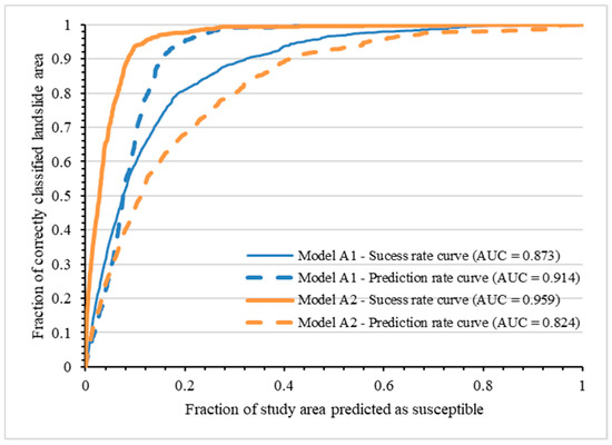
Figure 8.
Success rate and prediction rate curves of landslide susceptibility Models A1 and A2.
Model A1 has a high success rate (AUC = 0.873) and an even better prediction rate (AUC = 0.914). The high success rate is not surprising, since it shows the good fit between the Model and the inventory data that originated it. As for the prediction rate, this is unexpectedly higher than the success rate, indicating that Model A1 is more effective in the independent validation of earthquake-triggered landslides (LI 2) than of rainfall-triggered landslides (LI 1) that were used to construct the Model. On the other hand, Model A2 has a very high success rate (AUC = 0.959) and a considerably lower prediction rate (AUC = 0.824), which was expected, since in the latter case it is an independent validation.
The evaluation of the spatial agreement between Models A1 and A2 was made with Kappa statistics (Table 3). The corresponding landslide susceptibility maps have a kappa index of 0.406, which means that they have a moderate agreement. However, the kappa index increases significantly when only the very high susceptibility class is considered, showing a substantial spatial agreement (0.614).

Table 3.
Kappa values obtained by comparing the susceptibility Model A1 vs. Model A2.
3.2. Model B
Models B1 and B2 (Figure 9 and Figure 10) refine the landslide susceptibility results in the upstream sector of the basin and show a higher spatial variability of susceptibility when compared to the results obtained for the same area with Model A. In addition, it is worth noting the general decrease of IV scores for most landslide predisposing factors, in comparison with Model A, which is evident for models using both landslide inventories (LI 1-Model B1; LI 2-Model B2). Moreover, the spatial distribution of landslide susceptibility is less similar than in Model A, as the very high landslide susceptibility of Model A1 are located in the middle part of the considered study area (Figure 9), where the major rainfall-triggered shallow slides occurred, whereas the high landslide susceptibility of Model A2 are located along two deep carved V-shaped valleys near the upper boundary of the basin (Figure 10), where earthquake-triggered shallow slides are concentrated.
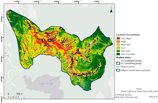
Figure 9.
Model B1: Susceptibility to landslides triggered by rainfall (LI 1) in the upper part of the basin.
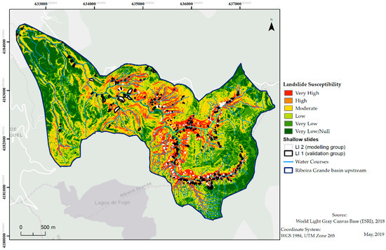
Figure 10.
Model B2: Susceptibility to landslides triggered by earthquakes (LI 2) in the upper part of the basin.
As for Model A, the slope angle is the most important predisposing factor for both landslide susceptibility Models B1 and B2, although the corresponding IV scores of the highest slopes are lower than those of Model A (Table 2), indicating a lower capacity to discriminate between stable and unstable slopes.
The relationship between Models B1 and B2 and elevation is similar to Model A, as shallow slides triggered by earthquakes tend to occur in higher slopes in comparison with shallow slides induced by rainfall (600–700 m asl and 400–500 m asl, respectively).
The aspect S and SE are favourable to landslide triggered by earthquakes, whereas the association between slope aspect and landslides induced by rainfall is not evident (Table 2). Both Models B1 and B2 as positively associated with concave slope curvature, as well as to the highest scores of slopes over area ration (Table 2). The Topographic Position Index indicates that shallow slides tend to occur near the bottom of slopes, independently on the trigger.
The success and prediction rates of Models B1 and B2 (Figure 11), as compared to Model A, decrease consistently. In the case of the Models generated with LI 2 (Models A2 and B2), the Area Under Curve decrease is 0.017 and 0.065 for the success rate and the prediction rate, respectively. In the landslide susceptibility Models produced with LI 1 (Models A1 and B1), the Area Under Curve decrease is even larger, being 0.037 and 0.075 for the success rate and the prediction rate, respectively. It is worth noting that, as observed for Model A, the susceptibility Model built with rainfall-triggered landslides (Model B1) is very effective to predict earthquake-triggered landslides, whereas the inverse is not true (AUC of prediction rates of 0.839 and 0.759, respectively, for Models B1 and B2).
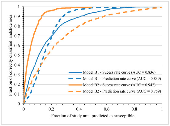
Figure 11.
Success and prediction rate curves of landslide susceptibility Models B1 and B2.
The evaluation of the spatial agreement between Model B1 and B2 shows a kappa index of 0.244, which means that they have a fair agreement. This value tends to increase if only the very low or null susceptibility classes (0.470) and very high susceptibility classes (0.370) are considered, which have a moderate and considerable spatial agreement, respectively (Table 4).

Table 4.
Kappa values obtained by comparing the susceptibility Model B1 vs. Model B2.
3.3. Model C
The IV scores obtained in Model B considering only the upstream section of the basin are more realistic for both landslide inventories (LI 1 and LI 2), as most shallow slides are concentrated in this part of the study area. Thus, in the last modelling step we applied the VI scores of Models B1 and B2 to the entire study area, thus generating two new susceptibility maps, described as Models C1 and C2 (Figure 12 and Figure 13). As expected, the obtained landslide susceptibility maps are similar to the models applied for the entire watershed (Models A1 and A2; Figure 6 and Figure 7). However, the predictive performance of Models C1 and C2 is slightly lower than in Models A1 and A2, as are the success rates (between 0.001 and 0.005) and the prediction rates (between 0.008 and 0.022) (Figure 14).

Figure 12.
Model C1: Susceptibility to landslides triggered by rainfall (LI 1) in the entire basin (using IV scores of Model B1).
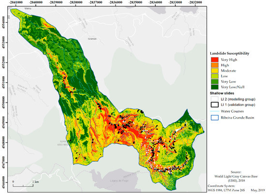
Figure 13.
Model C2: Susceptibility to landslides triggered by earthquakes (LI 2) in the entire basin (using IV scores of Model B2).
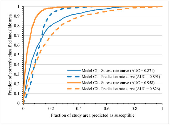
Figure 14.
Success and prediction rate curves of landslide susceptibility Models C1 and C2.
The spatial agreement between landslide susceptibility maps of the entire hydrographic basin, obtained using the IV scores achieved in the upstream sector of the basin (Model C) with their equivalents based on IV scores calculated for the entire basin (Model A), is summarized in Table 5.

Table 5.
Kappa values obtained by comparing the susceptibility Model A vs. Model C.
The concordance between the susceptibility maps associated with landslide belonging to LI 1 (A1 vs. C1) is moderate, which is attested by the kappa index of 0.506. Additionally, agreement is excellent (almost perfect) in the very high and substantial in the high and moderate susceptibility classes (0.636 and 0.637, respectively).
The susceptibility maps associated with landslides belonging to LI 2 (A2 vs. C2) also show a moderate agreement, with a kappa index of 0.492. As in the previous case, the agreement is excellent in the very high susceptibility class, and substantial in the high and moderate susceptibility classes.
4. Discussion
The results obtained with Model A were somewhat unexpected, namely regarding Model A1, which generated a predictive rate curve higher than the success rate curve. In summary, the model produced with the historical inventory of landslides triggered by rainfall (Model 1, LI 1) is very effective in predicting the spatial location of earthquake-triggered landslides (LI 2), which constitute an event-inventory that occurred in 2005. In contrast, the model built with earthquake-triggered landslides (Model 2, LI 2) did not predict well the spatial location of rainfall-triggered landslides (LI 1). These results could be due to the great inequality in the number of inventoried landslides (442 against 174 in LI 1 and LI 2, respectively), and, above all, in the landslide affected area, which is higher in the case of LI 1 by almost one order of magnitude (133,930 m2 versus 18,781 m2 for LI 1 and LI 2, respectively). Previous works have shown the importance of modelling landslide susceptibility independently for each landslide type in the same study area [20,42,53]. Our findings show that these criteria should be also applied when modelling a single landslide type (shallow slides in the study case) if more than one trigger is involved and the landslide inventories are heterogeneous, as is the case here.
The sector considered to produce Model B corresponds to only 57.7% of the total catchment area but contains 93.9% of the landslides of LI 1 and the total set (100%) of landslides of LI 2. Thus, more than 40% of the catchment area, namely the central and downstream sectors, is characterized by conditions very unfavorable to the occurrence of shallow slides. The exercise of modelling the landslide susceptibility by limiting the study area of the upstream sector of the basin showed a decrease of the IV scores of variable classes, indicating a great propensity for landslide occurrence in the generality of landslide predisposing factors, especially the one observed in the higher slope classes. Since most landslides are spatially constrained to the upstream sector, it is considered that the IV scores associated with Model B reflect better the spatial relationship between the independent variables (predisposing factors) and the dependent variable (landslides grouped in LI 1 and LI 2, depending on the respective triggering factor). In fact, the limitation of the study area only to the upper part of the watershed, where most of the landslides are concentrated, determines that the IV scores of the variable classes are not biased by the presence of the middle and downstream parts of the basin, which are not prone to landslide occurrence due to the dominant gentle slopes. Thus, it is demonstrated that the model with better AUC in the success and prediction rates (Model A) may not be the best model of susceptibility, namely in areas with heterogeneous topography and a very unequal spatial distribution of landslides, as it happens in this study area. These results are in agreement with the findings of Steger and Glade [29], who analyzed the susceptibility of landslide occurrence using statistical methods, including trivial areas not prone to landslide activity.
The predictive performance of Models C1 and C2, which were built using IV scores of Model B, is slightly lower than for Models A1 and A2 and should express more rigorously the real capacity of the models to anticipate the spatial location of landslides that will occur in the future in the study area, triggered by rainfall or by earthquakes with location and magnitude equivalent to those recorded in 2005 in the São Miguel island [36].
Figure 15 summarizes the success-rate curves and corresponding AUC of landslide susceptibility models built with LI 1 (rainfall-triggered) (a) and LI 2 (earthquake-triggered) (b).
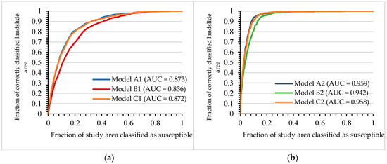
Figure 15.
Success rate curves for landslide susceptibility models built with rainfall-triggered landslides (a) and earthquake-triggered landslides (b).
Model B is based on the scores obtained in the watershed upstream sector and only reports this area. The corresponding success rates (0.846 and 0.941, respectively) are the lowest but are also the more realistic attending to the landslide distribution within the study area.
Model C registers an increase in success rates compared to Model B (0.027 and 0.016. respectively), which can be interpreted as a bias resulting from the enlargement of the study area to a large trivial sector (central and downstream parts of the river basin) with characteristics that are not favourable to slope instability.
Model A results from the IV scores of the variable classes considering the totality of the hydrographic basin and should be compared to Model C. In this comparison, we verified that success rates of Model A are higher than that of Model C (+0.001 and +0.005, respectively). This increase in the success rate is interpreted as a bias associated with the overestimation of the IV scores of the variable classes in Model A, as a result of considering an extensive area not prone to landslide occurrence.
5. Conclusions
The assessment of landslide susceptibility using statistical methods explores the relationships between landslides and predisposing factors based on the contrast between conditions associated with stable and unstable areas. The existence of very sharp contrasts within a study area, caused for example by the presence of extensive areas with reduced or no slope, which are therefore not susceptible to the occurrence of landslides, tends to accentuate the contrast with the areas where landslides are concentrated and to give rise to overly optimistic predictive results.
With this study it was possible to distinguish landslides according to their triggering factor (LI 1 vs. LI 2). Shallow slides triggered by rainfall (LI 1) tend to have a larger dimension compared to those triggered by earthquakes (LI 2). This tendency occurs in the landslide area but also in the length and width of landslides. On the other hand, the landslides of LI 2 occur on steeper slopes and in a higher topographical position, which is understood due to their absolute constraint to the upstream sector of the basin.
It was also demonstrated in this study that when limiting the study area to the upstream sector of the hydrographic basin (Model B), where most of the landslides are concentrated, the models have a lower predictive capacity when compared to the equivalent models that consider the whole hydrographic basin (Model A), which integrates a substantial trivial area where there are no slope instability phenomena. The susceptibility models developed specifically for the watershed upstream sector, although presenting more modest predictive results, reflect in a more realistic way the relationships between the landslides and the predisposing factors and the real capacity to anticipate the spatial location of future landslides.
Regarding Model C, which was elaborated for the entire hydrographic basin based on the IV scores obtained in the upstream sector of the study area, it has a lower performance compared to the models computed for the same area with the IV scores obtained for the entire study area. Nevertheless, Model C (C1 and C2) expresses more accurately the capacity and limitations of the models in anticipating the spatial location of landslides that will occur in the study area in the future. In addition, the modelling performed allowed us to conclude that the model with better AUC in the success and prediction rates may not be the best model of landslide susceptibility. Additional work should be performed in the future in the study area by enlarging the landslide inventories and taking into consideration the influence of rainfall spatial distribution and of earthquake epicenter location on landslide susceptibility.
Author Contributions
C.G., J.L.Z., and R.M. conceptualized the work. R.M. performed the field work in 2005. C.G. performed the field work in 2016 and the landslide susceptibility modelling. C.G., J.L.Z., and R.M. wrote the paper.
Funding
This research was financed by national funds through FCT–Portuguese Foundation for Science and Technology, I.P. (UID/GEO/00295/2019) and was was supported by the project BeSafeSlide—Landslide Early Warning soft technology prototype to improve community resilience and adaptation to environmental change (PTDC/GES-AMB/30052/2017). CG has a PhD Grant supported by the University of Lisbon.
Conflicts of Interest
The authors declare no conflict of interest. The funders had no role in the design of the study; in the collection, analyses, or interpretation of data; in the writing of the manuscript or in the decision to publish the results.
References
- Glade, T.; Crozier, M.J. Landslide Hazard and Risk—Concluding Comment and Perspectives; John Wiley & Sons: Hoboken, NJ, USA, 2012; pp. 765–774. ISBN 9780470012659. [Google Scholar]
- Sestraș, P.; Bilașco, S.; Roșca, S.; Naș, S.; Bondrea, M.; Gâlgău, R.; Vereș, I.; Sălăgean, T.; Spalević, V.; Cîmpeanu, S.; et al. Landslides Susceptibility Assessment Based on GIS Statistical Bivariate Analysis in the Hills Surrounding a Metropolitan Area. Sustainability 2019, 11, 1362. [Google Scholar] [CrossRef]
- Scaioni, M.; Longoni, L.; Melillo, V.; Papini, M. Remote Sensing for Landslide Investigations: An Overview of Recent Achievements and Perspectives. Remote Sens. 2014, 6, 9600–9652. [Google Scholar] [CrossRef]
- Roccati, A.; Faccini, F.; Luino, F.; Ciampalini, A.; Turconi, L.; Roccati, A.; Faccini, F.; Luino, F.; Ciampalini, A.; Turconi, L. Heavy Rainfall Triggering Shallow Landslides: A Susceptibility Assessment by a GIS-Approach in a Ligurian Apennine Catchment (Italy). Water 2019, 11, 605. [Google Scholar] [CrossRef]
- Highland, L.M.; Bobrowsky, P. The Landslide Handbook—A Guide to Understanding Landslides; US Geological Survey: Reston, VA, USA, 2008.
- Guzzetti, F.; Peruccacci, S.; Rossi, M.; Stark, C.P. Rainfall thresholds for the initiation of landslides in central and southern Europe. Meteorol. Atmos. Phys. 2007, 98, 239–267. [Google Scholar] [CrossRef]
- Caine, N. The Rainfall Intensity-Duration Control of Shallow Landslides and Debris Flows. Geogr. Ann. Ser. A Phys. Geogr. 1980, 62, 23–27. [Google Scholar]
- Hungr, O.; Leroueil, S.; Picarelli, L. The Varnes classification of landslide types, an update. Landslides 2014, 11, 167–194. [Google Scholar] [CrossRef]
- Beguería, S. Changes in land cover and shallow landslide activity: A case study in the Spanish Pyrenees. Geomorphology 2006, 74, 196–206. [Google Scholar] [CrossRef]
- Carson, M.A.; Kirkby, M.J. Hillslope Form and Process; Cambridge University Press: Cambridge, UK, 1972. [Google Scholar]
- Iovine, G.G.R.; Greco, R.; Gariano, S.L.; Pellegrino, A.D.; Terranova, O.G. Shallow-landslide susceptibility in the Costa Viola mountain ridge (southern Calabria, Italy) with considerations on the role of causal factors. Nat. Hazards 2014, 73, 111–136. [Google Scholar] [CrossRef]
- Cignetti, M.; Godone, D.; Giordan, D. Shallow landslide susceptibility, Rupinaro catchment, Liguria (northwestern Italy). J. Maps 2019, 15, 333–345. [Google Scholar] [CrossRef]
- Crosta, G.B.; Frattini, P. Distributed modelling of shallow landslides triggered by intense rainfall. Nat. Hazards Earth Syst. Sci. 2003, 3, 81–93. [Google Scholar] [CrossRef]
- Van Asch, T.; Buma, J.; Van Beek, L. A view on some hydrological triggering systems in landslides. Geomorphology 1999, 30, 25–32. [Google Scholar] [CrossRef]
- Roback, K.; Clark, M.K.; West, A.J.; Zekkos, D.; Li, G.; Gallen, S.F.; Chamlagain, D.; Godt, J.W. The size, distribution, and mobility of landslides caused by the 2015 Mw7.8 Gorkha earthquake, Nepal. Geomorphology 2018, 301, 121–138. [Google Scholar] [CrossRef]
- Strupler, M.; Danciu, L.; Hilbe, M.; Kremer, K.; Anselmetti, F.S.; Strasser, M.; Wiemer, S. A subaqueous hazard map for earthquake-triggered landslides in Lake Zurich, Switzerland. Nat. Hazards 2018, 90, 51–78. [Google Scholar] [CrossRef]
- Hadi, A.I.; Brotopuspito, K.S.; Pramumijoyo, S.; Hardiyatmo, H.C. Regional Landslide Potential Mapping in Earthquake-Prone Areas of Kepahiang Regency, Bengkulu Province, Indonesia. Geosciences 2018, 8, 219. [Google Scholar] [CrossRef]
- Villeneuve, M.; Dellow, S.; Massey, C.I.; Mccoll, S.T.; Townsend, D.B. Landslides caused by the 14 November 2016 Kaikoura earthquake, South Island. In Proceedings of the 20th Symposium of the New Zealand Geotechnical Society, Napier, New Zealand, 24 November 2017; pp. 1–8. [Google Scholar]
- Sidle, R.C.; Ochiai, H. Landslides: Processes, Prediction, and Land Use; Springer: Berlin/Heidelberg, Germany, 2006; Volume 18. [Google Scholar]
- Heerdegen, R.G. Landslides: Causes, Consequences and Environment; Croom Helm: Kent, UK, 1989; Volume 45, pp. 93–94. [Google Scholar]
- Keefer, D.K. Landslides caused by earthquakes. Geol. Soc. Am. Bull. 1984, 95, 406–491. [Google Scholar] [CrossRef]
- Lin, G.-W.; Chen, H.; Chen, Y.-H.; Horng, M.-J. Influence of typhoons and earthquakes on rainfall-induced landslides and suspended sediments discharge. Eng. Geol. 2008, 97, 32–41. [Google Scholar] [CrossRef]
- Lin, C.-W.; Liu, S.-H.; Lee, S.-Y.; Liu, C.-C. Impacts of the Chi-Chi earthquake on subsequent rainfall-induced landslides in central Taiwan. Eng. Geol. 2006, 86, 87–101. [Google Scholar] [CrossRef]
- Yamagishi, H.; Iwahashi, J. Comparison between the two triggered landslides in Mid-Niigata, Japan by July 13 heavy rainfall and October 23 intensive earthquakes in 2004. Landslides 2007, 4, 389–397. [Google Scholar] [CrossRef]
- Zhang, S.; Zhang, L.; Glade, T. Characteristics of earthquake- and rain-induced landslides near the epicenter of Wenchuan earthquake. Eng. Geol. 2014, 175, 58–73. [Google Scholar] [CrossRef]
- Zêzere, J.L.; Henriques, C.S.; Garcia, R.A.C.; Oliveira, S.C.; Piedade, A.; Neves, M. Effects of landslide inventories uncertainty on landslide susceptibility modelling. In Landslide Processes: From Geomorphologic Mapping to Dynamic Modelling; Mallet, J.-P., Remaitre, A., Boggard, T., Eds.; CERG Editions: Strasbourg, France, 2009; pp. 81–86. [Google Scholar]
- Bai, S.-B.; Wang, J.; Lü, G.-N.; Zhou, P.-G.; Hou, S.-S.; Xu, S.-N. GIS-based logistic regression for landslide susceptibility mapping of the Zhongxian segment in the Three Gorges area, China. Geomorphology 2010, 115, 23–31. [Google Scholar] [CrossRef]
- Li, Y.; Chen, G.; Tang, C.; Zhou, G.; Zheng, L. Rainfall and earthquake-induced landslide susceptibility assessment using GIS and Artificial Neural Network. Nat. Hazards Earth Syst. Sci. 2012, 12, 2719–2729. [Google Scholar] [CrossRef]
- Steger, S.; Glade, T. The Challenge of “Trivial Areas“ in Statistical Landslide Susceptibility Modelling. In Proceedings of the Workshop on World Landslide Forum: Advancing Culture of Living with Landslides, Ljubljana, Slovenia, 29 May–2 June 2017. [Google Scholar]
- Laughton, A.S.; Whitmarsh, R.B. The Azores-Gibraltar Plate Boundary. In NATO Advanced Study Institute, Proceedings of the Geodynamics of Iceland and the North Atlantic; Springer: Berlin/Heidelberg, Germany, 1974. [Google Scholar]
- Madeira, J.; Brum da Silveira, A.; Hipólito, A.; Carmo, R. Active tectonics along the Eurasia-Nubia boundary: Data from the central and eastern Azores Islands. In Geological Society Memoir No. 44; Geological Society of America: Boulder, CO, USA, 2015; Volume 44, pp. 15–32. [Google Scholar]
- Wallenstein, N. Estudo da história eruptiva recente e do comportamento eruptivo do vulcão Fogo (S.Miguel, Açores). Avaliação preliminar do hazard. Ph.D. Thesis, Universidade dos Açores, Ponta Delgada, Portugal, 1999. [Google Scholar]
- Marques, R.T.F. Estudo de movimentos de vertente no concelho da Povoação (ilha de São Miguel, Açores): Inventariação, caracterização e análise da susceptibilidade. Ph.D. Thesis, Geological Risks, University of Azores, Ponta Delgada, Portugal, 2013. [Google Scholar]
- Chazarra, A.; Baceló, A.M.; Pires, V.; Cunha, S.; Silva, A.; Marques, J.; Carvalho, F.; Mendes, M.; Neto, J.; Mendes, L. Climate Atlas of the Archipelagos of the Canary Islands, Madeira and the Azores; Department of the State Meteorological Agency of Spain and Department of Meteorology and Climatology of the Institute of Meteorology: Lisbon, Portugal, 2011. [Google Scholar]
- Azevedo, E. Condicionantes dinâmicas do clima do Arquipélago dos Açores. Elementos para o seu estudo. Açoreana 2001, 9, 309–317. [Google Scholar]
- Marques, R.; Queiroz, G.; Coutinho, R.; Zêzere, J. Actividade geomorfológica desencadeada pela crise sísmica de 2005 no Vulcão do Fogo (S. Miguel, Açores): Avaliação da susceptibilidade com recurso a regressão logística. In Proceedings of the Publicações da Associação Portuguesa de Geomorfólogos, Funchal, Portugal, 12–14 October 2006; pp. 47–61. [Google Scholar]
- Gordo, C. Modelação da Suscetibilidade à Rutura de Movimentos de Vertente: Ilha de São Miguel, Açores. Master’s Thesis, Master’s Degree in Geographical Information Systems and Modelling applied to Spatial Planning, Institute of Geography and Spatial Planning, Lisbon, Portugal, November 2017. [Google Scholar]
- Keefer, D.K. Statistical analysis of an earthquake-induced landslide distribution—The 1989 Loma Prieta, California event. Eng. Geol. 2000, 58, 231–249. [Google Scholar] [CrossRef]
- Jacobs, L.; Dewitte, O.; Poesen, J.; Sekajugo, J.; Nobile, A.; Rossi, M.; Thiery, W.; Kervyn, M. Field-based landslide susceptibility assessment in a data-scarce environment: The populated areas of the Rwenzori Mountains. Nat. Hazards Earth Syst. Sci. 2018, 18, 105–124. [Google Scholar] [CrossRef]
- Yin, K.L.; Yan, T.Z. Statistical Prediction models for slope instability of metamorphosed rocks. In Proceedings of the 5th International Symposium on Landslides, Lausanne, Switzerland, 10–15 July 1988; Volume 2, pp. 1269–1272. [Google Scholar]
- Corominas, J.; van Westen, C.; Frattini, P.; Cascini, L.; Malet, J.-P.; Fotopoulou, S.; Catani, F.; Van Den Eeckhaut, M.; Mavrouli, O.; Agliardi, F.; et al. Recommendations for the quantitative analysis of landslide risk. Bull. Eng. Geol. Environ. 2014, 73, 209–263. [Google Scholar] [CrossRef]
- Zêzere, J.L. Landslide susceptibility assessment considering landslide typology. A case study in the area north of Lisbon (Portugal). Nat. Hazards Earth Syst. Sci. 2002, 2, 73–82. [Google Scholar] [CrossRef]
- Nandi, A.; Shakoor, A. A GIS-based landslide susceptibility evaluation using bivariate and multivariate statistical analyses. Eng. Geol. 2010, 110, 11–20. [Google Scholar] [CrossRef]
- Zêzere, J.; Pereira, S.; Melo, R.; Oliveira, S.; Garcia, R.A.C. Mapping landslide susceptibility using data-driven methods. Sci. Total Environ. 2017, 589, 250–267. [Google Scholar] [CrossRef]
- Conforti, M.; Robustelli, G.; Muto, F.; Critelli, S. Application and validation of bivariate GIS-based landslide susceptibility assessment for the Vitravo river catchment (Calabria, south Italy). Nat. Hazards 2012, 61, 127–141. [Google Scholar] [CrossRef]
- Guillard, C.; Zêzere, J.; Guillard-Gonçalves, C. Landslide Susceptibility Assessment and Validation in the Framework of Municipal Planning in Portugal: The Case of Loures Municipality. Environ. Manag. 2012, 50, 721–735. [Google Scholar] [CrossRef]
- Yan, T.Z. Recent advances of quantitative prognoses of landslides in China. In Proceedings of the Fifth International Symposium on Landslides, Lausanne, Switzerland, 10–15 July 1988; pp. 1263–1268. [Google Scholar]
- Marques, R.; Amaral, P.; Zêzere, J.; Queiroz, G.; Goulart, C. Estudo comparativo de diferentes métodos probabilísticos para a avaliação da susceptibilidade à ocorrência de movimentos de vertente: Um caso de estudo no vale da Ribeira Quente (S. Miguel, Açores). In Proceedings of the Publicações da Associação Portuguesa de Geomorfologia, Braga, Portugal, 16–18 October 2008; pp. 183–190. [Google Scholar]
- Marques, R.; Amaral, P.; Araújo, I.; Gaspar, J.L.; Zêzere, J.L. Chapter 13 Landslides on São Miguel Island (Azores): Susceptibility analysis and validation of rupture zones using a bivariate GIS-based statistical approach. In Geological Society Memoir No. 44; Gaspar, J.L., Guest, J.E., Duncan, A.M., Barriga, F.J.A.S., Chester, D.K., Eds.; Geological Society: London, UK, 2015; Volume 44, pp. 167–184. [Google Scholar]
- Santacana, N.; Corominas, J. Validation de mapas de susceptibilidad a los deslizamientos superficiales. Influencia de la heterogenidad geológica. In Proceedings of the V Simposio Nacional sobre Taludes y Laderas Inestables, Volume II, Madrid, Spain, 27–30 November 2001; Sopeña, J., Rodrígues, L., Vilches, J.M., Oteo, I., Soriano, C., Alonso, A., Corominas, E., Eds.; pp. 475–485. [Google Scholar]
- Visser, H.; De Nijs, T. The Map Comparison Kit. Environ. Model. Softw. 2006, 21, 346–358. [Google Scholar] [CrossRef]
- Cohen, J. A Coefficient of Agreement for Nominal Scales. Educ. Psychol. Meas. 1960, 20, 37–46. [Google Scholar] [CrossRef]
- Cruden, D.M.; Varnes, D.J. Landslides: Investigation and Mitigation. Chapter 3—Landslides Types and Processes; Transportation Research Board: Washington, DC, USA, 1996. [Google Scholar]
© 2019 by the authors. Licensee MDPI, Basel, Switzerland. This article is an open access article distributed under the terms and conditions of the Creative Commons Attribution (CC BY) license (http://creativecommons.org/licenses/by/4.0/).