1. Introduction
A large part of the world’s coastline is threatened by human and environmental changes, such as urbanization, sea level rise, and possible increase in storm activity [
1,
2]. Despite global concerns about these issues, human activity along coastlines has been intensifying worldwide with associated important changes for the coastline [
3,
4,
5]. Tidal dynamics strongly impact the fate and transport of sediments, contaminants, and the morphological evolution of these environments, which prompts the continuous attention to the complex interaction between tidal motion, and sedimentary processes. Furthermore, while tide dominance is often associated with meso- or macro-tidal conditions, it can also interest locations with a small tidal range given the limited wave action, and a large tidal prism [
2,
6,
7,
8].
Along coastal environments, the tides interact with the variable bathymetry leading to the creation of complex residual flow and residual sediment transport due to varying topography, bottom friction, and tidal asymmetries. Residual currents and net transport result thus from non-linear processes and their values can be calculated as an average over multiple tidal cycles [
9,
10,
11,
12]. The idea of a morphodynamic equilibrium is a widely investigated concept referring to the mutual adjustment of topography and fluid-dynamics until conditions of zero net sediment accumulation and/or erosion are reached [
13,
14]. The time scale related to the morphological equilibrium is generally considered long compared to the morphological response time [
15]. Many studies have focussed on the idea of morphodynamic equilibrium, including small scale systems, which are typically categorized as a wave, river, or tidally-dominated, up to the spatial scale of estuaries and tidal inlets [
14,
16]. However, there is a paucity of studies exploring the idea of morphodynamic equilibrium at a larger regional scale [
17].
On the basis of conservation of mass, and depending on the balance of sediment flux divergence, a static equilibrium is present when there is no transport, while a dynamic equilibrium is present when the sediment flux divergence is balanced by source/sink terms, which can be either constant or time-dependent; for the latter, even if the bed might accommodate locally to the changing conditions, there is no net change when considering the system in the long-term. In the case of estuaries, Van der Wegen and Roelvink [
18], distinguished two major morphological timescales connected to the morphodynamic evolution of estuaries i.e., a decadal time scale linked to the evolution of channel-shoal patterns, and a time scale ranging from centuries to millennia connected to the evolution of the longitudinal bed profile. For the latter, they identified tidal asymmetry in terms of differences between ebb and flood velocities as the main driver.
The impact of the sea level rise (SLR) on the morphological evolution of tidal environments has been investigated by Stefanon et al. [
19], who suggests a rapid adaptation of tidal network pattern to changes in tidal prisms. Ganju and Schoellhamer [
20], and Dissanayake et al. [
21] assessed the morphodynamic impact of SLR on inlet systems using numerical models; both concluded that intertidal areas would drown under realistic SLR scenarios, and Dissanayake et al. [
21] concluded that SLR enhances flood dominance. The results from Van der Wegen [
22] demonstrate that the morphological scale of adaptation to environmental factors can be long, so that, while the system might currently appear in equilibrium, further development could happen at a longer time scale. Van der Wegen [
22] investigated the impact of SLR on an idealized channel geometry; numerical experiments showed that under realistic SLR scenarios, intertidal areas tend to disappear, and the basin shifts from being an exporting system towards an importing system. Specifically, they found that the presence of SLR disturbs the tidal propagation balance, causing an increased distortion, and over-tides generation. The study by Van der Wegen and Roelvink [
18] showed that river discharge and density currents do not significantly affect the long term morphology, suggesting that the morphological evolution of tidal systems is mainly dictated by the major tidal forcing, and sediment fractions availability at the bottom; the latter considerations are based on decadal scale morphological updates registered in the Western Scheldt estuary.
The results from [
23,
24,
25] suggest that, in tidally dominated systems, the morphological evolution of the bottom asymptotically tends toward a dynamic equilibrium configuration, characterized by relatively small net sediment fluxes. The authors investigated the existence of a long term equilibrium or quasi-equilibrium, for tide-dominated channels and well-mixed estuaries, by accounting for the morphological updates at the bottom. They found that, given the tidal input at the mouth of the tidal channel, at a century time-scale, the longitudinal profile evolves from an arbitrary initial condition to a final equilibrium configuration characterized by a shallow area in the landward portion of the channel, whose concavity increases with channel convergence, and such that the relationship between the tidal prism and cross-sectional area evolves from an arbitrary distribution to a Jarret’s type law. Furthermore, their results suggest that the evolution of the bed tends to reduce the initial sediment transport asymmetry, leading to a vanishing net sediment flux in the channel where transport patterns become more symmetrical [
23,
24,
26].
While the hypothesis of dynamic equilibrium condition for tidally dominated systems was initially explored for single funnel-shaped channels, successive work has been done suggesting that the idea of tidal equilibrium can be extended to whole systems, such as the Ganges Delta, Bangladesh [
17], and Fly river delta, Papua New Guinea [
27], as well as to the conditions where riverine flow is also present [
28].
Despite the increasingly large body of knowledge and insightful studies on the South-East of England [
29,
30,
31,
32,
33], little information is available on the detailed tidally induced sediment transport, and morphological evolution of the system.
Embedded within the southeast part of the North Sea, the large-scale residual circulation of the area has been studied for a long time: The southern portion of the Suffolk and Essex coastline presents northwest directed surface currents coming from the English Channel, while the northern portion of the study area is partially affected by the large anticlockwise gyre generated by the mixing water of the North Atlantic [
34,
35]. The majority of the existing field and numerical studies, conducted in the study area, are based on relatively large-scale and coarse resolution models. These models were developed at the scale of the North Sea, rather than at a coastline scale, and have sometimes neglected tidally-induced morphological changes, as well as the availability and resuspension of bottom sediments [
36] which are instead accounted for in this study.
The aim of this theoretical work is to better understand the regional-scale sediment transport processes, and their changes as a consequence of long term (century scale) tidally-induced morphological variations and sea level changes. The tendencies of the system are assessed by considering the morphological evolution of the system for different sea level rise scenarios, and by analyzing the spatial distribution of the net transport and residual currents, before and after a century scale morphological evolution and for different sea level variations. The morphological evolution of the system, as well as the hydrodynamics, and sediment transport processes have been simulated using the numerical model Delft3D. The results about the following are presented: (i) Simulated long-term morphological changes in the area; (ii) changes in net transport as a consequence of tidally-induced morphological changes; (iii) and changes in the hydrodynamic and sediment transport as a consequence of sea level variations. The outcomes from this modelling work contribute to the ongoing discussion about coastal morphodynamic and coastal change under sea level variations. For the study area, the findings represent a first-step for a better understanding of the changes in sediment transport dynamics under morphological variations, and allow the impact of tides to be isolated from one of the other external agents. In general, the results might also help unravel the complex dynamics regulating the long-term evolution of tidally-dominated systems.
2. Study Site
The coastline of South East England is a region of enormous ecological and economic importance, and is also unique from an environmental standpoint, given the natural variety of its shoreline, which includes a mosaic of salt marshes, soft cliffs, and sand dunes [
37,
38,
39,
40,
41,
42].
Tides in the North Sea are mainly semi-diurnal, and progress anticlockwise, with the largest amplitudes occurring in the eastern England and German Bight coasts [
43]. Across the South East English coast, the tide is meso- to macro-tidal and tidal range and tidal phase vary significantly, due to the vicinity to the North-Sea amphidromic system. Given the complexity of the various processes at play, there are large uncertainties (±50%) about the sediment budget in the area [
30,
44]. For the North Sea as a whole, sediment supplies include transport from the North Atlantic Ocean and the English Channel (quantified as 10 × 10
6 ta
−1), and those being eroded from the seafloor (6–7.5 × 10
6 ta
−1) and the Norfolk cliffs (6.65 × 10
5 ta
−1); fluvial sediment supplies are instead considered negligible [
44]. Finally, several turbidity studies have identified offshore locations around the Norfolk banks with a high sediment concentration, i.e., the East Anglian plume which is more pronounced in winter [
30].
The South East England coastline is characterized by a variety of shorelines, from sandy beaches, to saltmarshes, shingle banks and soft cliffs (cf. [
37]). The coastline itself is a submerged low coastline, and geologically the area is one of the non-resistant Quaternary strata. The northern portion of the coastline, around Hunstanton, is characterized by soft glacigenic cliffs composed of mainly chalk. Due to its gradual eastward dip, the chalk goes below the sea level near Sheringham, where it is succeeded by Tertiary deposits. Glacial beds cover the Cretaceous chalk and Tertiary deposits. North Norfolk is characterized by both back-barrier and open coast saltmarshes [
45,
46]. The marshland comes to an end at Weybourn, and from there until the Thurne River (around 52.7 N 1.67 E), the area is characterized by soft cliffs of varying heights. Erosive cliffs continue south and give rise to a relatively smooth shoreline profile. Marsh areas and vegetated surfaces can be especially relevant for the mitigation of extreme water levels [
46,
47,
48,
49]. Five major nesses, i.e., projections originating from sandy deposits, are then present along the coast at Winterton (around 52.72N, 1.7E), Caister (52.62N, 1.74E), Lowestoft (52.48N, 1.76E), Benacre (52.38N, 1.71E) and Thorpeness (52.17N, 1.61E) [
50]. Sub-tidal sandbank features are also common. The Norfolk coastline is characterized by headland-associated banks in the form of alternating ridges, with recessional headlands; the Suffolk coastline is characterized by banner banks related to non-recessional banks; the mouth of the Thames comprises wide mouth ridges, and the area immediately south of the Thames is characterized by both alternating ridges with recessional headlands, and banner banks [
31]. South of the Thames, several other shoreline features alternate; for instance, the area around the Thanet and Dover districts, is made of pocket beaches or sandstone cliffs. In between the Folkestone and Lydd ranges there is a relatively wide sandy beach, while the most south portion around Beachy Head presents a chalk headland formed in the late Cretaceous.
3. Methods
Herein we use the computational fluid dynamics package Delft3D [
51], which allows the simulation of hydrodynamic, sediment transport, and morphological processes. Delft3D-FLOW is the hydrodynamic module of the package, and solves the unsteady shallow water equations, following the Boussinesq approximation [
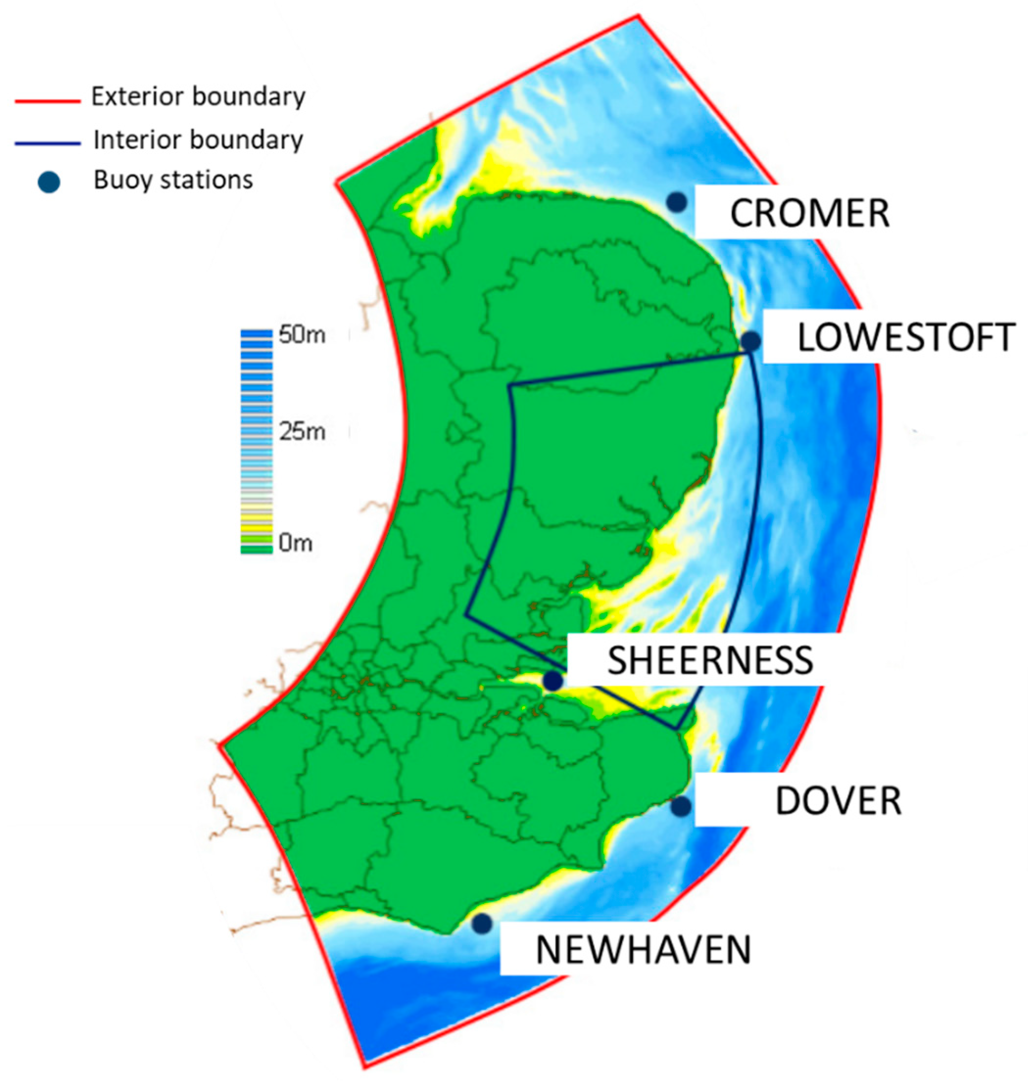
51]. The model is divided into two separate domains (
Figure 1), which are fully coupled, and exchange information along internal boundaries (blue lines) through the domain decomposition option. The domain decomposition option allowed a higher resolution for the domain to be obtained within the internal boundaries. The average grid size for the exterior domain is 1500 × 500 m, and for the smaller domain is 400 × 200 m. Sediment transport and morphology modules support both bedload and a suspended load of non-cohesive sediments, and suspended load of cohesive sediments.
For the cohesive sediment fractions, the Partheniades-Krone formulation [
52] is used to calculate the exchange of fluxes between the water phase and the bed. For non-cohesive fractions, sediment fluxes and settling velocity are calculated following the van Rijn approach [
53], and the transfer of sediments between the bed and the water column is modelled using source and sink terms that exchange sediments through a reference layer, located above the Van Rijn reference height [
53,
54]. More information about the model can be found in DELFT Hydraulics, 2014 [
55].
Bathymetry data are based on 30 × 30 m tiles of the Arcsecond Gridded Bathymetry (ASC geospatial data) product, retrieved from the EDINA Marine Digimap download service (
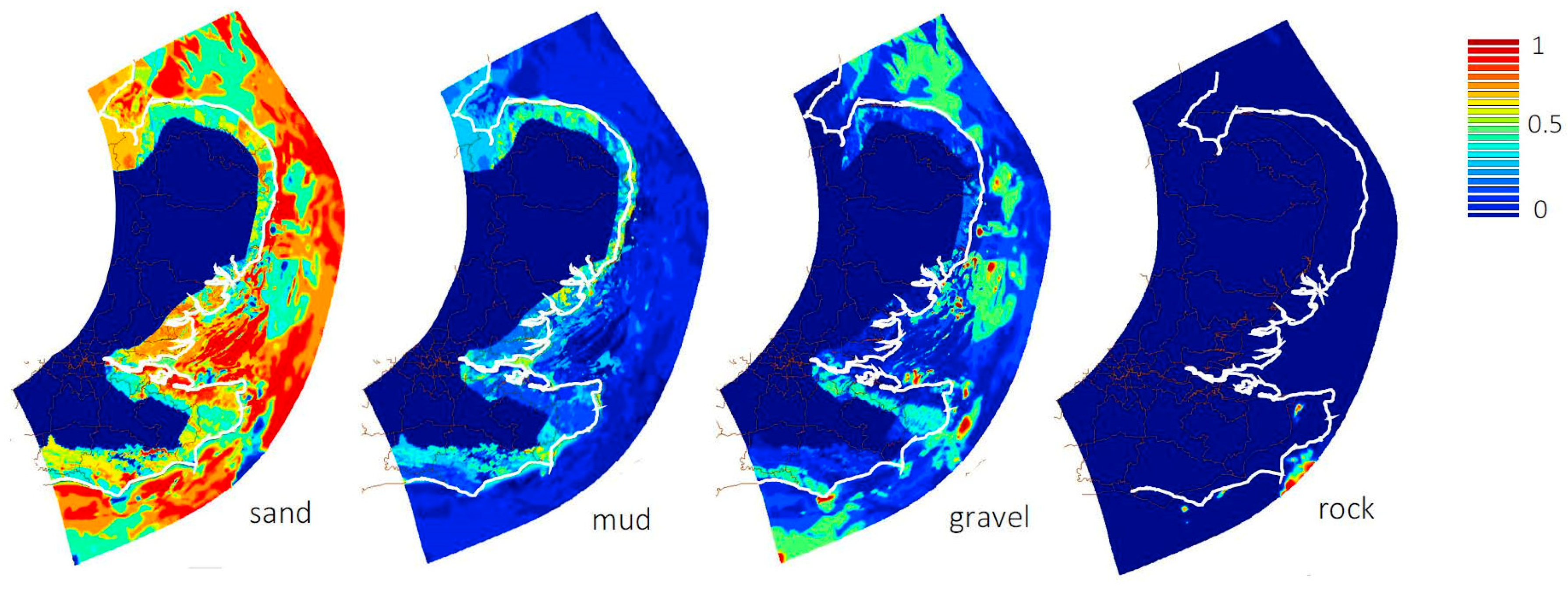
http://digimap.edina.ac.uk/). For the interior part of the shoreline, Digital Terrain Model (DTM) data from LiDAR surveys at 2 m resolution were used, which were downloaded from the UK Environment Agency’s LiDAR data archive. Spatially varying Vertical Offshore Reference Frame (VORF) corrections, provided by the UK Hydrographic Office, were applied to account for the fact that bathymetric data were referred to the Lowest Astronomical Tide, and LiDAR data were referred to Ordnance Datum. VORF corrections were thus used to refer both datasets to the mean sea level. The input for the initial spatial distribution of sediments at the bottom was created based on data derived from the British Geological Survey (BGS), GIS-maps for seabed sediments, and parent material for the more landward side of the domain. Bottom sediments are divided into four main sediment classes, i.e. sand, gravel, mud, and rock (
Figure A1).
When taking the morphological evolution into account a morphological scale factor,
n, of 100 is considered. This factor increases the incremental depth changes at each time step by a constant
n, so that morphological changes over one simulated tidal cycle are representative of those over
n cycles; this is similar to the concept of an elongated tide proposed by Latteux [
56]. From a numerical modelling point of view, one of the key issues of long term simulations is finding ways to tie together short term hydrodynamic processes varying over an hourly time scale, and longer term morphological changes taking place at a yearly time scale, and which are, therefore, computationally expensive to model without morphological accelerator factors. Classical techniques to overcome this problem include tide-averaging methods, continuity corrections, rapid assessment of morphology methods, and the online approach with morphological factor. The latter is currently one of the most commonly used, and constitutes the technique adopted in this study. The application of a morphological factor has been found to significantly improve results with respect to the other techniques, and in the case of highly dynamic coastlines [
57]. Lesser [
58] tested the impact of different morphological factors on numerical simulation outcomes, and found that, morphological scale factors ranging from 1 to 100 lead to very similar morphological results with only minimum discrepancies. Van der Wegen and Roelvink [
18] showed that for long term simulations of tidally dominated systems, the morphological characteristics of the system are maintained for morphological factors up to 400. Under river-dominated conditions, Edmonds and Slingerland [
59] conducted a series of sensitivity analysis within the context of river deltas to test the dependency of results on the morphological factor, and found that, up to a morphological factor of 200, the numerical technique did not impact the morphodynamic evolution. For this study, the use of a morphological factor of 100 is therefore adequate.
The exterior boundary conditions are provided by the Extended Area Continental Shelf Model fine grid (CS3X) having 1/9° latitude by 1/6° longitude (approximately 12 km) resolution, and covering areas from 40°07′ N to 62°53′ N, and from 19°50′ W to 12°50′ E. The exterior boundary is evenly divided into 72 segments (each segment covers about 10 cells) which receive spatially varying inputs from CS3X. Simulations are run from June 2008 to July 2009.
The model was calibrated in Leonardi and Plater [
60]. Model accuracy was evaluated using the Brier Skill Score method [
61]. The skill class was assumed to be excellent for score values in between 0.65–1, very good for 0.65–0.5, good for 0.5–0.2, and poor for less than 0.2 [
62,
63,
64,
65]. The model predicted water levels were compared against measurements taken at 5 buoy stations distributed along the coast (
Figure 1). Scores are excellent with values ranging from 0.84 to 0.97, and modelled tidal levels show good agreement with the instrumental data. We refer to Leonardi and Plater [
60] for more information on model setup and validation.
Apart from the one year simulation, including the morphological evolution of the system, additional simulations were also run with the same hydrodynamic forcing, but two different bathymetries, which were fixed in time and represented the current, and the 100-year evolved morphology. An additional numerical experiment was also run to test the influence of a gradual and linear increase in sea level of 1 cm/year. This very high sea level rise value falls under the 2100 sea level rise projection for the RCP8.5 scenario, and was chosen to highlight the trends caused by a gradual increase in water levels. Finally, to investigate the impact of the sole water level changes, a set of simulations with increased sea level values and a constant morphology were also run.
4. Results
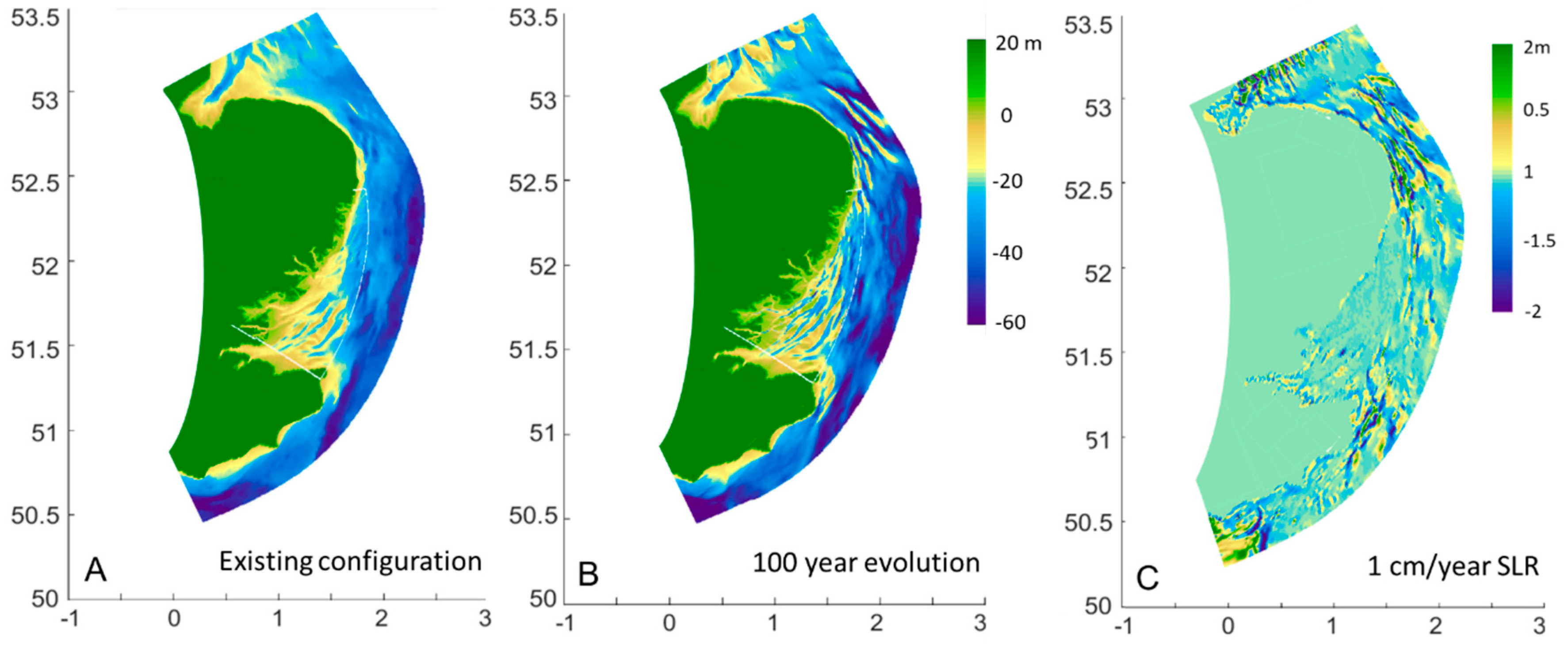
Model results in relation to the morphological evolution of the system at a century time scale (
Figure 2a, b) indicate a steepening of existing sand banks, especially within the Thames estuary, and in the Northeastern portion of the domain, where banks become higher and new ones tend to form. The central part of the domain, covered by the higher resolution grid, is characterized by a marked steepening of the mouth ridges, which become more defined, with higher central islands and deeper surrounding channels. New small ridges also start to form around and above 52 degree latitude. In the northeast, the coastlines adjacent to the accreting sand banks tend to erode, while no significant sediment removal from the coastline areas can be noticed for the southernmost portion of the domain. Morphological results have been obtained by running the numerical simulation for one year, with a morphological factor of 100, and might be thus considered representative of the tidally-induced morphological evolution of the system at a century time scale, and under a simplified scenario including the sole tidal influence. The enhancement of sandbank features can be explained by considering the existence of recirculating gyres which typically establish around banks, due to frictional torques, and cause the potential accumulation of sand on the top of the banks [
10,
32,
66].
When a constant increase in sea level is taken into account (
Figure 2C), the morphological evolution of the system follows a similar but enhanced trend, which results in higher sand bank features, and deeper erosional trends in the northern part of the coastline at around 52.7 degree latitude. Maximum differences in elevation between the non-sea level rise scenario, and the sea level rise test-case, are up to 2 m (
Figure 2C).
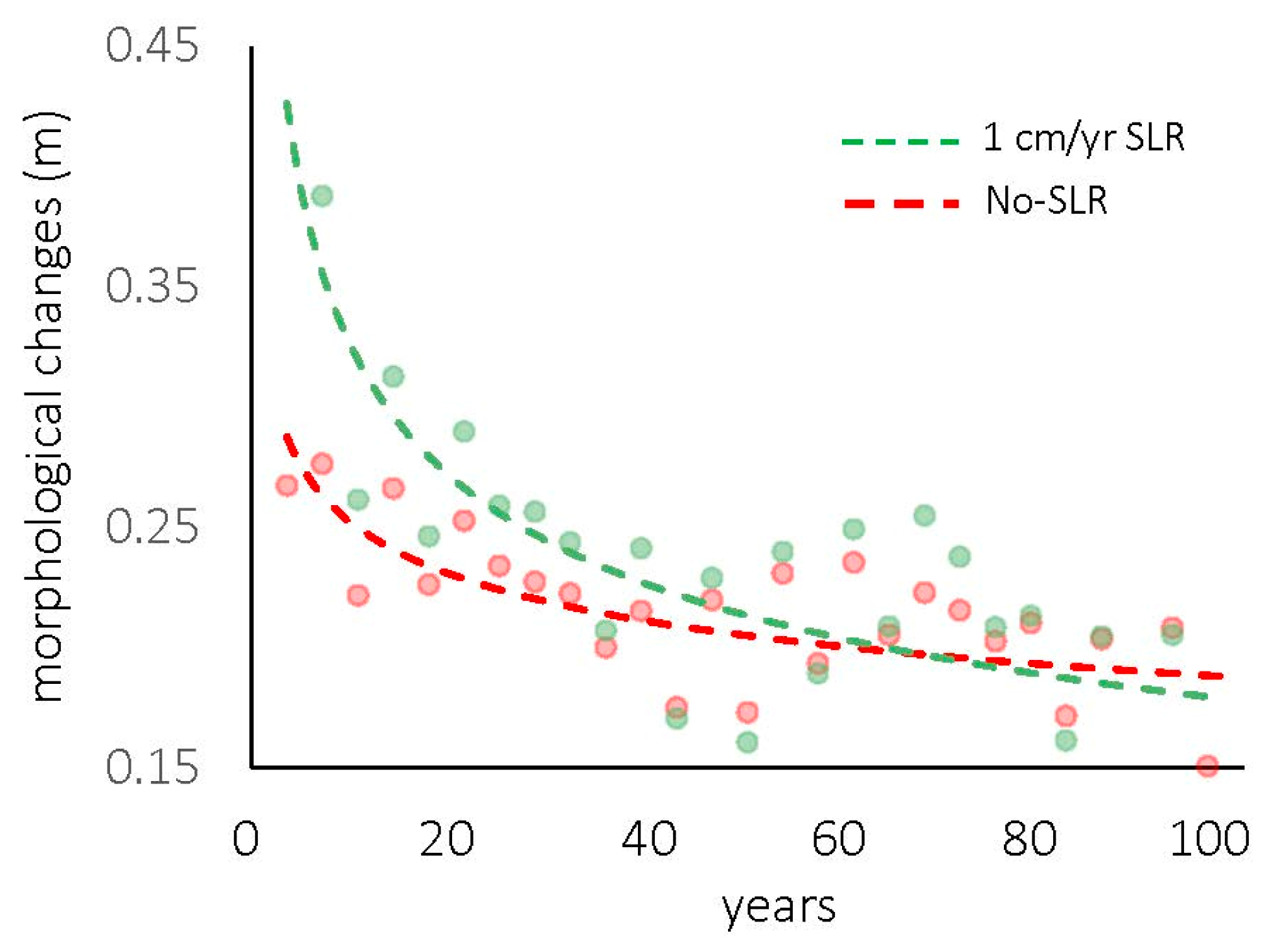
Figure 3 shows variations in bed level as a function of time, for the morphological simulations presented above. The values presented in the figure have been averaged across the entire domain, and hence account for regions having different topographic and bed composition features. The changes in bed level tend to decrease in time, and the morphological evolution by the end of the 100 year period is significantly slower than that at the beginning of the simulated period. By the end of the 100-year period, morphological changes for all test cases attain similar plateau values which are closer to zero. However, the test case with a constant rate of sea level rise show significantly more pronounced morphological changes at the beginning of the study period, suggesting a larger sediment flux divergence and/or convergence patterns at the start, and a sharper decline of the morphological variations in time.
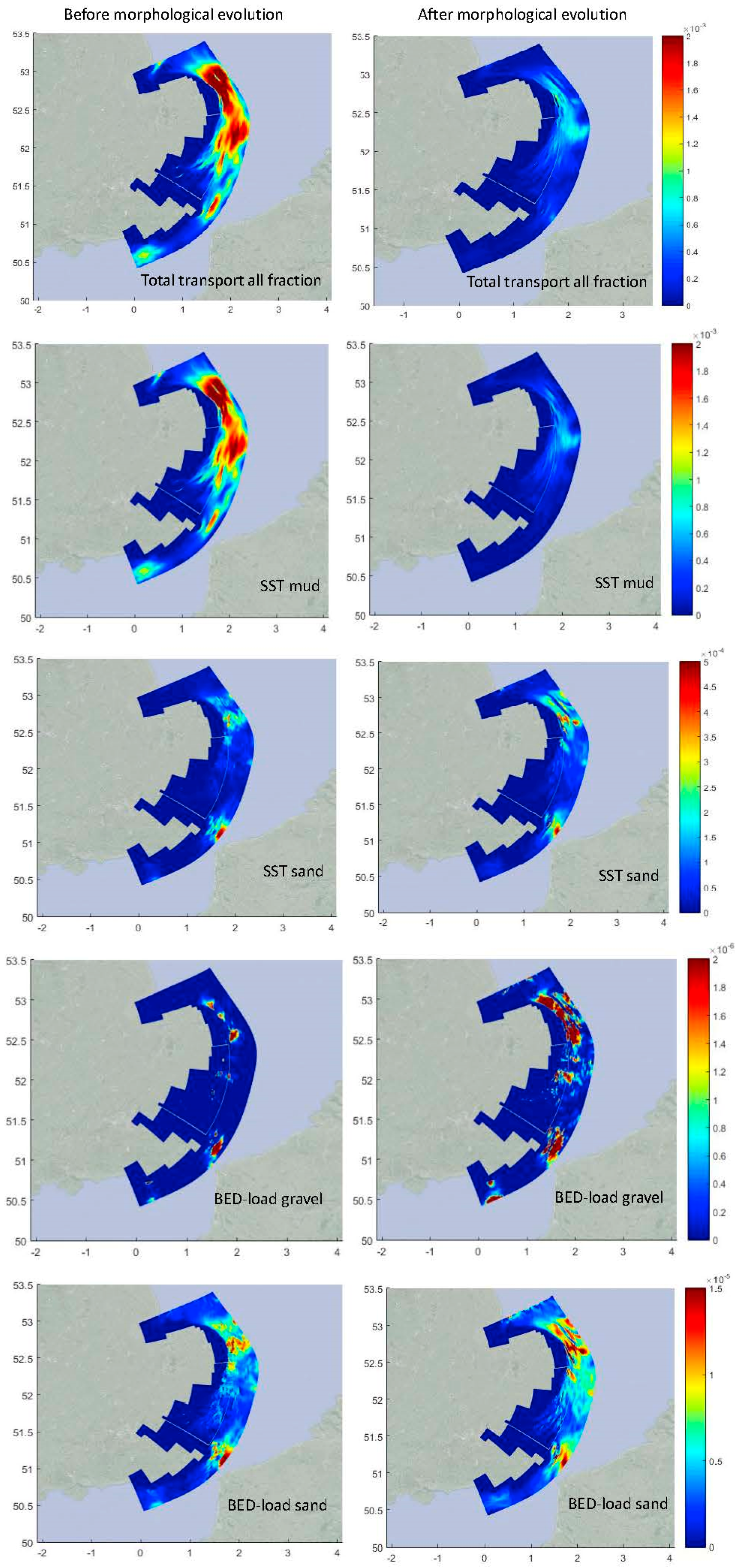
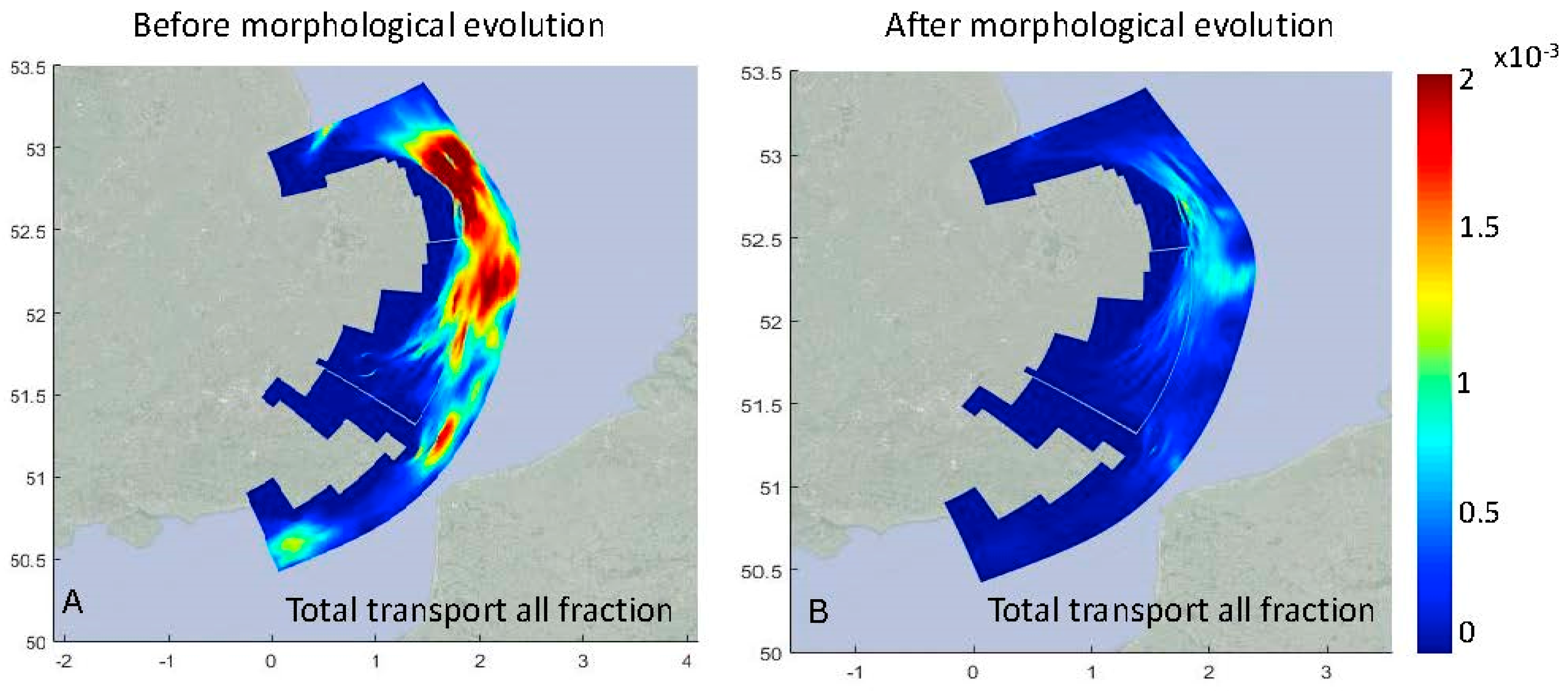
Net transport values significantly decrease as the simulation progresses; indeed, the reduction in net transport occurring as a consequence of the morphological evolution of the system can easily be observed by considering the spatial distribution of the net transport before, and after, the century-scale morphological update (
Figure 4,
Figure A2). For the existing bathymetry (
Figure 4A) and for spring tide, maximum net transport values occur in the form of a continuous band in the east portion of the domain, followed by a patchier distribution near Dover, and Newhaven. Given the same hydrodynamic forcing, but a morphologically-updated bathymetry (
Figure 4B), the net transport largely decreases across the entire domain. Higher net transport values remain in the form of thinner bands around the Norfolk banks, and for areas below Lowestoft, while the net transport in the majority of the domain largely declines, or even vanishes. The net transport values are dominated by the suspended sediment transport of mud, as the transport of the other sediment fractions is significantly smaller i.e., one order of magnitude smaller for sand, and two orders of magnitude smaller for gravel (see
Figure A2 for the residual transport of all sediment fractions). Specifically, there is a clear decreasing trend for the suspended sediment transport of mud, which dominates the total transport; the decrease in suspended sediment transport of sand and changes in bed load transport are more unclear (
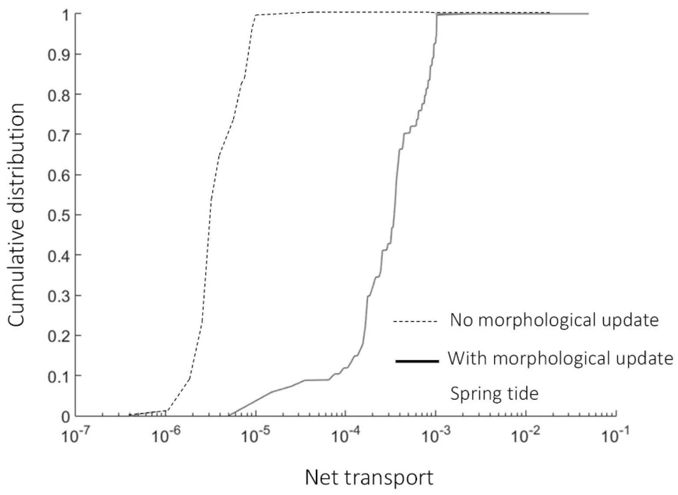
Figure A2). Across the entire area, the distribution of residual transport values is, on average, more uniform once the morphological changes have taken place, as it can be noticed from the cumulative distribution of the net transport values (
Figure 5); the dashed line in
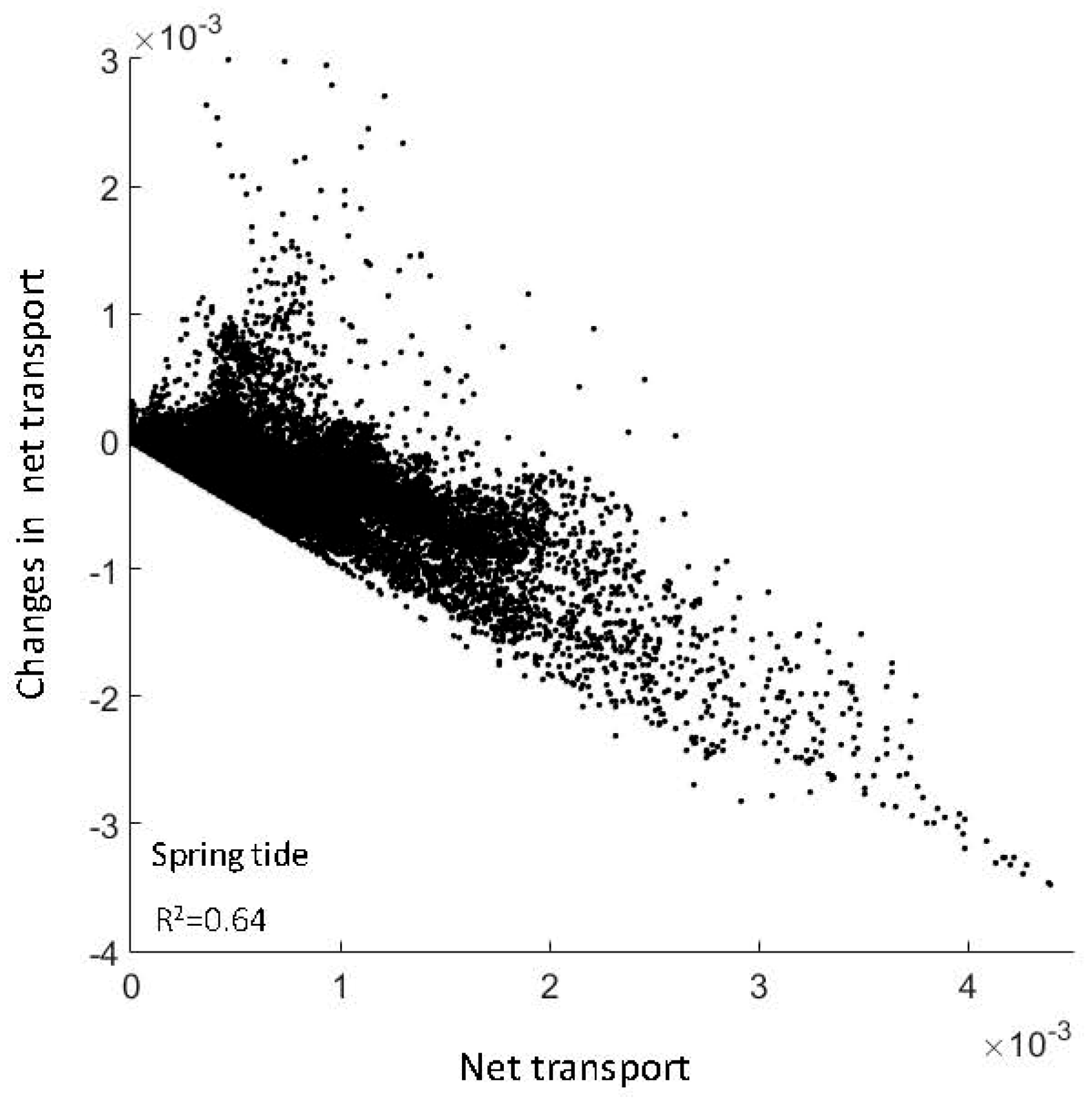
Figure 5 represents the percentage areas, with a given net total transport for the morphologically updated case, and this is significantly narrower and left-shifted with respect to the solid line (no morphological update). Magnitude differences between the residual transport before and after the morphological evolution of the system are then well correlated and largely increase with initial net transport values (
Figure 6).
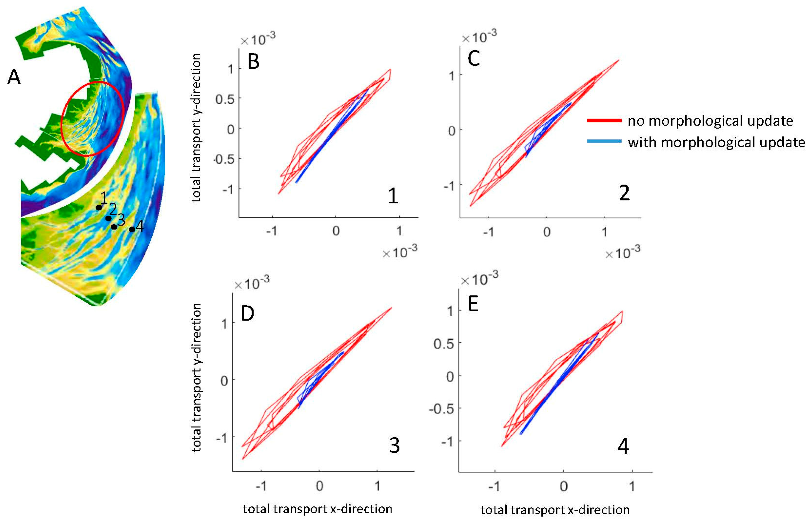
As a consequence of the morphological evolution of the system, transport patterns for the channels within the Thames region are also subject to significant variations.
Figure 7 presents total transport over time for four points within the Thames channels (
Figure 7A). For all locations, the orbital patterns become much narrower, and with a clearer preferential flood-ebb direction with respect to the initial configuration. This can be explained through an enhancement of the sandbank features in the area, which force the flow through a preferential direction. For all locations, the instantaneous total transport also decreases.
Given the same hydrodynamic forcing, the results presented above are relevant to the impact of the century scale morphological changes on the sediment transport patterns of the system.
Figure 8 and
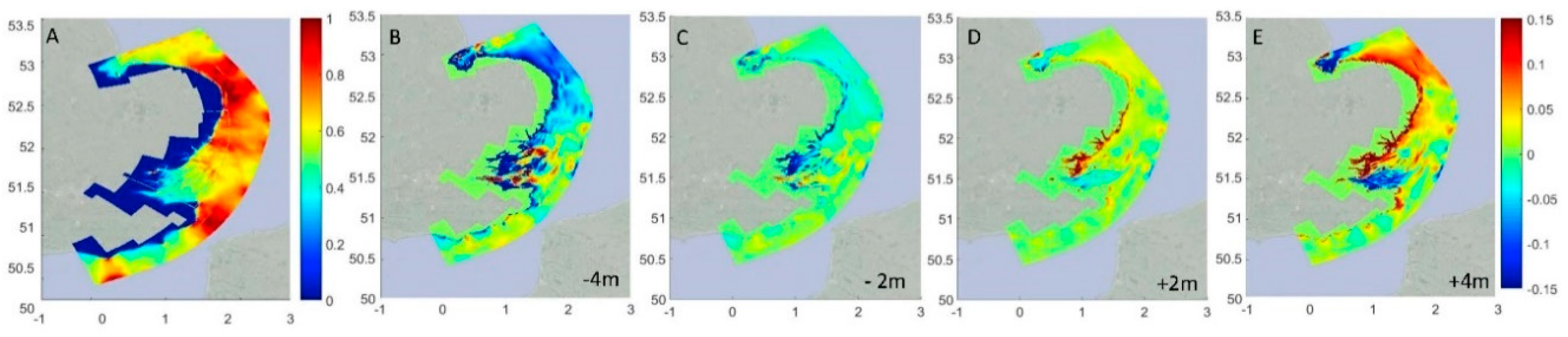
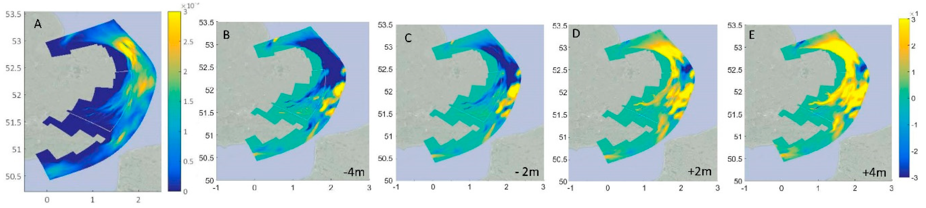
Figure 9 illustrate instead changes in residual currents and residual transport for the same input morphology, but different sea level values. In
Figure 8, the first panel represents residual currents under existing sea level values, while panels b-e represent differences in residual current magnitudes caused by sea level variations. Significant reductions in the mean sea level (−2, −4 m with respect to original values) correspond to a large decline in residual currents across the north portion of the domain (
Figure 8B,C). Also, the larger the decrease in sea level, the weaker the residual currents. Contrarily, increasing sea level mostly leads to large increments in residual currents, especially in the northern portion of the domain, though a decrease in residuals is observable in the southern portion of the Thames (
Figure 8D,E).
Sea level variations are also associated with changes in the net sediment fluxes (
Figure 9). Decreasing sea level causes a decrease in the net transport across the northern portion of the domain; in comparison, variations in total transport within the southern region are relatively small, with the upper portion of the Thames Estuary being the mostly affected. As the water level increases, a large increase in the net transport can be observed in the northern portion of the domain, and within the upper portion of the Thames Estuary; the southern portion of the domain shows instead relatively small variations. The trend of the system can be explained by considering that increasing sea level generally causes an increase in tidal prism values and faster propagation of the tidal wave, which in turn intensifies the tide-driven bed shear stress [
6,
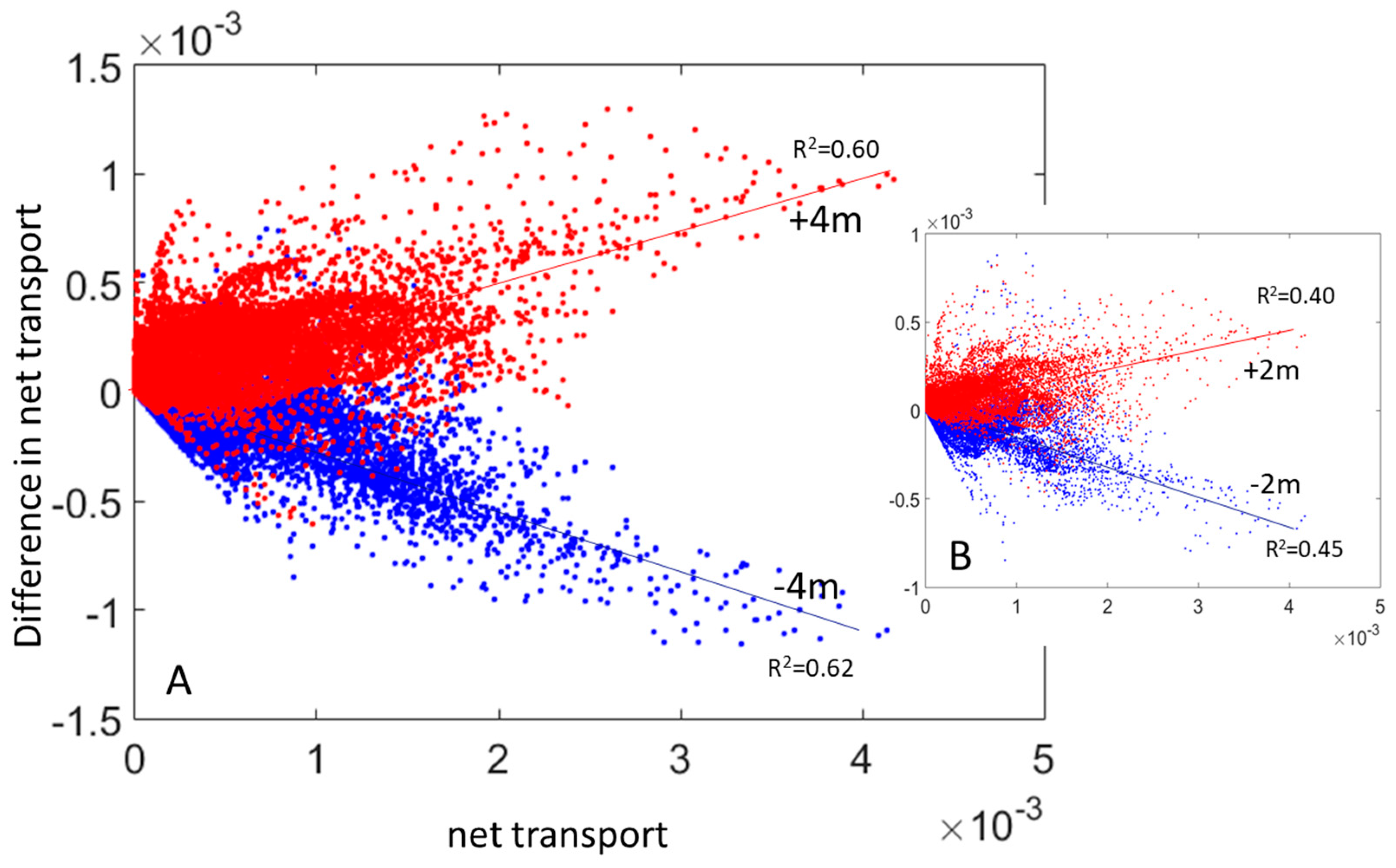
67]. Furthermore, similar to what has been shown for the variations in net transport connected to the 100-year morphological update of the domain, the variations in net transport, induced by water level variations, correlate well with the initial net transport values, especially when sea level changes are the highest. This suggests that the areas, which are most affected by variations in sea level, are the ones where the initial net transport is the highest (
Figure 10).
5. Discussion
In this theoretical contribution, the influence of morphological changes, and sea level variations on the residual transport patterns of the South East England, have been investigated using a hydrodynamic and sediment transport model. The results suggest that century-scale morphological changes induced by tidal currents tend to steepen existing sand banks, especially in the Thames and in the northeastern portion of the domain, where sand-banks tend to become higher and new ones tend to form. For the northeastern portion of the study area, the coastlines adjacent to the accreting sand banks tend to partially erode, while no significant sediment removal from the coastline areas can be noticed for the southernmost portion. This trend is enhanced when sea level rise is present.
The morphological evolution of the system slows down in time, and by the end of the simulation, topographic variations dropped significantly with respect to the beginning of the numerical test (
Figure 3). The presence of a gradual increase in mean sea level initially accelerates the morphological evolution of the system; the bathymetric changes, however, gradually attaining similar plateau values as those without sea level rise.
The net transport of sediments largely decreases as a consequence of the morphological updates (
Figure 4B). Indeed, changes in net total transport interests large parts of the domain, especially the Northeast portion, where the net total transport is lowered, and only maintains maximum values corresponding to the no-morphologically updated configuration within relatively small and patchy areas (
Figure 4). Specifically, the stronger the initial net transport, the larger the dampening effect induced by morphological changes (
Figure 6).
The results in relation to the morphological evolution of the system and sediment transport patterns suggest that, under tidally dominated conditions, the system might tend toward a dynamic equilibrium configuration, which is also attained when sea level rise is present. The idea of morphodynamic equilibrium has been mostly studied up to the scale of estuarine and deltaic systems. First empirical evidences in relation to the existence of a tidally-induced morphological equilibrium were about tidal inlets in the USA, showing a correlation between tidal-prism and inlets cross-sectional areas. The validity of this relationship was later extended to any location along individual tidal channels, when the tidal prism relevant to each specific cross-section was considered [
68]. Numerical models, and field data have then shown that, for funnel-shaped channels and estuaries, given an initial arbitrary bottom topography, the bottom evolves asymptotically toward an equilibrium configuration; this equilibrium condition is controlled by the temporal symmetry of the flow field, as suggested by the numerical results, as well as by field observations [
23,
25]. A formal equilibrium for tidal channel morphology has been only analytically found through rigorous simplifications of 1D models [
28,
69]. It has been also noted that this dynamic equilibrium condition is compatible with the higher order contributions of settling and scour effects to the channel profile, as well as with the fact that a real equilibrium condition is only asymptotically achieved and that for real scenarios an evolution of the system is still present due to variations into external forcing induced, for instance, by storms occurrence, or changes in sea level [
2,
24,
27,
70,
71,
72]. This manuscript supports the possibility to extend the morphodynamic equilibrium concept to systems up to a regional scale.
Given the same morphology, increasing sea levels cause an increase in residual currents and net transport near the coastline. Similar to other coastal systems, this can be explained by considering that an increase in water depth causes the tidal wave to propagate more easily, yielding higher discharge and increased velocity values [
27,
73,
74]. A decrease in sea level causes a large dampening of residual currents and residual transport within the Thames region, and especially in the northern portion of the domain; a reduction in sea level also generally causes a large decrease in net sediment transport.
Under the simplified modelling framework presented in this manuscript, the influence of wind generated waves has been neglected. However, wind waves enhance bed shear stress and sediment resuspension. Given the vertical structure of waves’ motion their impact is expected to be especially pronounced in the shallower areas, and wave action can alter the tidally-induced morphological changes [
32]. Van der Molen [
75] analyzed the relative dominance of tides versus storms for net transport in the North Sea and showed that, tides dominate the net transport along the East coast of the UK and in most of the Southern Bight.
Our results represent a first incremental step for the understanding of changes in sediment transport patterns with morphology. Future efforts will include both hydrodynamic and wave forcing, which together with the present contribution, will allow the investigation of the relative impact and compound action of wind waves and tides. Our contribution currently illustrates the importance of coupled sediment transport and morphological models to effectively estimate the sediment transport along the different portions of the coastline, and also support the idea that morphodynamic equilibrium is extendible at a scale larger than the one for which it has been generally explored, i.e., estuarine scale.
Our results confirm that the dynamic behaviour of tidal systems are sensitive to changes in external forcing, such as sea level variations and morphological alterations. Such agents might disrupt the long term tendency of the system toward a dynamic equilibrium.
