Abstract
While Light Detection and Ranging (LiDAR) revolutionized archaeological prospection and different visualizations were developed, an automated detection of cultural heritage still poses a significant challenge. Therefore, geographers and archaeologists from Westphalia, Germany are developing automated workflows for classifying field monuments from special terrain models. For this project, a combination of GIS, Python, and Object-Based Image Analysis (OBIA) is used. It focuses on three common types of monuments: Ridge and Furrow areas, Burial Mounds, and Motte-and-Bailey castles. The latter two are not classified binary, but in multiple classes, depending on their degree of erosion. This simplifies interpretation by highlighting the most interesting structures without losing the others. The results confirm that OBIA is suitable for detecting field monuments with hit rates of ~90%. A drawback is its dependency on the use of special terrain models like the Difference Map. Further limitations arise in complex terrain situations.
1. Introduction
The use of airborne laser scanning in archaeology started almost 20 years ago. Since then, LiDAR revolutionized archaeological prospection and new visualizations were invented to ease interpretation of field monuments. In parallel, the need for automated workflows and classifications became evident to handle the growing number of datasets.
One of the first archaeological applications of LiDAR in Germany was performed by Sittler in Rastatt [1]. He successfully searched for Ridge and Furrow structures, digitized some of them manually, and carefully predicted that algorithms would be able to detect structures automatically. Later, Heinzel and Sittler [2] presented an automated approach using Pattern Recognition for the detection and delineation of single Ridge and Furrow structures. The evaluation with reference data produced accuracies up to 84%, depending on the complexity of the terrain.
In parallel, de Boer experimented with Template Matching to detect Burial Mounds in the Netherlands [3]. This technique slides a tiny digital terrain model (DTM, the template or window) over the DTM of a study area and calculates the correlation to the part that is currently covered by the template. The result is a raster with correlations at each position written to the corresponding pixel. The highest pixel values of this raster are considered as hits. De Boer used multiple templates of different sizes and was able to detect most of the reference mounds. In the end, the research was not continued due to too many false positives [4].
Another project to detect field monuments using Template Matching was undertaken by Trier and a Norwegian research team. In multiple publications, they demonstrated how to detect pits and similar structures like Burial Mounds or Charcoal kiln sites [5,6,7]. An example from Germany is Schneider et al., presenting a workflow for detecting Charcoal kiln sites using Template Matching as well [8].
Most recently, Freeland et al. provide an example of an automated detection of mounds in the Kingdom of Tonga [9] and Cerrillo-Cuenza presents a workflow for detecting mounds in Spain [10]. In 2018 and 2019, Davis et al. developed and compared workflows for the detection of mounds in South Carolina [11,12].
Up to now, however, not all field monuments are covered and furthermore no attempt was made to adapt the variety of methods to the province of Westphalia, Germany, which has a rich archaeological record including monuments from the Stone Age until World War II (Figure 1). Therefore, the project presented here aims at a provincewide detection of frequently appearing field monuments like Burial Mounds and medieval fields, improving knowledge of Westphalia’s historic landscapes and supporting preservation; e.g., medieval fields are strong indicators for lost settlement that often are completely invisible in the terrain and help to reconstruct spatial distribution of settlements in different epochs.
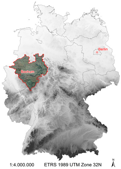
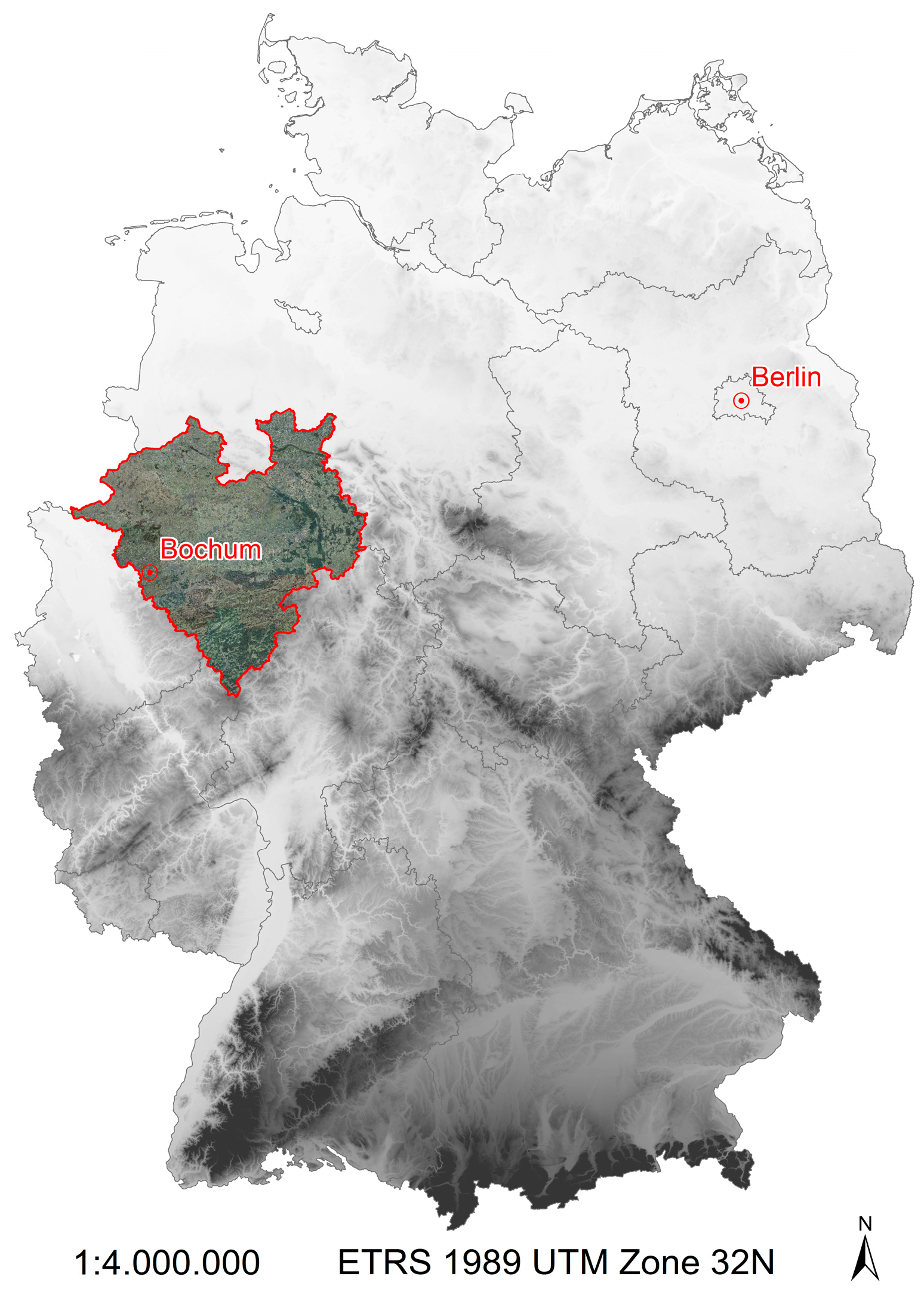
Figure 1.
Location of Westphalia (red) in Germany along with the cities of Bochum and Berlin for reference. Data source: SRTM & [13].
Westphalian archaeologists are limited regarding funds to spend on projects like this. Therefore, as a secondary objective, this project examines the potential of the currently only available LiDAR data source for automated classifications using OBIA. The quality is far away from today’s standard but it is for free, covers the whole province and is presumably precise enough for detecting the desired structures.
This article presents the initial steps of the project, in which workflows are developed and tested. It will be demonstrated that the combination of OBIA and a simple terrain visualization is suitable for the detection of different types of field monuments. These workflows are supposed to be finally used for a provincewide detection of field monuments.
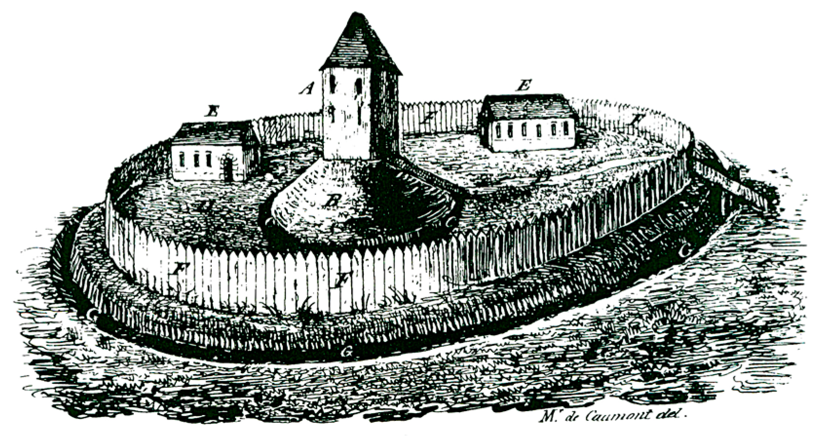
Three types of field monuments are considered. In the beginning, Motte-and-Bailey castles were used to investigate the potential of OBIA for the classification of complex structures. A Motte-and-Bailey castle is a medieval fortification that consists of a mound and a surrounding bailey. The former usually carried a fortified building and the latter was the place for other buildings of varying purposes (Figure 2) [14]. Today, in most instances, only the motte and its surrounding ditch are preserved in varying shapes and conditions (Figure 3). Other common field monuments are areas with Ridge and Furrow structures (Figure 4). A single ridge is the remnant of an early medieval field that was just a few meters wide but hundreds of meters long [15]. The third type of field monument is the Burial Mound. These mounds were common in the Bronze Age and the Iron Age and are preserved quite often.
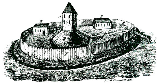
Figure 2.
Motte-and-Bailey castle [14].
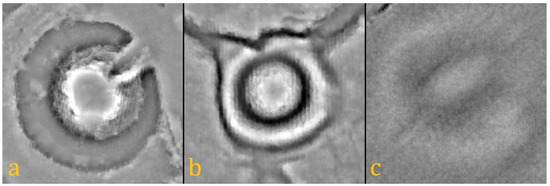
Figure 3.
Overview of the different castles from the reference data: (a) Borken, (b) Paderborn, and (c) Warburg [13,16].
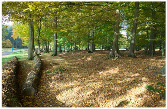
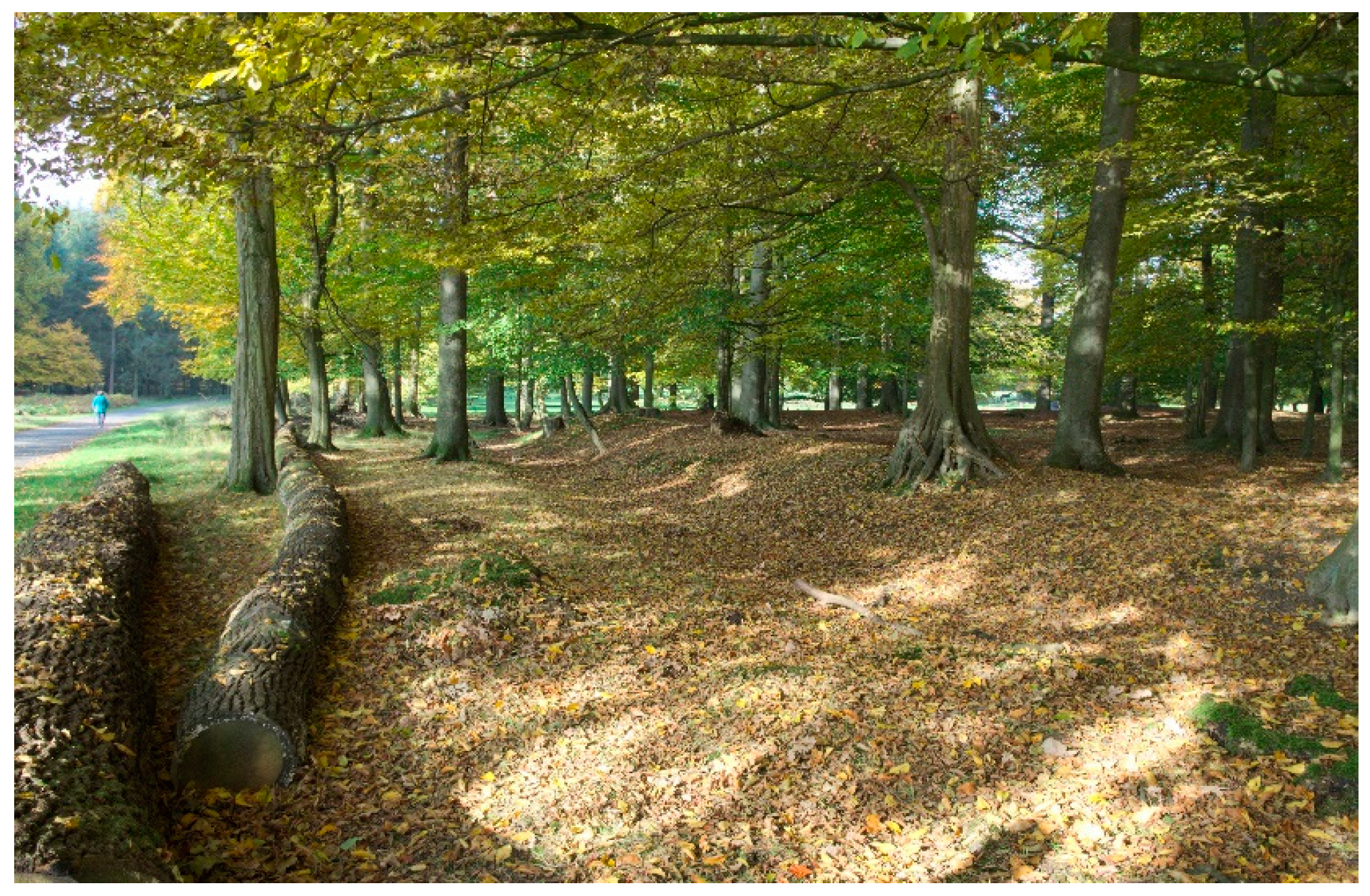
Figure 4.
Ridge and Furrow area in Dülmen.
Although new monuments are searched systematically, there are still many field monuments hidden in the terrain. Looking at the size of Westphalia, the need for automated approaches becomes obvious. It has an area of about 21,000 km2, of which ¾ are unsealed and therefore suitable for archaeological prospection. In northern Westphalia, these areas mostly consist of agricultural land, whereas in the southern mountainous region forests are dominating the landscape. Pastures and some minor land use classes are present all over Westphalia.
2. Materials and Methods
Archaeologists in North Rhine-Westphalia (NRW) benefit from the Open Geodata principle of the provincial government, which provides up-to-date and continuously updated spatial data for free [17]. Table 1 provides an overview of the datasets that were used in this project so far.

Table 1.
Overview of the LiDAR datasets.
The LiDAR datasets for the detection of Motte-and-Bailey castles and Ridge and Furrow areas were acquired between 2008 and 2010 and provided as filtered point data in an irregular distribution with a point density of 1–4 pt/m2. The data for the detection of mounds were acquired in 2016 and provided online [17] as filtered point data in an interpolated regular grid with 1 pt/m2—these point data can be converted to DTM without interpolation.
Additionally, a digital land use model (DLM) containing information about the current land use as point, line and polygon features is used [11,17]. From this dataset, polygons representing unsealed areas were extracted once and merged into a ‘positive layer’, to which the search is limited. This avoids misclassifications in areas where no monuments can be preserved, e.g., in settlements or mining areas (Figure 5).
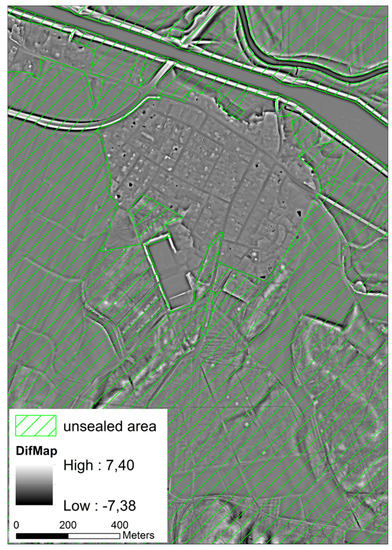
Figure 5.
Difference Map of a part of the investigation area in Haltern. The search is limited to the areas that are unsealed (green). The others, primarily settlements, are not considered [13].
For the development and evaluation of the classification algorithm, reference data were taken from FuPuDelos, the official database of archaeological records, maintained by the Westphalian archaeology [18]. There are three things to consider when working with this dataset:
(1) To ease evaluation of the Burial Mounds, a GIS will be used to flag all results having a reference point feature inside as true positives. This requires the points to be very precise, but some are offside up to a few meters due to imprecise recording in the field. They need correction based on visual inspection of the terrain model, which is done manually for all monuments in the investigation area. (2) Some monuments that are not protected by law were destroyed between their record and the acquisition of the terrain model. They are not present anymore and therefore cannot be classified. The reference points corresponding to destroyed monuments were removed from the dataset to avoid their impact on the classification. (3) The dataset tends to be incomplete and contains some records that were not yet confirmed in the field. This must be considered in the evaluation. Therefore, results are also inspected visually in the terrain models and aerial photography.
To evaluate the classification, especially with the Burial Mounds, results are interpreted as true positives (TP) if they are present in the reference dataset. For the sake of simplicity, results that are absent are false positives (FP), although a few of them might be revealed as new findings. Therefore, all FP were interpreted visually based on different terrain models and aerial photography. Even without inspection in the field, some of them are most likely new discoveries—these are called new positives (NP). Finally, evaluation and interpretation are difficult and therefore the workflows are supposed to lead the interpreter’s focus to the most promising features. In this context, the authors agree that the final interpretation still cannot be done by a computer (e.g., Sevara et al. [19]).
In this project, two approaches are considered. On the one hand, discrete field monuments are classified by tracing their shape. In doing so, castles and mounds are not only classified binary as true or false, but furthermore by their degree of erosion in multiple classes, e.g., to what extent they are leveled or stretched by farming activities (Figure 3c). This is a similar result organizing approach to that of Trier et al. [6].
In contrast to binary classifications, it is not necessary to optimize the algorithms towards high completeness or high correctness. Full completeness is guaranteed by the fact that the classes are derived by the worst preserved reference monuments. At the same time, the classes containing well-preserved results show high values of correctness. Their results are more likely to be true and can be interpreted at first. The drawback is that evaluation becomes difficult since calculating reasonable values for an overall correctness and completeness is hardly possible.
On the other hand, tracing the shape of areal monuments, e.g., Ridge and Furrow areas, is difficult if single elements looks like nonarchaeological structures. Therefore, the second approach is not to find every single ridge or furrow but to tag the location of the area by highlighting objects indicating an area of similar structures.
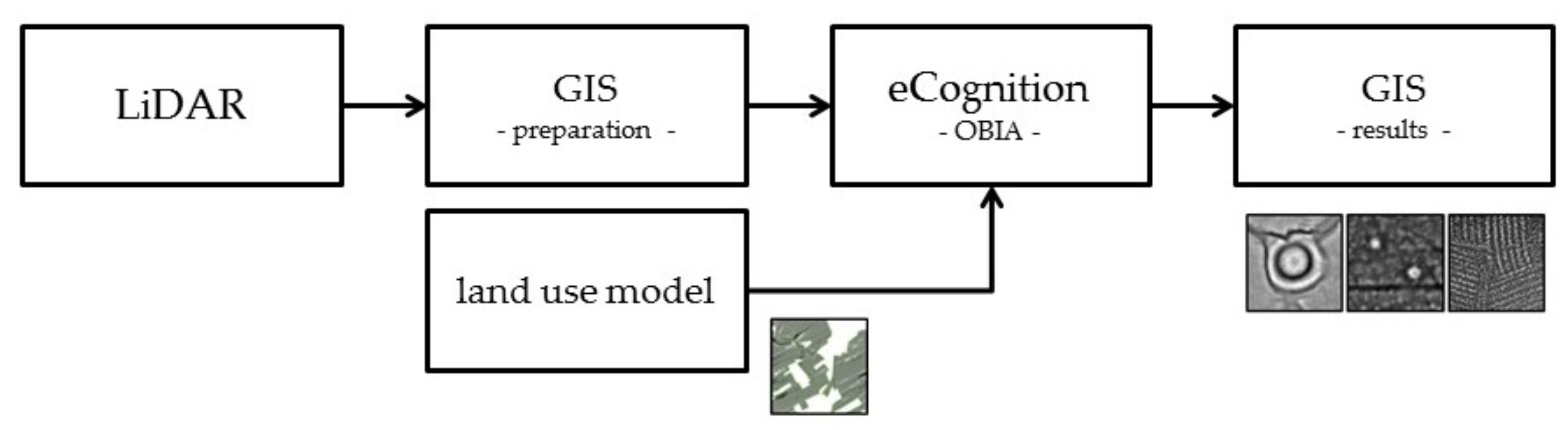
The workflow (Figure 6) starts in a GIS with the calculation of the desired visualization(s) and ends in the same place with the interpretation. Just as important as an accurate classification is an easy access to the visualizations and a user-friendly workflow. Therefore, an ArcGIS-tool was written in Python that is designed to work with the mentioned LiDAR data. It is capable of calculating different visualizations, currently a conventional DTM as well as the special visualizations Difference Map (DM) and Local Relief Model (LRM) that were both invented by Hesse [20]. The latter two exclusively show the microrelief, which is essential for a classification using OBIA (see below).

Figure 6.
Overview of the general workflow for the detection of field monuments [13].
For the classification, OBIA, implemented in eCognition Developer by Trimble, was used. This technique does not classify single pixels, but objects representing homogeneous areas within an image. In a DTM, they correspond to areas of the same height. Objects are generated in the initial segmentation step that has three adjustable thresholds: Most importantly, the scale parameter defines the final size of the objects. Adjustments are to be done very carefully to represent the real-world object as best as possible. The following two parameters describe the homogeneity of the objects: The shape parameter defines how much the algorithm takes the shape of the emerging object or the spectral values of its pixels into account. Finally, the compactness parameter defines the smoothness of an object border, which is a relation between length and width of an object and its area. The segmentation starts with converting every pixel into a single object and then iterates over the objects, merging the current one with the most similar neighbor. This is done until the adjusted thresholds are reached [21]. The segmentation is perfect when the object borders match the borders of their corresponding field monuments.
Afterwards, statistical values (features) are calculated for every object. Some of which refer directly to the object (e.g., length and width) and some to its neighbors (e.g., rel. border to brighter objects). From these, the user can choose features to describe classes. This is the advantage over pixel-based approaches because objects can be seen in a relation to their neighbors and therefore be discriminated by their location, which is essential for the detection of field monuments. In terms of OBIA, remnants of a Motte-and-Bailey castle can be described as a local maximum (the motte) or as an object completely surrounded by darker (lower) objects, which is in close proximity from a ring-shaped local minimum (a ditch surrounding the motte). Up to now, three rulesets where developed that run fully automated and export the classification results to GIS-compatible shapefiles.
Although OBIA does not ‘see’ an object in the way the human eye does, it nevertheless benefits from special terrain visualization like the DM or the LRM that were originally developed for manual interpretation. In this project, the DM was preferred over other Visualizations because of its excellent ratio of benefit and calculation effort. Calculation is done in two simple steps using a GIS: At first, the terrain model is smoothed using a low-pass filter, which removes the microrelief while preserving hills and valleys. The Difference Map is then calculated by subtracting the smoothed DTM from the initial one, only preserving the microrelief with its small-scale features [20]. Because hills and valleys were removed by the subtraction, the contrast increases significantly but most importantly, all monuments appear in a leveled situation because slopes are removed as well (Figure 7).

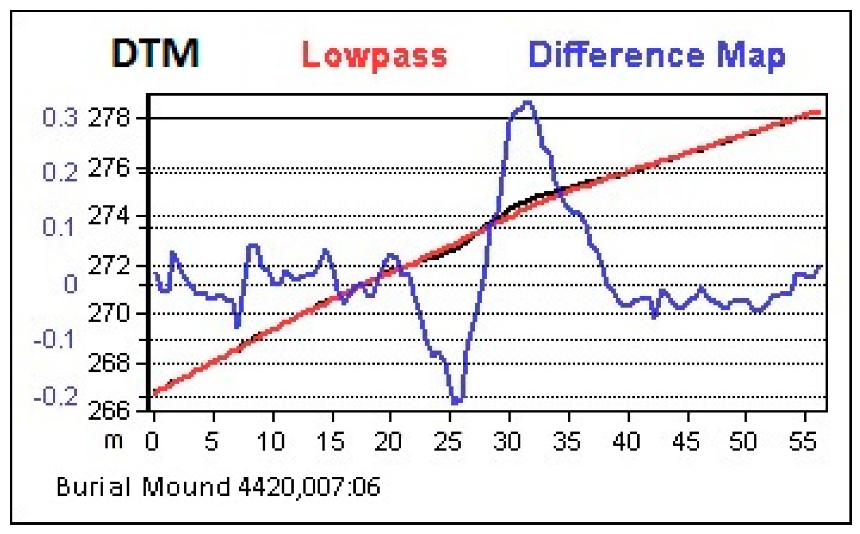
Figure 7.
Profile graphs of a Burial Mound in a digital terrain model (DTM) (black), a smoothed DTM (red) and the final Difference Map (blue) [13].
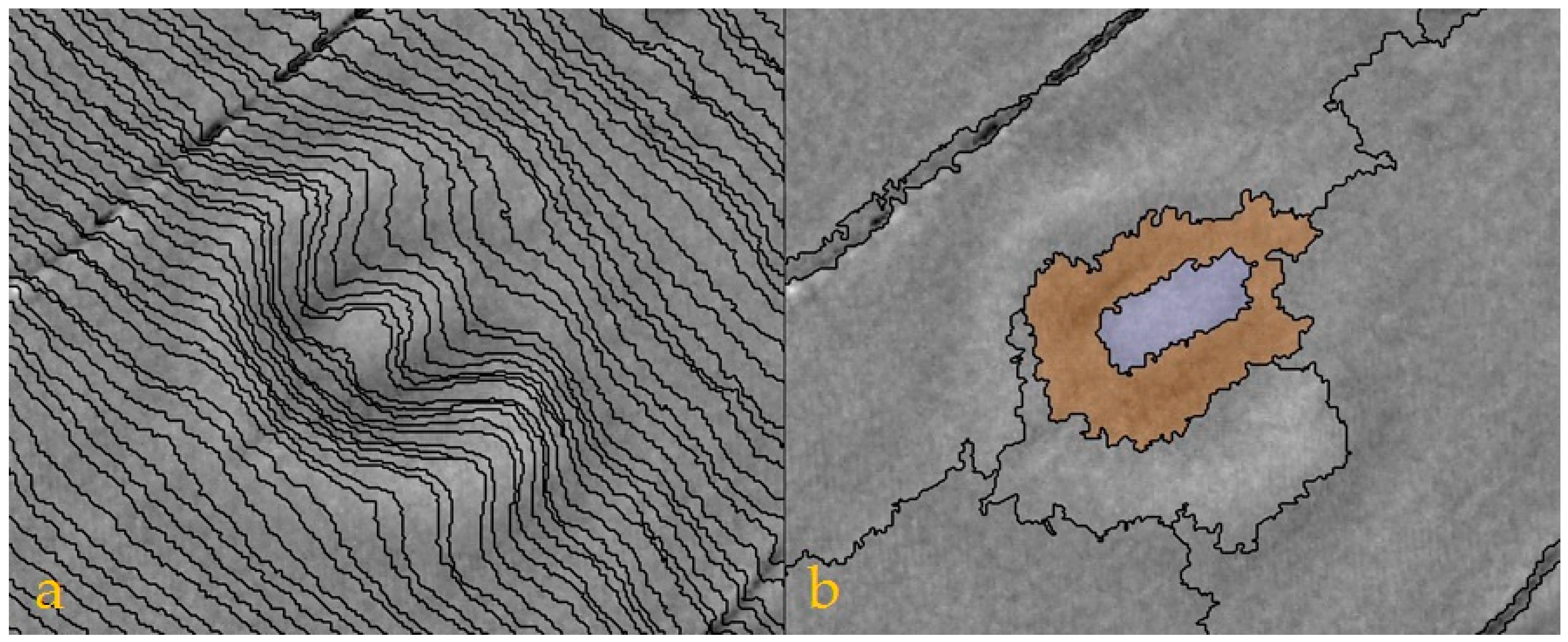
The latter is necessary because object borders in LiDAR datasets follow the contour lines making field monuments invisible to OBIA if they are located on a hillside. Figure 8 demonstrates this issue as the castle on the left side cannot be detected. On the right side the hill is removed and motte and bailey stand out against the surrounding area even though they are almost eroded completely.
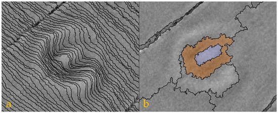
Figure 8.
Difference Maps of a highly eroded Motte-and-Bailey castle on a hillside in Warburg with overlaying objects derived from a regular DTM (a) and from a Difference Map (b) [13,16].
A disadvantage of using a visualization like this is that the calculation will usually generate undesired structures as well, especially in complex situations like slopes (Figure 9). They are a problem for the detection of some field monuments and cannot be handled perfectly.
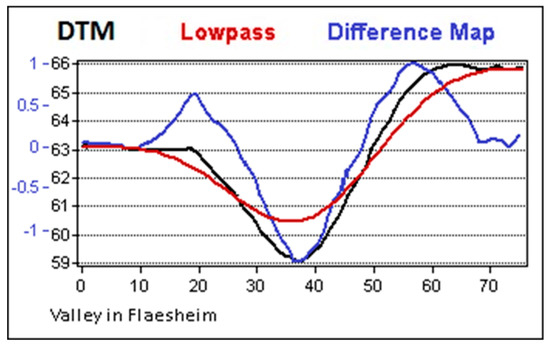
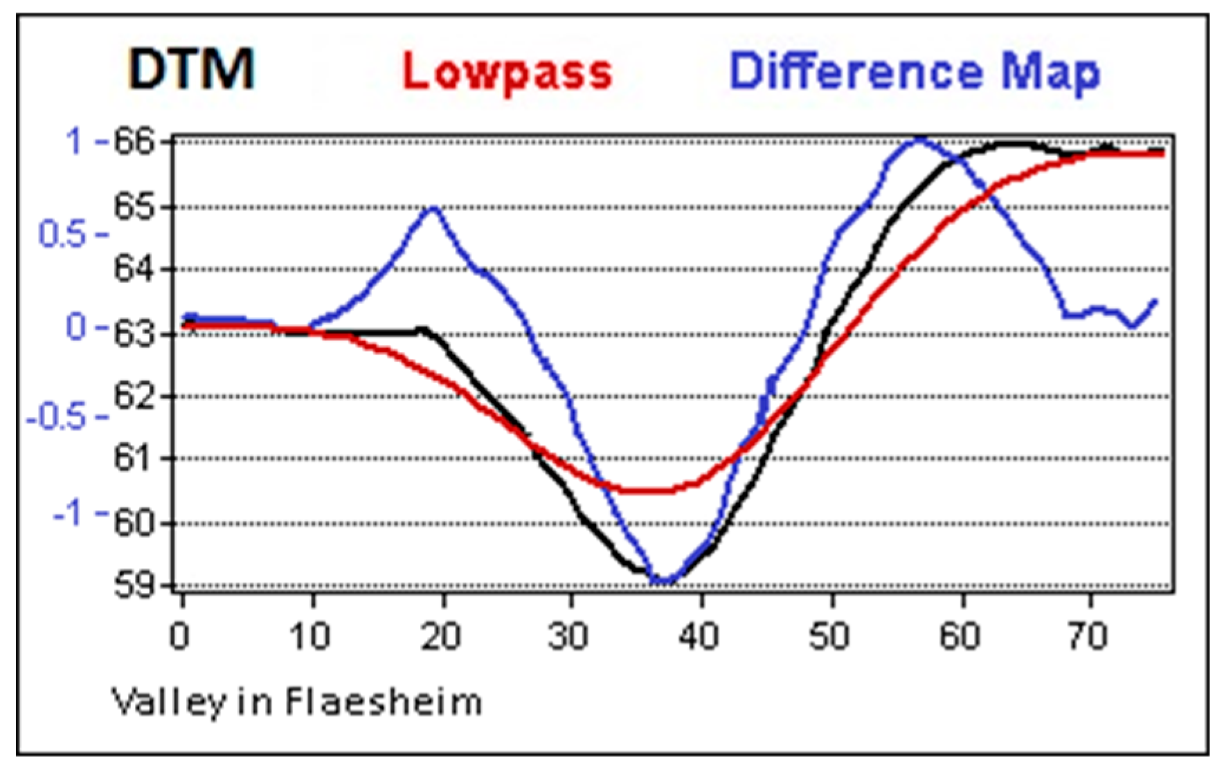
Figure 9.
Profile graphs of a valley in a DTM (black), a smoothed DTM (red), and the final Difference Map (blue) [13].
The next chapters will present the classification algorithms (rulesets). For the definition of class borders, software-internal statistics (features) are used. Based on the eCognition reference book [21], details are to be found below.
The following features describe the shape or extent of an object.
- Area equals number of pixels of an object. It can be converted into different measurements if a unit is available. In this case 1 px equals 1 m2.
- Border length/area describes the ratio of the border length to the area of an object. It is dependent on the shape and the size of object at the same time.
- Compactness is calculated by dividing the area of an object by its number of pixels. The ideal compactness equals 1.
- Density determines if an object is rather shaped like a square, which is the ‘most dense’ object, or like a filament. Calculation is done by dividing the number of pixels of an object by its approximate radius.
- Elliptic fit is calculated by comparing the object to an ellipse of similar size (area) and proportions (width and length). The overlapping area is then compared to the area of the object outside the ellipse. A value of 0 indicates less than 50% fit, whereas 1 indicates a perfect fit.
- Length/width: eCognition internally calculates two different length-to-width ratios, one of which using a bounding box. The smaller value is finally assigned to the object and helps discriminating between elongated and well preserved mottes.
- Max and Min pixel value provide the highest and the lowest pixel value of an object. When using a DM, it is representing the elevation of an object above ground level.
- Mean describes the average pixel value of an object.
- Roundness is calculated by subtracting the radius of the largest enclosed ellipse from the smallest enclosing ellipse of an object. The lower the value, the more similar the object looks to an ellipse, meaning that the roundness for the detection of mottes and mounds should be as low as possible.
- Shape index describes the smoothness of an object border. Low values are desired because they represent smooth borders.
- Standard deviation describes the homogeneity of pixel values of an object.
- Width is calculated by dividing the number of pixels of an object by its length/width ratio.
The second group of features describes the relation of an object to its neighbors. They help discriminating objects by their location and relation to others, which is essential for detecting many different types of structures:
- Distance to [class] describes the distance in pixels to the closest object of a specified class, measured from center to center.
- Number of [class] [distance] defines the number of objects in a specified class within a specified distance.
- Relative area to [class] [distance] is similar to number of. This value describes the area covered by objects of a specified class relative to the total area around the object within a specified distance.
- Relative border to [class] describes the percentage of the border length that an object shares with objects of a specified class relative to the total border length.
- Relative border to brighter objects [layer] determines if an object is surrounded by brighter (in terms of LiDAR: higher) objects. If the value equals 0, an object represents a local maximum.
2.1. Detection of Motte-and-Bailey Castles
For the development of the corresponding ruleset, three castles in very different conditions were considered. The first motte in Borken (Figure 3a) still carries a house from the 18th century [22] and is therefore in perfect condition. The second one—the Imbsenburg in Paderborn (b)—was destroyed at some point but is still in very good condition. The last one, located in Warburg, is almost completely leveled off by farming activities over the last centuries (c).
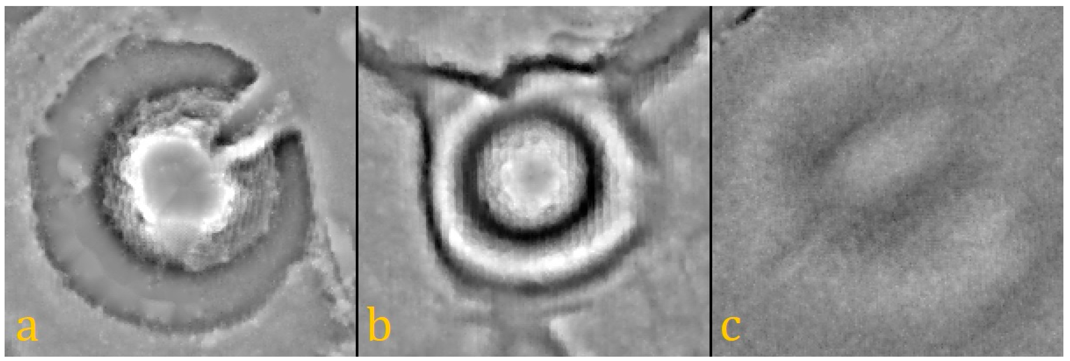
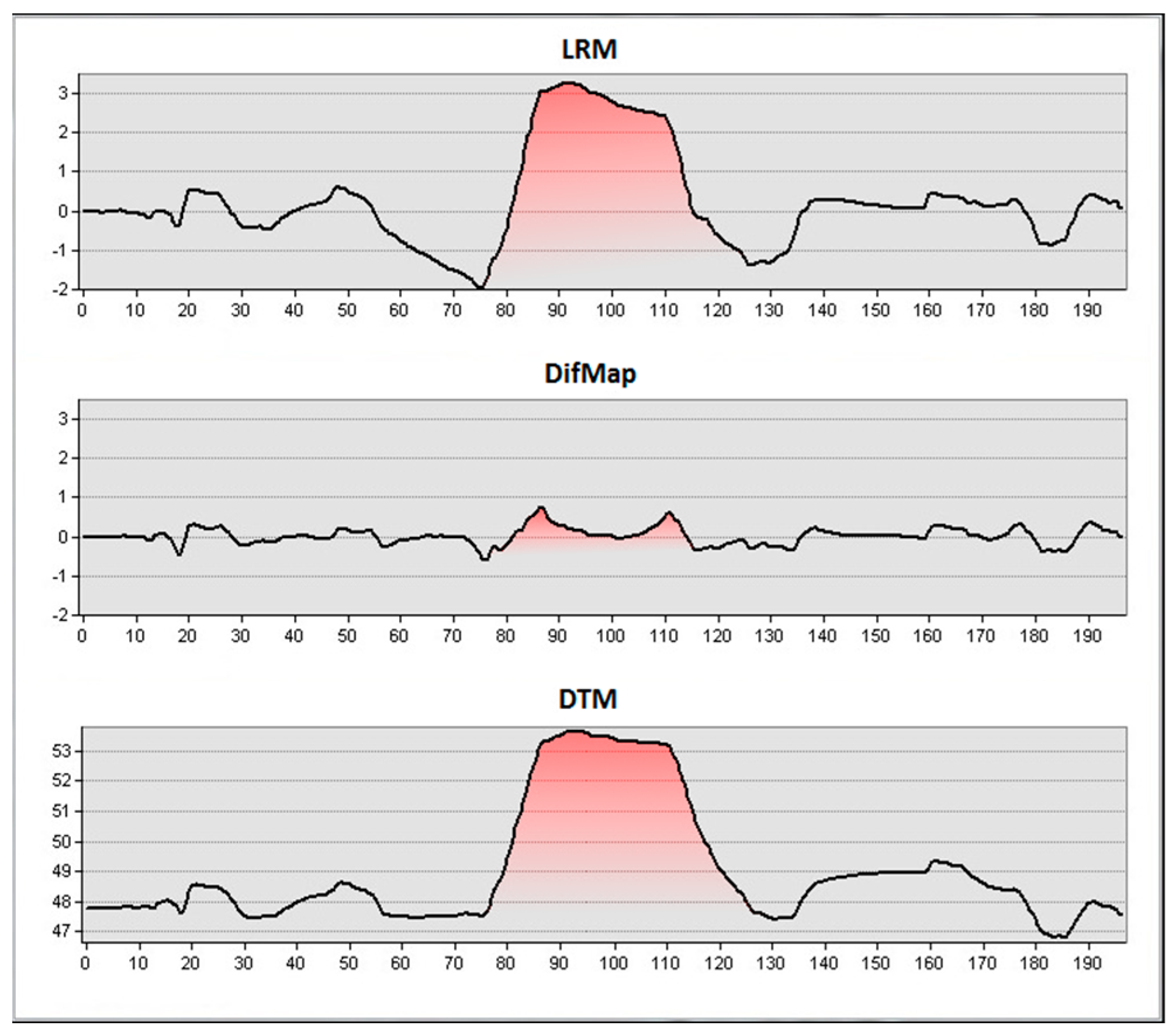
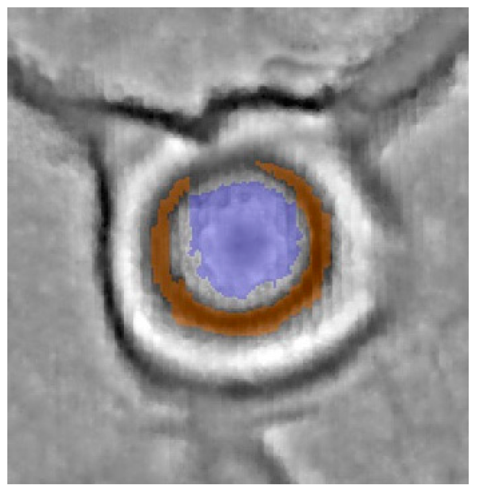
Looking at mottes (a) and (b) in Figure 3 again and comparing the profile graphs of motte (a) in Figure 10, another link between visualization and classification becomes obvious. In the DM, the border of the motte appears higher than its center and the motte becomes a ring (Figure 10, center). This is a result of the low-pass filter that starts flattening the mound from the edges towards the center, which has to be considered in the classification step because the surface of the mound is not homogenous enough to be represented by a single object.
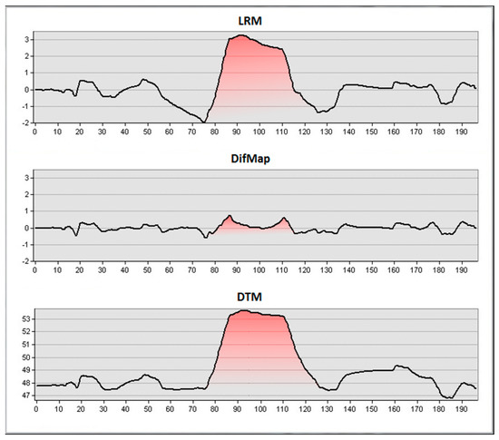
Figure 10.
Profile graphs of the motte in Borken in the LRM (top), Difference Map (DM) (center) and DTM (bottom). The motte is highlighted in red [13].
The first task was to find suitable settings for the segmentation that would work in all areas. After several tests, the settings 10/0.001/0.5 (scale/shape/compactness) were chosen to generate large objects, which strongly take into account the pixel values (the relative height) and are quite compact, with the following statistical values (Table 2).
Table 2.
Overview of the objects representing the real-life mottes and the derived class borders.
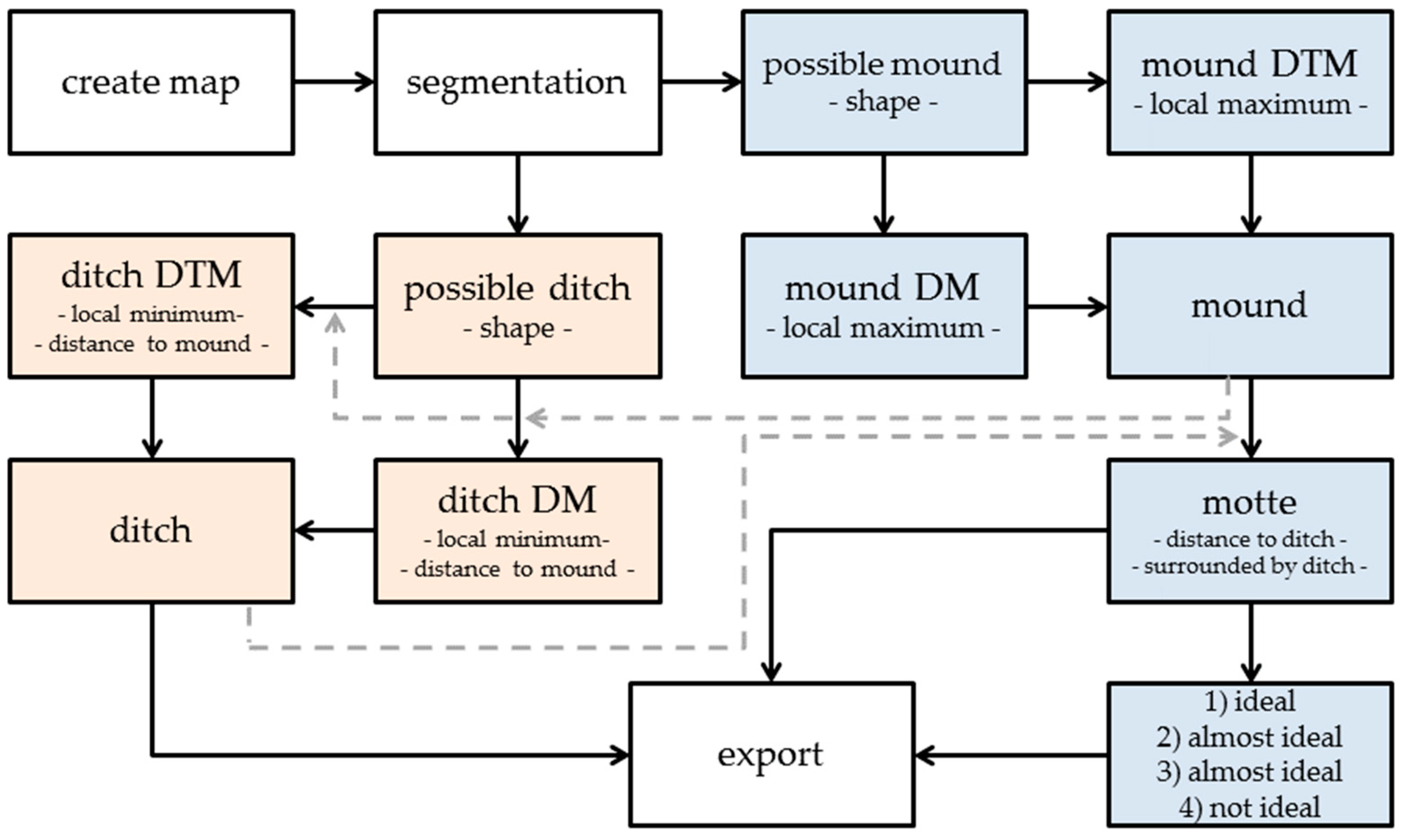
The classification (Figure 11) starts with the search for big mounds (the mottes, blue). All objects whose shape indicates a motte are collected in a class called possible mound. The values of the class borders are set in a way that allows the classification of more eroded structures and to avoid misclassifications as best as possible. In the next step, the software examines if an object is a local maximum and therefore still probably a mound (rel. border to brighter objects). Due to the mentioned problem resulting from the low-pass filter, the decision is based on both DM and regular DTM because in the latter a mound with pseudo structures is still intact. An alternative solution is to use a LRM but one wanted to avoid the calculation effort (see Figure 10 top). If an object is a local maximum, it is moved to a class depending on where it appears. These two classes get joined afterward in the class mound.
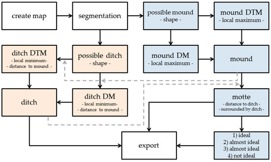
Figure 11.
Overview of the workflow in eCognition for the detection of Motte-and-Bailey castles.
Ditches are classified in almost the same way (red). At first, objects are classified as a possible ditch, depending on the shape statistics in Table 3. Secondly, objects that are a local minimum, either in the DM or the DTM, and that are located close to a mound object (<= 40 px), are classified in corresponding classes and finally joined in the class ditch. Vice versa, only those objects from the mound class are classified as a motte that are located in close proximity to an object in the ditch class (<= 40 px) and share at least 15% percent of their border with a ditch.
Table 3.
Overview of the objects representing the real-life ditches around the mottes and the derived class borders.
After the mottes are classified, they are sorted into subclasses by their appearance. Four classes were defined to cover all types that appeared so far as well as possible types in between (Table 4).
Table 4.
Overview of the classes that represent the mottes by their degree of erosion.
2.2. Detection of Ridge and Furrow Areas
For the development of the workflow two regions with extensive Ridge and Furrow areas were chosen. One of which is located in Dülmen, the other one in Höxter. Both are covered by forests and have an area of 8 km2.
Ridges and furrows appear in groups and trying to detect every single structure is not promising because the number of false positives would be too high. In addition, the reference dataset only contains the outlines of the areas. Therefore, it is again not possible to calculate reasonable values for an evaluation, which makes visual inspection necessary. The approach is to find single ridges and furrows (‘indicating objects’) that are surrounded by multiple similar structures, which makes them reveal themselves as a part of a Ridge and Furrow area.
This time, finding segmentation settings turned out to be much more difficult. The problem was that many segmentation settings were unsatisfying because the object borders did not follow the ridges or furrows in the way they were supposed to. After systematically testing, 5/0.001/0.5 (scale/shape/compactness) was chosen to work sufficiently. This setting is in a good balance between finding more eroded structures on the one hand and not producing too much useless objects on the other.
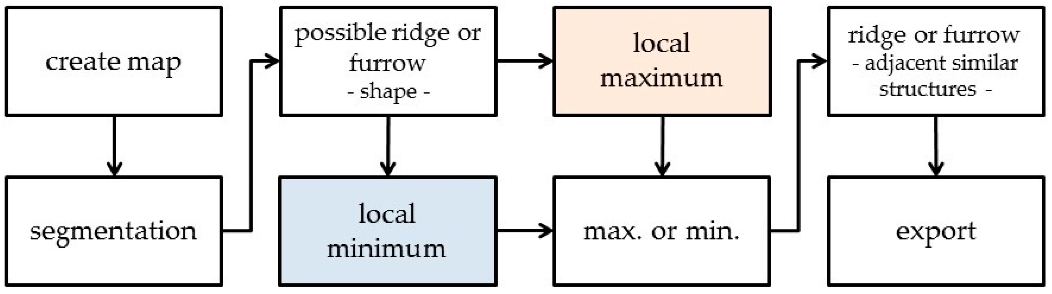
The first step after the segmentation is to find long and thin objects (Figure 12). The required statistics for an object to be classified as a possible ridge or furrow are listed in Table 5. As with the castles, the second step is to determine if an object in this class is a local maximum or minimum. Sorting in corresponding classes is again done with the rel. border to brighter objects criterion, this time using thresholds of > 80% and < 80%. After that, all minima and maxima are collected in max. or min. in order to determine which objects are surrounded by at least six objects of the same class in a defined area around the object. Besides, the classifier checks the distance to the next maximum or minimum and how much of the border of an object is shared with an object of the same class (Table 6). If an object meets all requirements, it is classified as a ridge or furrow and exported.
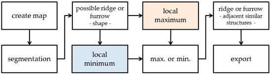
Figure 12.
Overview of the workflow in eCognition for the detection of Ridge and Furrow areas.
Table 5.
Description of the class possible ridge or furrow.
Table 6.
Description of the final class ridge or furrow.
2.3. Detection of Burial Mounds
The investigation area for the detection of Burial Mounds is located around the Haard, a hilly landscape close to Haltern. It mostly consists of forested areas with a decent amount of Burial Mounds in varying shapes and conditions as well as some other areas to test the robustness towards artificial structures.
Compared to the others, the detection of Burial Mounds is straightforward. In terms of OBIA, the task is to find round local maxima in the DM (Figure 13). Doing this is easy, but the drawback of detecting such a simple structure is a high number of false positives. This is minimized by using the landscape model to reject the results that are located in settlements and are therefore false.
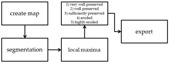
Figure 13.
Overview of the workflow in eCognition for the detection of Burial Mounds.
As mentioned above, mounds are not classified binary but in five classes depending on their degree of erosion. After finding segmentation settings (6/0.001/0.1, scale/shape/compactness) that sufficiently represent most of the (reference) mounds, class borders were derived by carefully looking at the statistics of the objects representing reference mounds (Table 7). The class borders become more restrictive as they describe more ideal mounds. This is done to separate these mounds from the others. The latter are collected in classes (4) eroded and (5) highly eroded and are therefore not lost. At first, all possible mounds are classified in class (5). After that, only those objects are classified further that meet the more narrow class borders of class (4). Then, it is the same procedure with classes (3) to (1) and therefore only the very best objects reach class (1).
Table 7.
Overview of the classes that represent the Burial Mounds by their degree of erosion.
3. Results
This chapter will present the results that were produced so far. They are structured by the monument that they describe.
3.1. Motte-and-Bailey Castles
Calculating a meaningful correctness and completeness for the detection of Motte-and-Bailey castles (Figure 14) is not possible, at least not at this stage, because the number of samples is too low. All three samples were detected, only in Paderborn a single false positive was classified. Testing some more castles, that did not influence the parameters, revealed some difficulties in the segmentation of distorted mottes and baileys. Other than that, shapes that differ from the three presented above need slight adjustments to be segmented. Additionally, this could be addressed by defining more classes. For further evaluation, a provincewide investigation needed to be carried out, which is not planned so far because the number of unknown castles is presumably not high enough. Nevertheless, the results show that a relatively simple algorithm in OBIA can detect complex multiobject field monuments like Motte-and-Bailey castles in different degrees of erosion, once useful parameters are found.
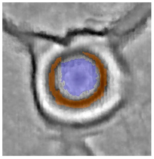
Figure 14.
Detected castle in Paderborn [13].
3.2. Ridge and Furrow Areas
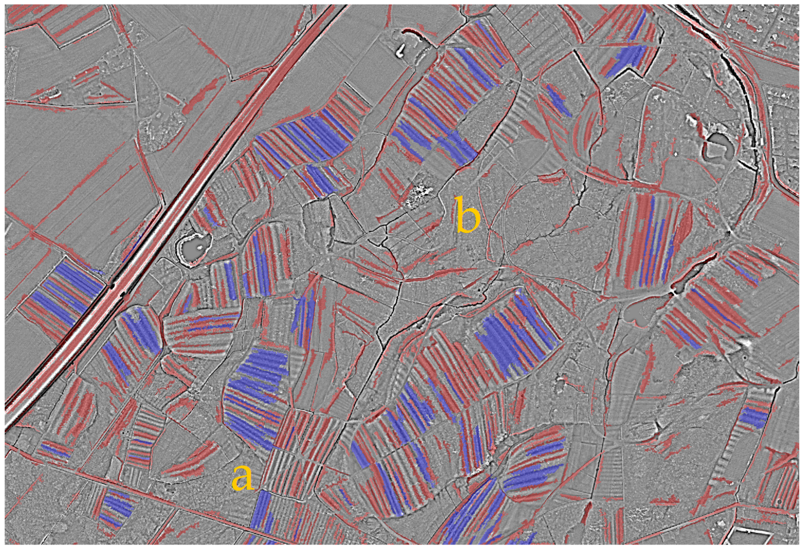
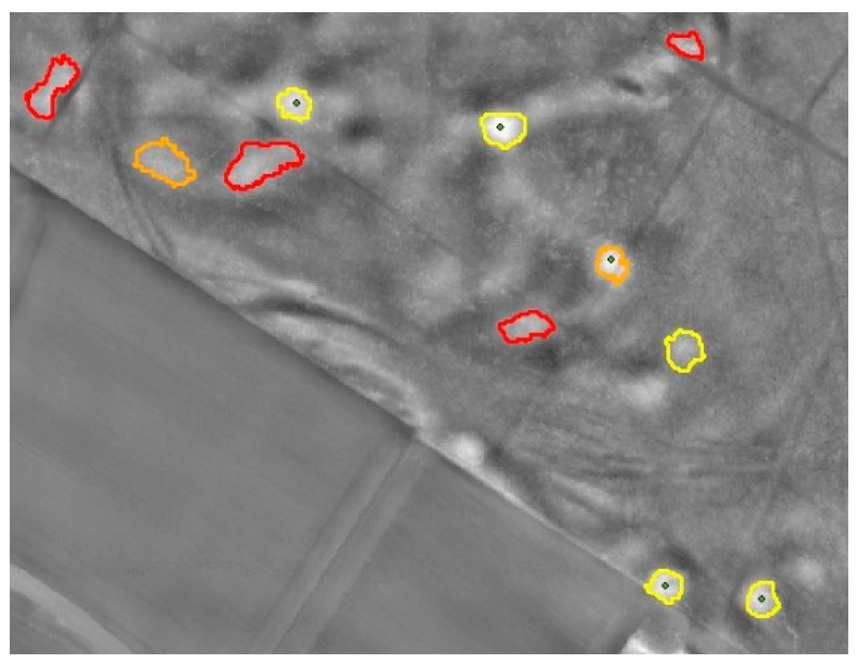
The results of the classifier for Ridge and Furrow areas are presented in Figure 15. Red structures represent single ridges or furrows who were left in max. or min. They do not have enough neighbors to be definitely part of a Ridge and Furrow area but nevertheless help to identify the blue ones. The latter are the important objects representing single ridges or furrows that have at least six adjacent objects of the same class around and can therefore be addressed as a part of a Ridge and Furrow area (class Ridge or furrow). These blue structures were found in every relatively big area. On the other hand, structures like modern drainages, which basically look like a sequence of ridges and furrows, were not detected—probably because their elements is too thin (Figure 15b).

Figure 15.
Classification result of the investigation area in Dülmen, overlaying a DM. The blue objects are ridges or furrows that have at least six adjacent objects of the same class and can therefore be addressed as a part of a Ridge and Furrow area. The red structures look like ridges or furrows in terms of shape and are a minimum or maximum, but do not have enough neighbors to be classified in blue [13,16].
According to the approach of finding these blue ‘indicating objects’, only one object is needed per Ridge and Furrow area. Therefore, having Ridge and Furrow areas being mostly colored red is fine, as long as there is at least one blue structure present. It is possible to identify more of the red objects as blue ones by lowering the threshold, but along with the number of blue structures, the risk to generate misclassifications rises as well.
Problems occur when ridges or furrows are cut (Figure 15a), which is caused by the scale parameter in the segmentation algorithm. To solve this problem, the whole process in eCognition would to be run again, starting with the time-consuming segmentation.
Other misclassifications occur if multiple paths run parallel to contour lines in hillside areas (Figure 16). The problem is that a sequence of path-slope-path-slope (etc.) looks like ridges and furrows, once the hill is removed in the DM. To address this, searching for slopes in the regular DTM might be a solution but the question arises, what happens to ridges and furrows that are located on a hillside and are oriented along the contour lines.
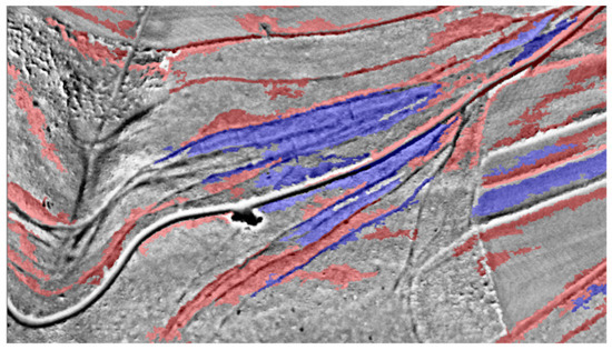
Figure 16.
Misclassifications in a hillside situation in Höxter in a DM [13].
3.3. Burial Mounds
Although completeness and correctness are not that meaningful as with binary classifications, Table 8 provides an idea of what is possible under good circumstances. The decreasing correctness is no surprise because the class descriptions get wider in order to find possible eroded mounds as well (Trier et al. 2015 observed the same with their confidence levels [6]). Completeness is 100% by definition because all 172 reference mounds defined the classes. Regarding the values, two things should be noted. On the one hand, some Burial Mounds were segmented insufficiently, meaning that it was impossible to generate objects with borders meeting those of the real-world mounds, and are therefore not included in the dataset with its 172 class defining mounds (see above). The lack of segmentation can be caused by a high degree of erosion, suboptimal segmentation settings or, most likely, a size differing significantly from the average. These mounds are missing in the classification and are therefore not included in the calculation.
Table 8.
Results of the classification of Burial Mounds in the investigation area in Haltern.
On the other hand, the reference dataset is probably not complete. Therefore, some of the false positives are actually unconfirmed and might be true, once they are interpreted or even excavated (the most promising false mounds are called new positives). The others are false positives until they are definitely interpreted as true or false.
Despite all these uncertainties, this method is still useful because the interpreter is able to interpret the classes with the most promising results (e.g., classes 1–3) at first and can eventually focus on the others or see the results in their relation to the others (Table 8).
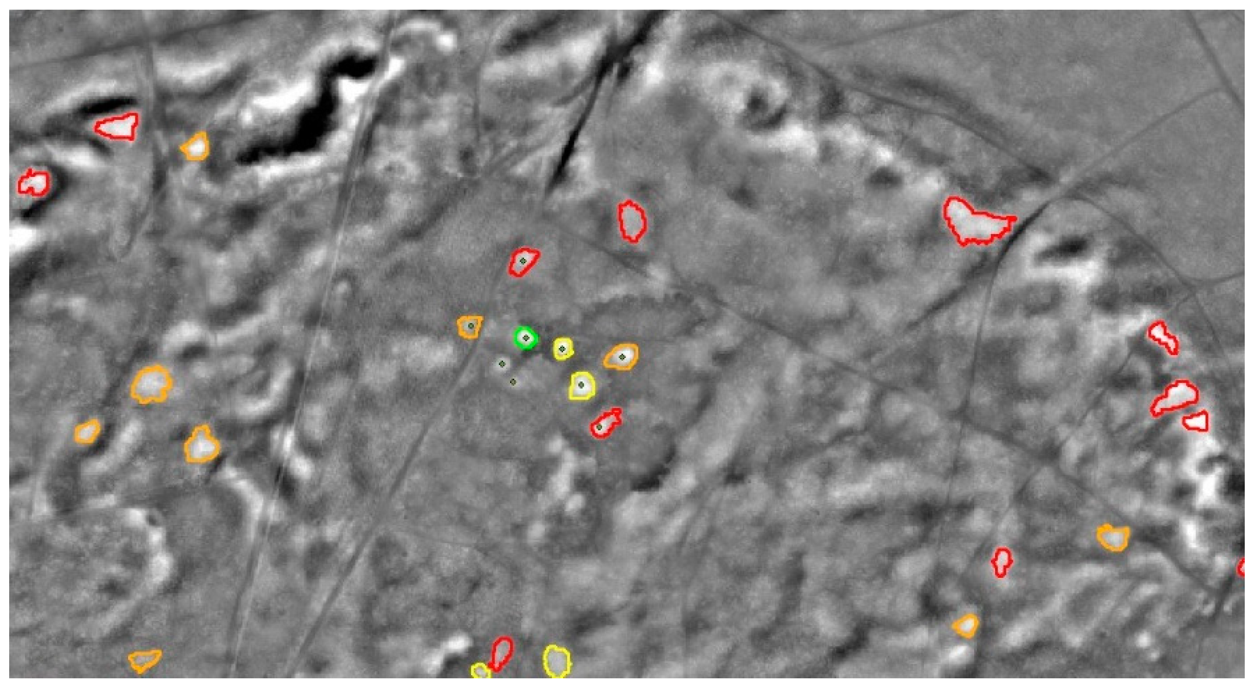
Figure 17 and Figure 18 present a subset from the mound detection area in Haltern. The decreasing correctness is displayed by the dominance of orange and red shapes, whereas more ideal shaped mounds are colored yellow and green. It is obvious that the classification works better in flat areas and has problems at edges, because the DM generates pseudo mounds where the terrain is more complex. Nevertheless, the results are useful and simplify the interpretation by highlighting probable monuments. In addition, Figure 18 shows a possible new mound (new positive, yellow) that was not included in the reference dataset (missing dot) and looks like its neighbors of the same class.
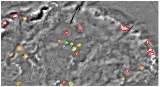
Figure 17.
Classification results of Burial Mounds in Haltern. Members from the following classes are presented (Table 8); 3 (yellow), 4 (orange), and 5 (red). Mounds with a dot are included in the reference dataset [13].
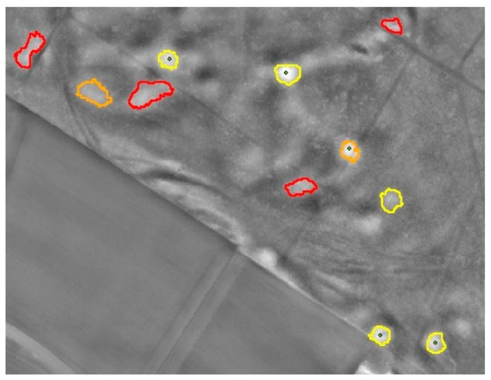
Figure 18.
Classification results of Burial Mounds in Haltern. Members from the following classes are presented (Table 8); 3 (yellow), 4 (orange) and 5 (red). Mounds with a dot are included in the reference dataset. The yellow traced mound on the right side without a dot inside is considered as a new discovery (new positive) [13].
Although detection of mounds produced useful results, there are some issues to be solved. A major problem is the variety of sizes, making it difficult to find segmentation settings that work for every size of Burial Mound. Multiple segmentation would be a way to address this. Another problem is that some mounds are classified in lower classes (e.g., 4 & 5) although their appearance is almost ideal. This sometimes happens due to only one outlying statistical value (e.g., shape index), making the mound incompatible to the better classes. This could be addressed by reclassifying the statistics of every object to a common scale at first and then by calculating an average value representing the degree of erosion for every mound. This value would finally be the only one to be classified in the classes listed above, which would avoid the strong influence of single outlying statistics.
4. Conclusions & Outlook
This article presented possible ways of classifying typical field monuments in the relatively low-quality Westphalian LiDAR dataset. It was demonstrated that all three presented monuments are basically detectable with automated workflows using OBIA and that it is reasonable to classify monuments by their degree of erosion.
The results reveal the same difficulties that other studies are affected by as well: the more complex the terrain is and the more anthropogenic influence is present, the more difficult it is to discriminate between true and false positives.
Optimizing the positive layer will be one point to address this issue. Up to now, only unsealed areas where considered. However, there are unsealed, positive areas under strong anthropogenic influence that still need to be rejected. In addition, some structures that cause false positives are not recorded as polygons but as points (e.g., foundations of windmills) and lines (e.g., roads and railway tracks) due to their size. These data need further examination to decide which of them can be buffered and rejected as well. This will improve classification results as well as save processing time.
The combination of OBIA and the available LiDAR dataset seems to be suitable for the presented purpose, because especially the calculated quality of the mounds detection looks similar to those from studies with high-quality data (e.g., approximately 10 pt/m2, [6,7]). The problem with OBIA is its vulnerability to distortions and the implementation in commercial software. Therefore, Template Matching, e.g., as proposed by Davis [12], is investigated and was already implemented for experimental purposes in the ArcGIS-tool.
Regarding the latest innovative trend of Machine Learning, e.g., summarized and proposed by Trier et al. [23], the authors are curious to examine its potential compared to ‘traditional’ approaches like the one presented here. The problem is the large amount of high-quality training data, which may be problematic in regards to archaeological records.
The workflows are supposed to be an addition to the toolbox of archaeological prospection. Hopefully, they can contribute to the provincewide database of archaeological records that was mentioned in the beginning. A precondition is that they produce good results in other areas as well.
Author Contributions
Conceptualization, M.F.M., I.P. and C.J.; methodology, M.F.M.; software, M.F.M.; validation, M.F.M. and I.P.; investigation, M.F.M.; resources, I.P. and C.J.; data curation, M.F.M. and I.P.; writing—original draft preparation, M.F.M.; writing—review and editing, M.F.M. and C.J.; visualization, M.F.M.; supervision, I.P. and C.J.; project administration, C.J.
Funding
This research received no external funding.
Acknowledgments
The corresponding author thanks Ingo Pfeffer and Carsten Jürgens for their support and the motivation to start the Ph.D. project. Last but not least, thanks to the team of the LWL-Archaeology in Münster, especially Michael Rind and Christoph Grünewald for their feedback and supervision of the project.
Conflicts of Interest
The authors declare no conflicts of interest.
References
- Sittler, B. Revealing historical landscapes by using airborne laser scanning. A 3-D modell of Ridge and furrow in forests near Rastatt (Germany). In Laser-Scanners for Forests and Landscape Assessment; Thies, M., Koch, B., Spiecker, H., Weinacker, H., Eds.; ISPRS Archives: Freiburg, Germany, 2004; XXXVI, PART 8/W2; pp. 258–261. ISSN 1682-1750. [Google Scholar]
- Heinzel, J.; Sittler, B. LiDAR surveys of ancient landscapes in SW Germany: Assessment of archaeological features under forests and attempts for automatic pattern recognition. In Space, Time, Place. Third International Conference on Remote Sensing in Archaeology; Campana, S., Forte, M., Liuzza, C., Eds.; Archaeopress Ltd.: Oxford, UK, 2010; pp. 113–121. ISBN 978 1 4073 0659 9. [Google Scholar]
- De Boer, A. Using pattern recognition to search LIDAR data for archeological sites. In The world is in Your Eyes. CAA2005. Computer Applications and Quantitative Methods in Archaeology; Figueiredo, A., Velho, G., Eds.; Archaeopress: Tomar, Portugal, 2007; pp. 245–254. [Google Scholar]
- Kramer, I.C. An archaeological reaction to the remote sensing data explosion. Ph.D. Thesis, University of Southampton, Southampton, UK, 2015. [Google Scholar]
- Trier, Ø.D.; Zortea, M. Automatic Detection of Pit Structures in Airborne Laser Scanning Data. Archaeol. Prospect. 2012, 19, 103–121. [Google Scholar] [CrossRef]
- Trier, Ø.D.; Zortea, M.; Tonning, C. Automatic detection of mound structures in airborne laser scanning data. J. Archaeol. Sci.: Rep. 2015, 2, 69–79. [Google Scholar] [CrossRef]
- Trier, Ø.D.; Pilø, L.H.; Johansen, H.M. Semi-automatic mapping of cultural heritage from airborne laser scanning data. Sémata 2015, 27, 159–186. [Google Scholar]
- Schneider, A.; Takla, M.; Nicolay, A.; Raab, A.; Raab, T. A Template-matching Approach Combining Morphometric Variables for Automated Mapping of Charcoal Kiln Sites. Archaeol. Prospect. 2015, 22, 45–62. [Google Scholar] [CrossRef]
- Freeland, T.; Heung, B.; Burley, D.V.; Clark, G.; Knudby, A. Automated feature extraction for prospection and analysis of monumental earthworks from aerial LiDAR in the Kingdom of Tonga. J. Archaeol. Sci. 2016, 69, 64–74. [Google Scholar] [CrossRef]
- Cerrillo-Cuenca, E. An approach to the automatic surveying of prehistoric barrows through LiDAR. Quat. Inter. 2017, 435, 135–145. [Google Scholar] [CrossRef]
- Davis, D.; Sanger, M.; Lipo, C.P. Automated mound detection using lidar and object-based image analysis in Beaufort County, South Carolina. Southeast. Archaeol. 2018, 1–15. [Google Scholar] [CrossRef]
- Davis, D.; Lipo, C.P.; Sanger, M.C. A comparison of automated object extraction methods for mound and shell-ring identification in coastal South Carolina. J. Archaeol. Sci.: Rep. 2019, 23, 166–177. [Google Scholar] [CrossRef]
- Land NRW (2018), dl-de/by-2-0 (www.govdata.de/dl-de/by-2-0). Available online: https://www.opengeodata.nrw.de/produkte/geobasis (accessed on 20 October 2018).
- Hinz, H. Motte und Donjon: Zur Frühgeschichte der mittelalterlichen Adelsburg; Rheinland-Verlag GmbH: Köln, Germany, 1981; ISBN 3-7929-0433-1. [Google Scholar]
- Küster, H. Geschichte der Landschaft in Mitteleuropa. Von der Eiszeit bis zur Gegenwart, 4th ed.; C.H. Beck: München, Germany, 2010; ISBN 978-3-406-64438-2. [Google Scholar]
- Meyer, M.F. Die automatische Suche nach Bodendenkmälern im Laserscan. In Archäologie in Westfalen-Lippe 2015; Rind, M.M., Dickers, A., Eds.; Beier & Beran: Langenweißbach, Germany, 2016; pp. 250–254. ISBN 978-3-95741-052-8. [Google Scholar]
- Open Data—Digitale Geobasisdaten NRW. Available online: https://www.bezreg-koeln.nrw.de/brk_internet/geobasis/opendata/index.html (accessed on 20 October 2018).
- FuPuDelos. Available online: https://www.lwl.org/delos/ (accessed on 20 October 2018).
- Sevara, C.; Pregesbauer, M.; Doneus, M.; Verhoeven, G.; Trinks, I. Pixel versus object—A comparison of strategies for the semi-automated mapping of archaeological features using airborne laser scanning data. J. Archaeol. Sci. 2016, 5, 485–498. [Google Scholar] [CrossRef]
- Hesse, R. LiDAR-derived Local Relief Models—A new tool for archaeological prospection. Archaeol. Prospect. 2010, 17, 67–72. [Google Scholar] [CrossRef]
- Trimble (Ed.) eCognition Developer. Reference Book; Trimble Germany GmbH: München, Germany, 2014. [Google Scholar]
- Haus Döring. Available online: https://www.borken.de/tourismus/sehenswertes/haus-doering.html (accessed on 20 October 2018).
- Trier, Ø.D.; Cowley, D.C.; Waldeland, A.U. Using deep neural networks on airborne laser scanning data: Results from a case study of semi-automatic mapping of archaeological topography on Arran, Scotland. Archaeol. Prospect. 2018, 1–11. [Google Scholar] [CrossRef]


© 2019 by the authors. Licensee MDPI, Basel, Switzerland. This article is an open access article distributed under the terms and conditions of the Creative Commons Attribution (CC BY) license (http://creativecommons.org/licenses/by/4.0/).