Article

Modelling Coastal Flood Propagation under Sea Level Rise: A Case Study in Maria, Eastern Canada

1
Chaire de recherche en géoscience côtière, Université du Québec à Rimouski, Québec-Océan, Centre d’études nordiques, Rimouski, QC G5L 3A1, Canada
2
Institut des sciences de la mer de Rimouski, Université du Québec à Rimouski, Québec-Océan, Physique des Océans—Laboratoire de Rimouski, Rimouski, QC G5L 3A1, Canada
*
Author to whom correspondence should be addressed.
Geosciences 2019, 9(2), 76; https://doi.org/10.3390/geosciences9020076
Submission received: 5 January 2019 / Revised: 26 January 2019 / Accepted: 29 January 2019 / Published: 2 February 2019
(This article belongs to the Special Issue River, Urban, and Coastal Flood Risk)

Abstract

:
Coastal management often relies on large-scale flood mapping to produce sea level rise assessments where the storm-related surge is considered as the most important hazard. Nearshore dynamics and overland flow are also key parameters in coastal flood mapping, but increase the model complexity. Avoiding flood propagation processes using a static flood mapping is less computer-intensive, but generally leads to overestimation of the flood zone, especially in defended urban backshore. For low-lying communities, sea level rise poses a certain threat, but its consequences are not only due to a static water level. In this paper, the numerical process-based model XBeach is used in 2D hydrodynamic mode (surfbeat) to reproduce an observed historical flood in Maria (eastern Canada). The main goal is to assess the impacts of a future storm of the same magnitude in the horizon 2100 according to an increase in sea level rise. The model is first validated from in situ observations of waves and water levels observed on the lower foreshore. Based on field observations of a flood extent in 2010, the simulated flooded area was also validated given a good fit (59%) with the actual observed flood. Results indicate that the 2010 storm-induced surge generated overwash processes on multiple areas and net landward sediment transport and accumulation (washover lobes). The flood was caused by relatively small nearshore waves (Hs < 1 m), but despite small water depth (>1.2 m), high flow velocities occurred in the main street (U > 2 m/s) prior to draining in the salt marsh. The impact of sea level rise on the low-lying coastal community of Maria could induce a larger flood area in 2100, deeper floodwater, and higher flow velocities, resulting in higher hazard for the population.

Graphical Abstract

1. Introduction

Broad-scale coastal hazard assessments lead to a generalized conclusion: coastal populations around the world are affected by coastal hazards, such as erosion [1] and flooding [2]. As the sea level rises, the intensity and frequency of extreme water levels due to storm surges will increase [3]. It is expected that 0.4–4.6% of the global population will experience coastal flooding due to storm related surges once a year in 2100 [4].
At the regional scale, such general predictions are affected by many factors, such as isostatic adjustment [5] and sea ice shrinking [6]. Wave climate is generally excluded from long-term extreme water level analyses, but its effect on coastal flooding is well documented [7,8,9,10]. Depending on the location, a changing wave climate at the interannual-to-multidecadal scales is likely to either greatly damper or increase the total water level at the coast [11]. An extreme flood (e.g., a 100-year flood) results from a combination of variables that may or may not be extremes themselves [12,13], e.g., high waves during an above average tide. Due to more frequent and severe hazards, coastal flooding, as a combination of high water levels and waves, will increase coastal risks in the future [14].
Coastal hazards are generally concentrated on critical hotspots [15] since coastal geomorphology (i.e., sedimentary versus rock coasts or cliffs) and coastal infrastructure greatly affect interactions between erosion and flooding [16]. Along the Atlantic coast of the Northeastern United States and Canada, extratropical storms are a major factor of erosion and flooding [17]. In the Estuary and Gulf of St. Lawrence (EGSL), virtually 35% of the coastline is considered as low-lying [18]. Moreover, coastal infrastructures are often built not more than 2 m above the higher high water level [19,20].
On 6 December 2010, when an extratropical storm hit Atlantic Canada (Québec, New-Brunswick, Nova-Scotia, Prince Edward Island), severe damages to houses and coastal defenses [21] have been mainly associated to high water levels due to the storm surge [22,23]. Theoretically, the return period (RP) of this event, in terms of water levels only, has first been estimated to be >180 years in Rimouski [19]. In Maria (Chaleur Bay, Gulf of St. Lawrence), the estimated RP of the total water level and wave runup was higher than 100 years [20]. In the latter case, land drainage was considered a major contributor of coastal flood propagation and greatly affected the effectiveness of the flood mapping based on a simplistic total water level (TWL) estimation following [24]:
TWL = SWL + R2
where the TWL is the resulting combination of the still water level (SWL), which is the observed water level offshore to which we add the contribution of the wave energy at the shoreline from wave setup and swash, known as wave runup (R2). Although a TWL simulation indirectly accounts for the effect of nearshore wave dynamics on the flood processes, overland flow is not considered. This simple and straightforward flood mapping approach is referred to as a “bathtub” model and is typically applied in regional and large-scale flood assessments [25]. Within a GIS framework, TWL scenarios are applied on digital elevation models (DEMs), and the flood extent is limited to equivalent topographic contours [26,27,28]. Assuming surface conductivity, the water flow is assumed directly through adjacent and/or diagonal cells [29]. Based on the assumption of hydraulic conductivity, a conservative approach can also be used, where all elevation cell values under the design scenario are considered as flooded [30]. Bathtub flood mapping is known to overestimate flood extent because it excludes the effects of landscape roughness [31] and flow velocity, leading to exaggerated overland flow distances [25,26,32,33]. Considering flood propagation parameters, such as velocity, U, and direction, can improve the effectiveness of coastal flood maps. It is also crucial to develop vulnerability indices for people [34] to define an effective coastal management plan [35] and address evacuation travel-time, distances, and subsequent response to early warnings [36]. Global and static coastal flood projections are not sufficient for effective local coastal flood management, where specific tools, such as high-resolution maps, are needed by authorities and stakeholders [37].
Using low-resolution elevation datasets (e.g., resolution > 15–30 m, such as ASTER GDEM, SRTM) for coastal flood mapping increases uncertainties and tends to underestimate flood extents [30]. With greater accessibility to LiDAR data, several studies have recently focused on local scale coastal flood mapping by reproducing past storm events in particular [7,38,39,40]. Despite the high spatial resolution of LiDAR data, the representation of complex elements from DEMs, DTMs, or DSMs (e.g., defense structures, crest elevation, building, microtopography, hydraulic connectivity) is not always adequate [41]. For urban environments, the acquisition of RTK [42] or terrestrial LiDAR data [20] can improve the overall quality of the elevation model. Seamless topo-bathymetric surfaces with high resolution and accuracy not only offer the possibility of better representing complex environments [43], they contribute to a better quantification of the flooding patterns and types (e.g., overflow and overtopping) from hydrodynamic models [7]. For instance, the effects of buildings on the flood dynamics (i.e., current velocity) have been addressed in Le Roy et al. [44]. Gallien et al. [42] further demonstrated that drainage can reduce flood propagation. Multiple flooding pathways can also influence the flood extents [45,46].
Urbanization in coastal areas greatly affects the beach response to, and recovery from, storm events [21]. Defense structures alter the local morphology of the beach by inducing scouring [47], which decreases wave energy dissipation prior to reaching the structure slope and increases wave overtopping [20,21]. Due to the importance of the water entrance location on the flood path, significant progress has been made on overtopping modelling, to calculate the volumes of water passing over defense structures [48,49,50,51,52,53,54] as well as on runup modelling [39,55,56,57]. Hydrodynamic modelling often uses a cascade of models to simulate hydrodynamic conditions from offshore to shore and to estimate wave runup, overtopping, and flow patterns [39,52,57]. Gallien et al. [45] conducted a literature review on coastal flood modelling and underlined the need to integrate the multi-pathway flooding processes (e.g., groundwater and surface dynamics, overtopping and overflow, surface and subsurface sewer flow) into flood mapping. Physics-based processes affecting flow pathways and connectivity, varying water depths, and velocities can be solved with numerous 2D numerical models, such as LISFLOOD-FP [58,59], BreZo [60], and Deflt3D [61], among others. With the recent development of regional sea level rise models [62,63,64], local-scale relative sea level rise forecasts are increasingly used to map future flood-prone areas [57] or to evaluate future wave runup levels [56], but their effects on the coastal flood propagation are still limited [65]. Recently, XBeach [66] has been increasingly used to simulate the propagation of water levels and waves in a context of risk management [32,33,67,68,69,70]. Its ability to seamlessly simulate wave propagation, overwash and flooding in complex nearshore environments under sea level rise has also been demonstrated [71,72].
This paper explores the impact of sea level rise on the coastal community of Maria (eastern Canada) based on numerical simulations with XBeach at a local-scale. The model is first validated with in situ observations of waves and water levels, then its performance in simulating a historical flood (December 6 2010 [20]) is evaluated. The model is further used to understand the propagation of the 2010 flood in terms of hydrodynamic and morphological changes. Finally, specific effects of sea level rise for the low-lying coastal community of Maria are addressed.

2. Materials and Methods

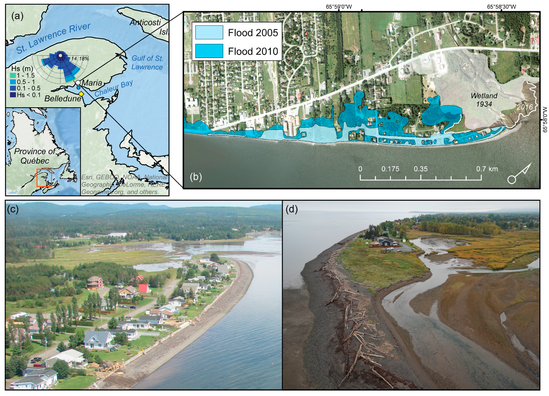
2.1. Study Area and Flood Surveys

The municipality of Maria in the Chaleur Bay (Québec, Canada) (Figure 1) suffered from two major flood events in December 2005 and December 2010. A large area was flooded during both events [20,21]. The study focuses on the most vulnerable area, an urbanized low-lying coast characterized by a beach terrace and the Pointe-Verte sand spit. The beach of Maria is composed of sand and gravel and the beachface is narrow, with an average width of ~22 m in the natural area and only 12 m in front of defense structures [22]. The defense structures were established mainly since the 90s and consist of small seawalls made of concrete and wood, and rock armor structures. They were mostly constructed on the upper beach to prevent erosion, with a structure toe above the higher average tide, and were not built to stand against high water levels and waves. The crest elevation is highly variable along the coastline, and overtopping occurs during extreme storms [20,21]. Cross-shore concrete boat ramps promote the accessibility to the beach, but also enhance overland flow in specific locations during storms. According to field observations, water flows inland during flood events [20], but does not return to sea: Flow routes are rather derived by roads and drainage systems through a salt marsh protected by the spit, but these processes have never been quantified.
Static flood mapping based on a fixed elevation threshold is particularly difficult in this area because inundation patterns are complex due to the proximity of the salt marsh at the back barrier of the spit (Figure 1c,d). Drainage was considered a critical source of flood mapping overprediction by Didier et al. [20], especially on the sandy low-lying area flooded both on 2 December 2005 and 6 December 2010 (Figure 1b). During 6 and 7 December 2010, a 2.2 km longshore field survey was carried out in Maria to locate the maximum floodwater levels, tracing storm debris lines using a RTK-GPS Thales ProMark3 system (x, y, z uncertainties of ±2 cm). One hundred eighty-eight (188) elevation points were used to recreate the landward limit of the 2010 flood (the larger flooded zone in blue in Figure 1b), and to extract the elevation values from a 2007 airborne LiDAR dataset (spatial resolution of 1 m, vertical accuracy of 20 cm) [20].

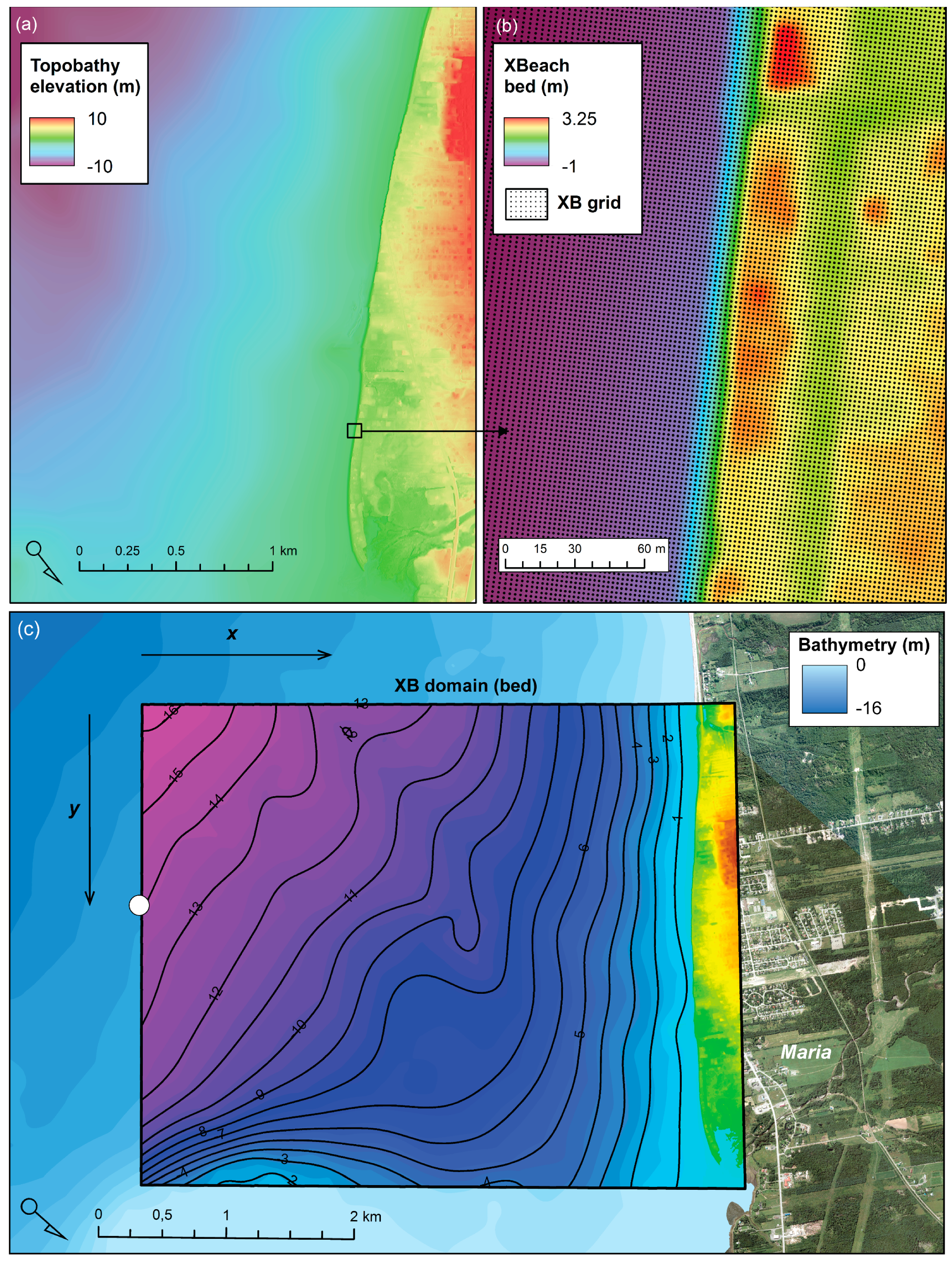
2.2. Topo-Bathymetric Data

High-resolution digital elevation models (DEMs) covering the entire flood simulation domains (offshore, nearshore, and inland topography) are needed for effective hazard assessments. In Maria, a seamless topo-bathymetric surface was created based on a combination of Mobile Terrestrial LiDAR surveys (MTLS) [20], airborne LiDAR, offshore bathymetry from the Canadian Hydrographic Service (CHS), and video-derived intertidal topography [73] (Figure 2a,b). The latter was used to recreate the elevation surface of the lower foreshore in front of one of the areas most prone to flooding. Furthermore, the intertidal topography in this area is complex due to the remnants of an old jetty (dismantled in 1945), which is unresolved with other acquisition techniques. The video-derived intertidal topography was created during the tidal cycle of 12 January 2016. The elevation matrix was generated with a 1 m × 1 m grid resolution (Figure 3a). We systematically refer to the Canadian Geodetic Vertical Datum 1928 (CGVD28) in this paper. The reader is referred to Appendix A for a detailed methodological description.

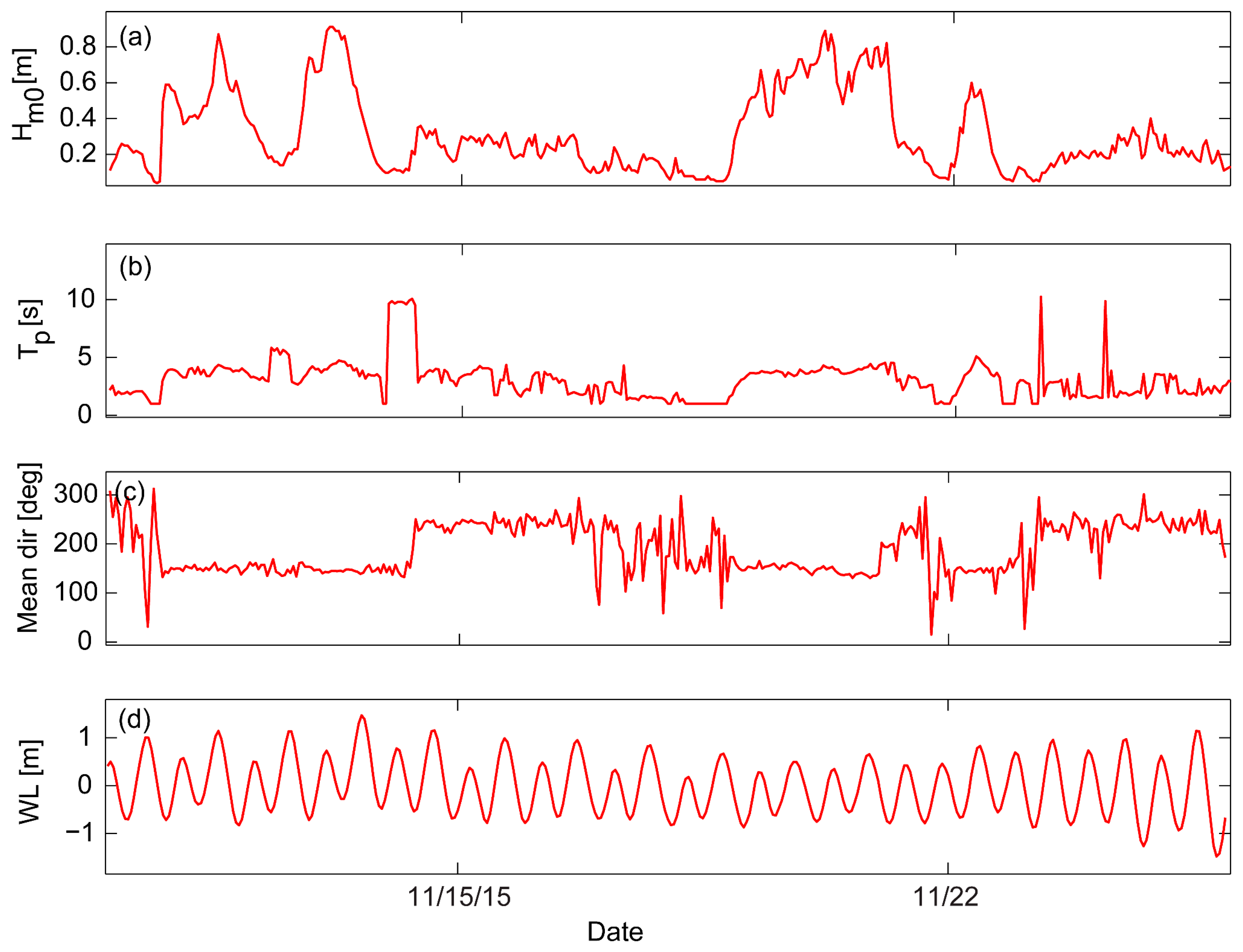
2.3. Offshore Waves and Water Levels

The beach of Maria is under the influence of a semi-diurnal and meso-tidal regime (tidal range < 3 m). The mean sea level (MSL) is located at 1.33 m relative to Chart Datum [74] (Table 1). During mid- and high-tides, the thin beach face is therefore mostly under water. For the boundary conditions in the 2010 flood simulations, hourly observed water levels (astronomical tide + storm surge) at the nearest tide gauge of Belledune (Canadian Hydrographic Service (CHS)) were used [75]. For the validation of XBeach, water levels were provided by a Nortek Acoustic Wave And Current profiler (AWAC) located offshore at 14 m deep (48.138000° N, −65.991997° W) (Figure 1a and Figure 3c).
The validation of XBeach was performed over a continuous survey period between 10–25 November 2015. The AWAC provided hourly observations of surface gravity waves and water levels during the entire survey (pressure at 1 Hz, AWAC-surface distance at 2 Hz). Statistical wave parameters include the spectral wave height (Hm0), mean period (T02), peak period (Tp), mean direction (θ), and directional spreading (s). Hourly wave boundary conditions for the 2010 flood simulation were extracted from WAVEWATCH III (see a description in Appendix A) with a 1 km grid resolution. The reader is referred to Didier et al. [33] and Bernatchez et al. [76] for a detailed explanation of the WW3 implementation in the EGSL. Based on the comparison between wave observations at the AWAC location and WW3 between 9–30 November 2015, Bernatchez et al. [76] observed a negative bias of −0.253 m (RMSE = 0.297 m) attributed to (1) the insufficient resolution of the CFSR wind forcing model in coastal environments and (2) bathymetric effects, which are not resolved in the 1 km grid simulations. This bias was statistically corrected on wave heights based on simple linear regressions following H0deb = H0/0.445 [76].

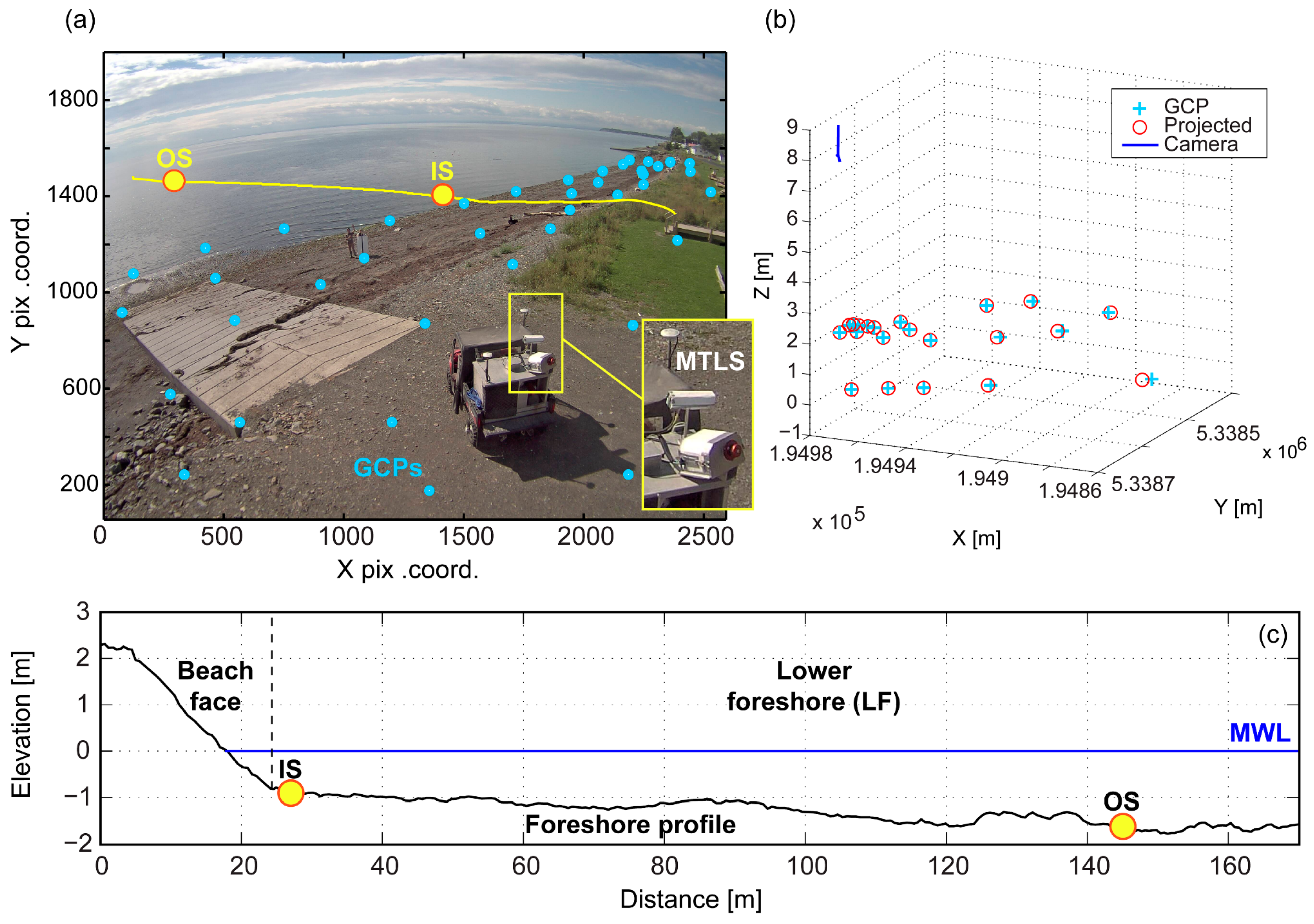
2.4. Nearshore Waves and XBeach Validation

Two pressure transducers (from RBR) were installed in the nearshore zone between 10–25 November 2015 to assess the performance of XBeach in simulating waves and water levels on the beach of Maria (Figure 2). One of them was bottom-mounted on the inner lower foreshore (IS), and the other on the outer lower foreshore (OS) (Figure 1 and Figure 2). Both instruments recorded continuous total pressure at 4 Hz. A spectral analysis was performed over a duration of 1024 s (17.06 min) to infer the significant wave height (Hs), mean period (Tm02), and mean water level (η). During the validation period, energetic events have been recorded in the area. Maximum offshore Hs reached 0.91 m (Tp = 4.5 s) on 13 November 2015 (Figure 4), which is considered as storm conditions in the Chaleur Bay [20]. Time-series of waves and water levels were coupled with the video-based shoreline detection to recreate the intertidal beach elevation. The location of both sensors in the camera view is shown in Figure 2a.
The coupled hydro- and -morphodynamic model, XBeach [66], was used to simulate the storm of December 2010 in Maria. The model simulates physical processes on various coastal environments, but was mainly built to predict storm impacts (e.g., swash, collision, overwash, and inundation [77]) on longshore-complex beaches [54]. XBeach solves the continuous water levels variations from short to long waves based on depth-averaged, non-linear shallow water equations. XBeach includes a hydrostatic (surfbeat) and a non-hydrostatic mode. For the purpose of this study, only the hydrodynamic module was implemented in 2D mode (2DH), and the morphological updating was turned off (morphology = 0). The 2DH model domain was created with a varying grid spacing, Δx, from 30 m at the offshore boundary to 2 m at the coast (Figure 3c). The longshore spacing, Δy, was fixed at 2 m. The domain covers an area of 19.34 km2 (5.05 km × 3.84 km). All the simulations were run in surfbeat mode, with the preserving wave groupiness option (single_dir = 1). Hourly wave characteristics (H0, Tp) from the AWAC were used to create parametric JONSWAP wave spectrums (shape, γ = 3.3, directional spreading of 20°). Front and back boundaries were set to absorbing-generating (weakly-reflective) in all simulations (front/back = abs_2d) (Van Dongeren and Svendsen 1997). Lateral boundaries were set to Neumann (left/right = neumann), imposing a longshore gradient of zero [78]. Other XBeach parameters were set to default.
The performance of XBeach in simulating the nearshore hydrodynamics and water levels was assessed with common statistical indicators. The mean bias errors (MBE) indicate the tendency of a model to over- or under-estimate, and was calculated following:
MBE = 1 n i = 1 n S i O i .
where Si and Oi are the simulation values and observations, respectively. The second model performance indicator is the root-mean-square error (RMSE):
RMSE = 1 n i = 1 n ( S i O i ) 2 .
Finally, the mean absolute error (MAE) is calculated
MAE = i = 1 n | S i O i | n .

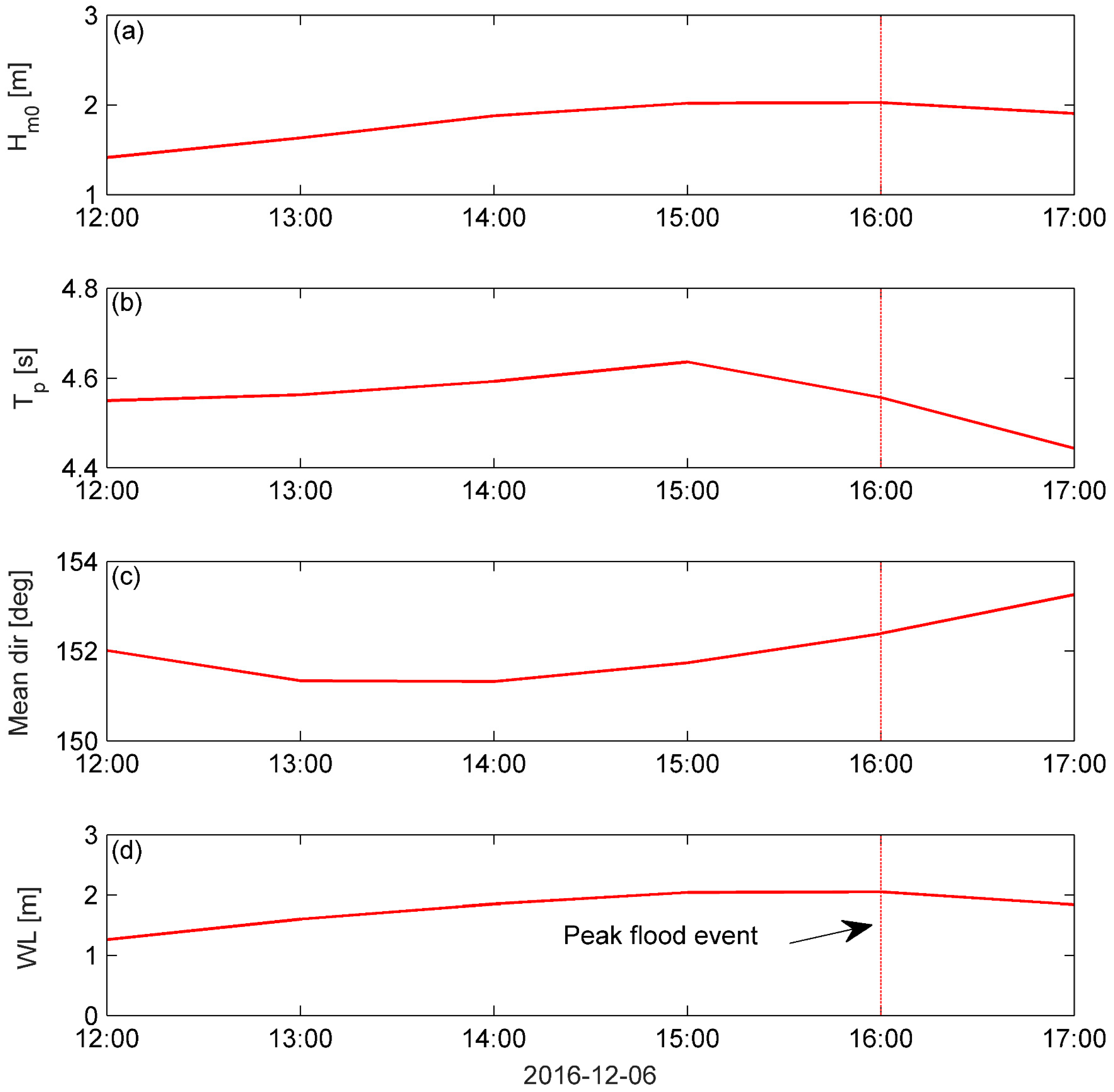
2.5. Actual and Future Design Storm Simulations

To assess the effect of rising sea levels in Maria in terms of identifying flood-prone areas, two storm scenarios were assessed through XBeach simulations using the same settings as in Section 2.4, but with an increase in sea level for the year of 2100. First, the storm event of 6 December 2010 was simulated with XBeach, with boundary conditions extracted from WW3 (same domain and grid as the validation) (Figure 5). According to Didier et al. [20], the flood occurred around 15–16 h (EST). Boundary conditions for the 6-hour long simulation are thus characterized by a high tide/surge of 2.05 m around 15–16 h (EST) (Figure 5d) occurring simultaneously with the highest waves of the joint event (Hm0 = 2.03 m) (Figure 5a).
A hypothetical storm scenario for the year of 2100 was simulated based on an increase in sea level only, assuming a stable future wave climate. The observed rate of sea level rise is both the result of eustatic sea level variations and regional glacio-isostatic adjustments (GIA) along Atlantic Canada [5,42,43,44], varying between −1 and −4 mm/year in the Gulf of St Lawrence [5,45]. The relative sea level has risen at a mean rate of 0.93 ± 1.25 mm/ year over the past ~1500 years in the Chaleur Bay and GIA was a significant contributor to this rate [79]. In recent decades, sea level rise has increased at a mean rate of 4.06 mm/year at the Belledune tide gauge between 1964–2014 (Figure 1a). In the absence of sea level rise projections for the study area, we applied this constant rate to obtain a hypothetical scenario for 2100, which is considered sufficient to assess the influence of sea level rise on flood propagation patterns. Sea level rise was applied to the water level time-series between 2010–2100, resulting in a peak water level boundary condition of ~2.42 m in 2100. For both flood simulations, outputs were generated at 10-min intervals.

3. Results and Discussion

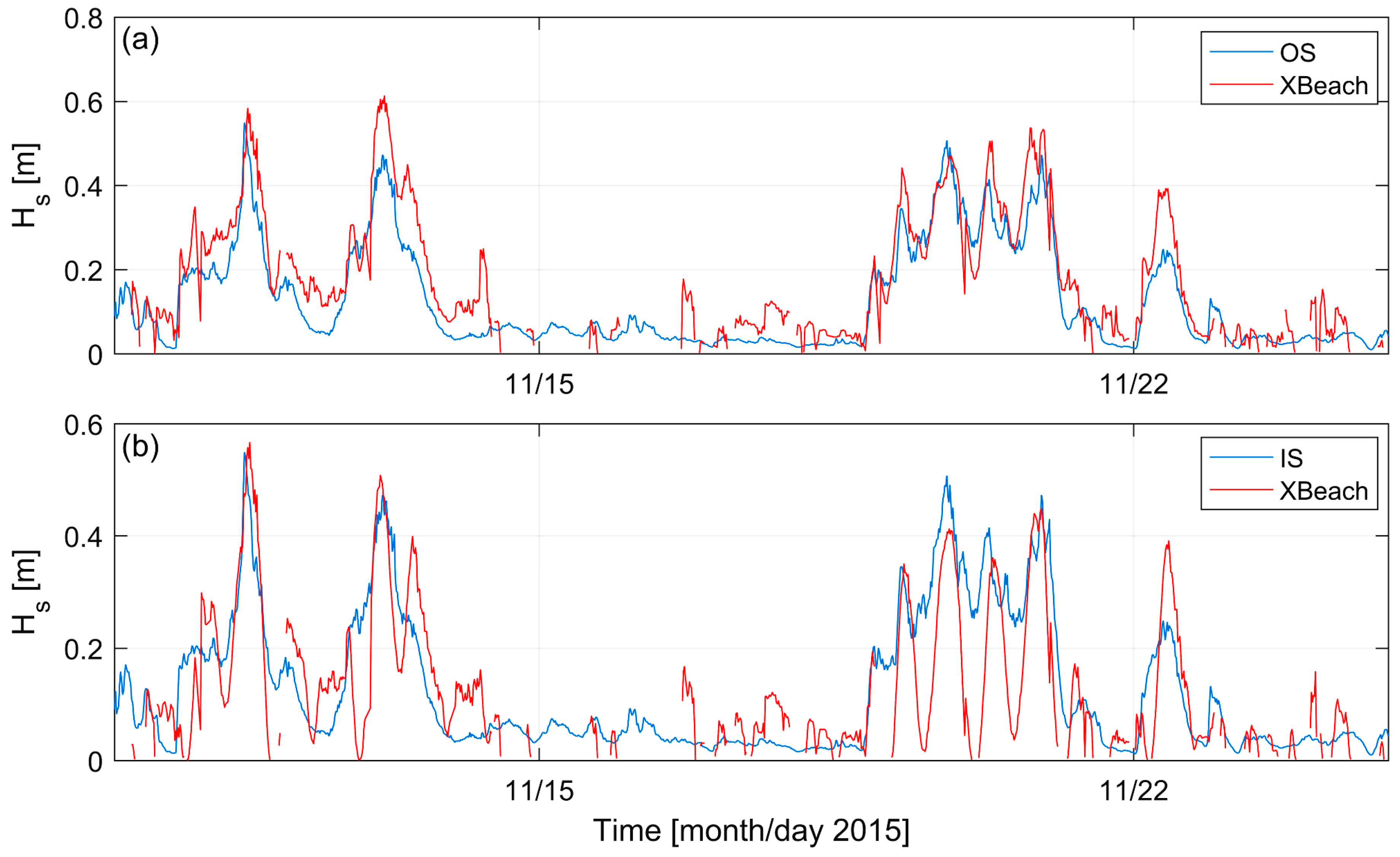
3.1. XBeach Validation

Validation results for the parameter, Hs, indicate a good prediction of the XBeach 2DH model compared to observations in the nearshore zone on both sensors (ρ2 > 0.8) (Table 2). All performance indicators are under 0.07 cm, which is consistent with other studies (e.g., [33,71]). Overall, there is no tendency to over- or under-estimate wave heights in the nearshore zone (MBE close to 1 on both sensors) and regression lines have a nearly null intercept (a2 = ±0.01). Some underpredictions are nevertheless observed near the coastline (IS between 19 and 21 November 2015) (Figure 6b), mostly under low-energy conditions with small waves (Hs < 20cm), which appears to be due to water level oscillations. Since most underpredictions seem to occur during low tides while short waves would break and dissipate their energy across the lower foreshore, we assume this should not affect the results of the flood simulations during the peak event. Validation results for the mean water level (not included in Table 2) are virtually within a centimeter-scale deviation from the observations (r2 = 0.99).

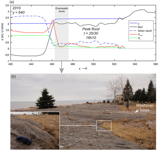
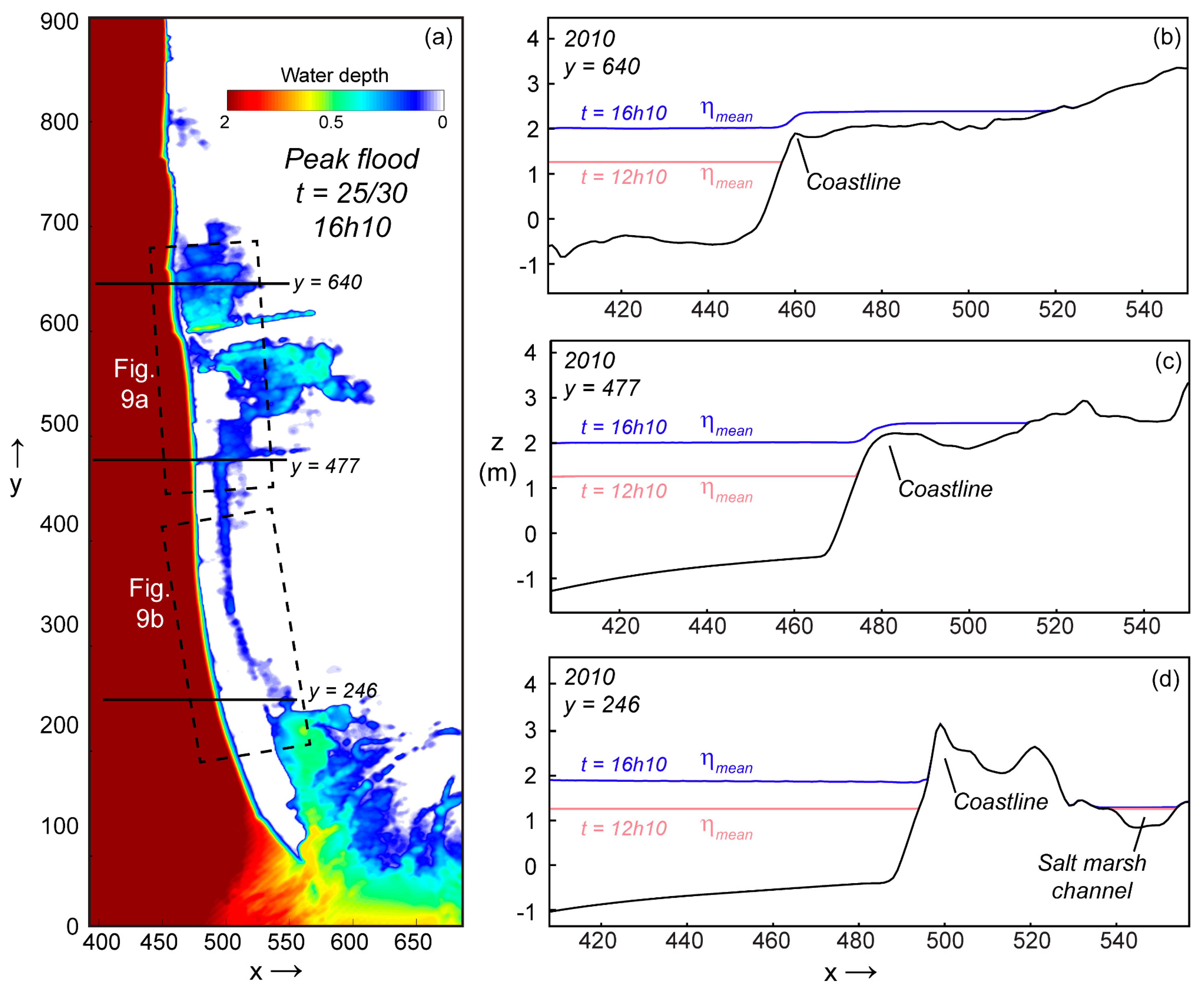
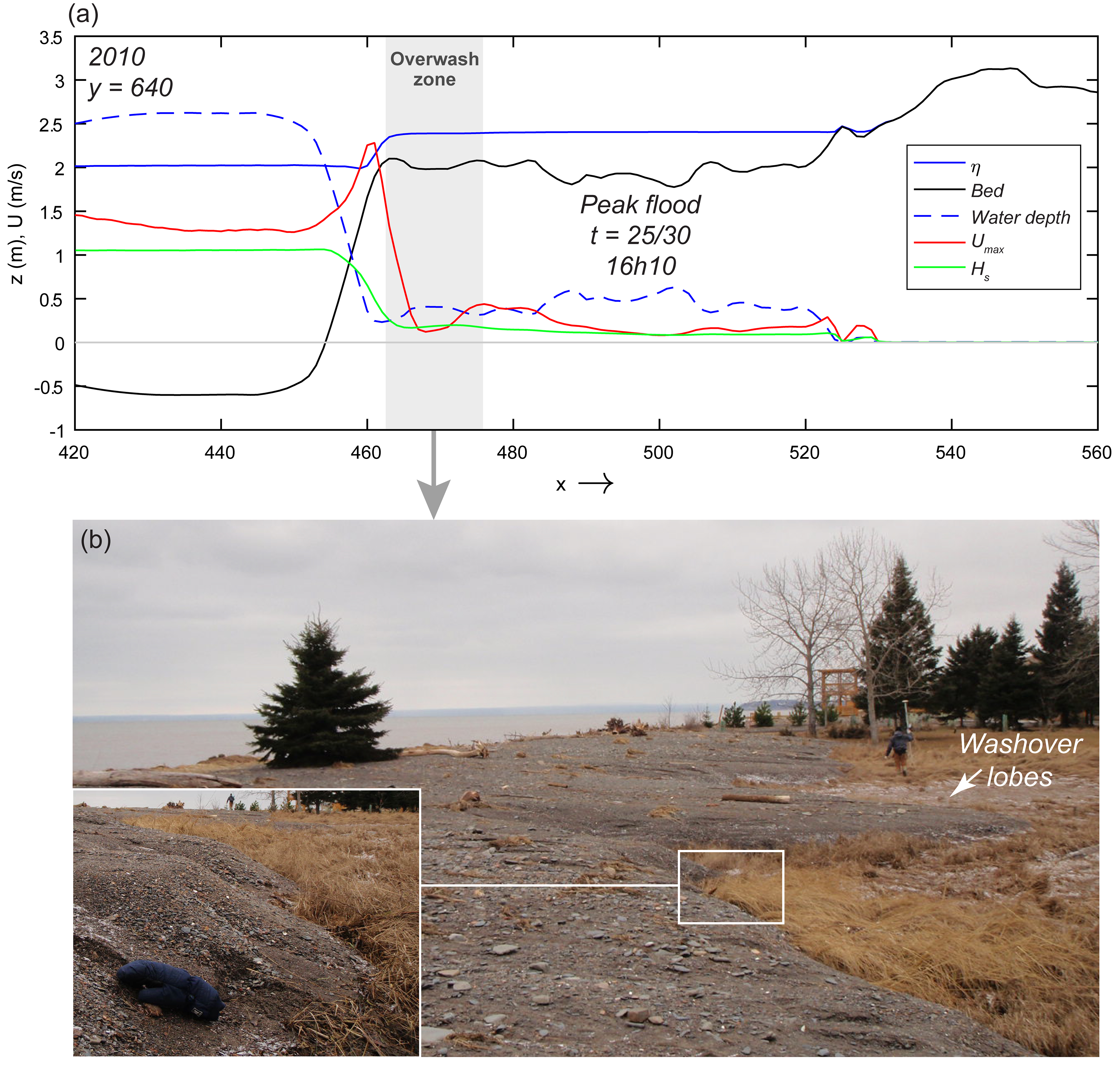
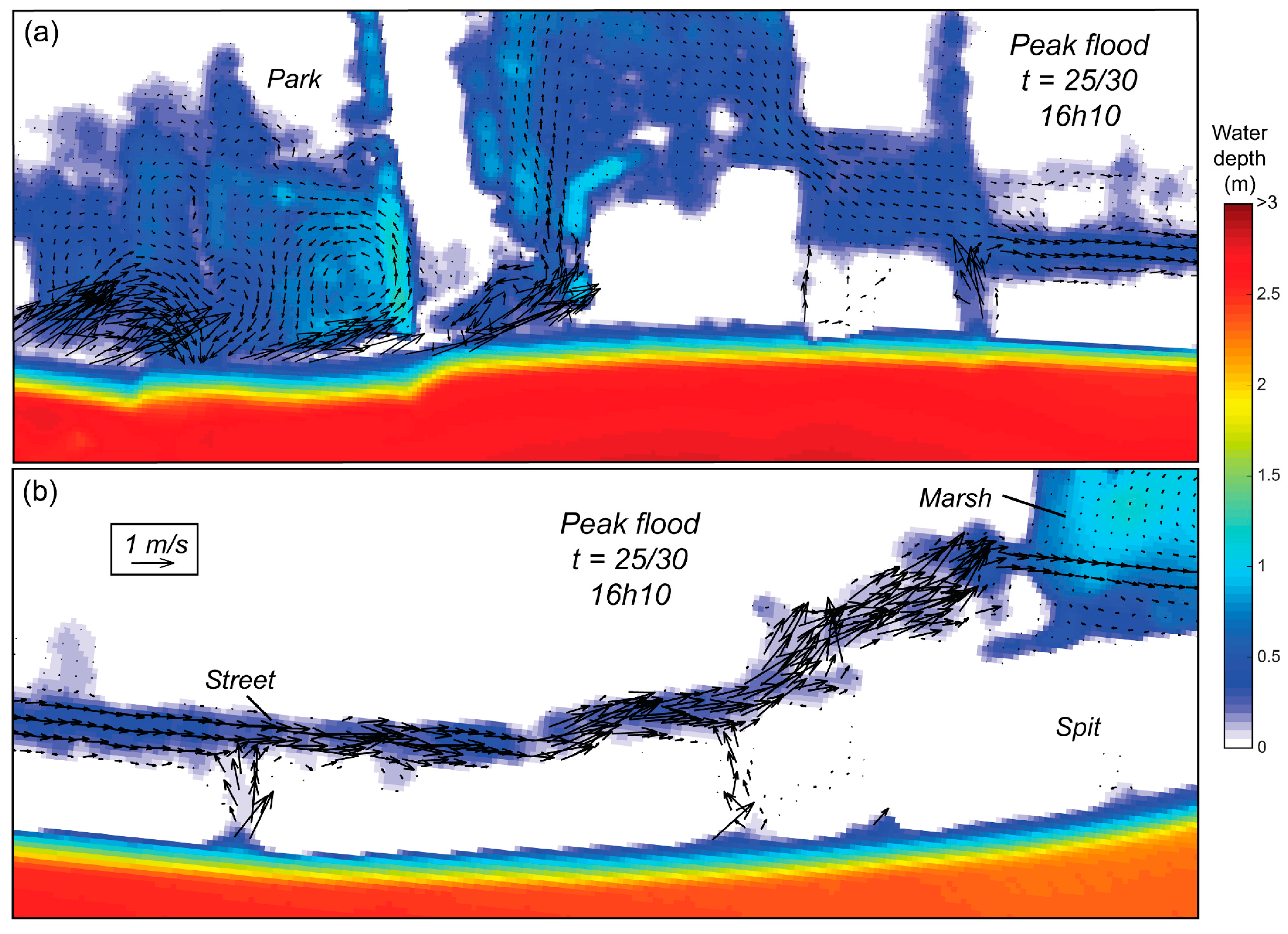
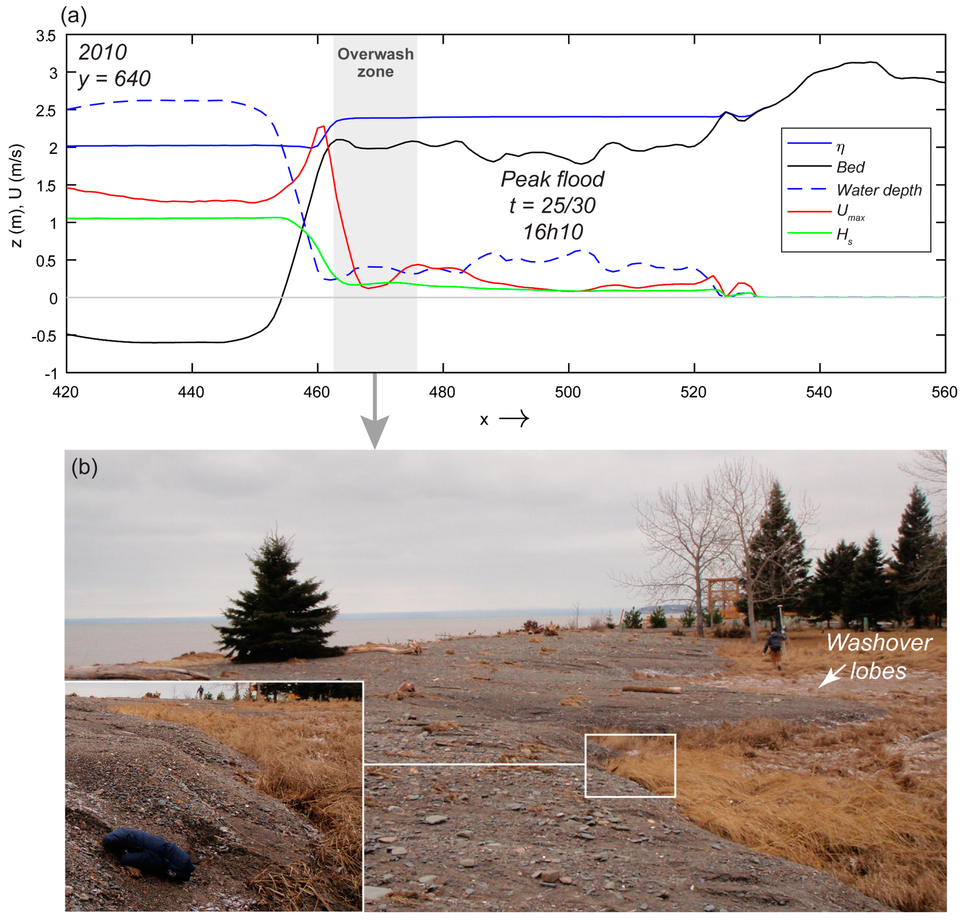
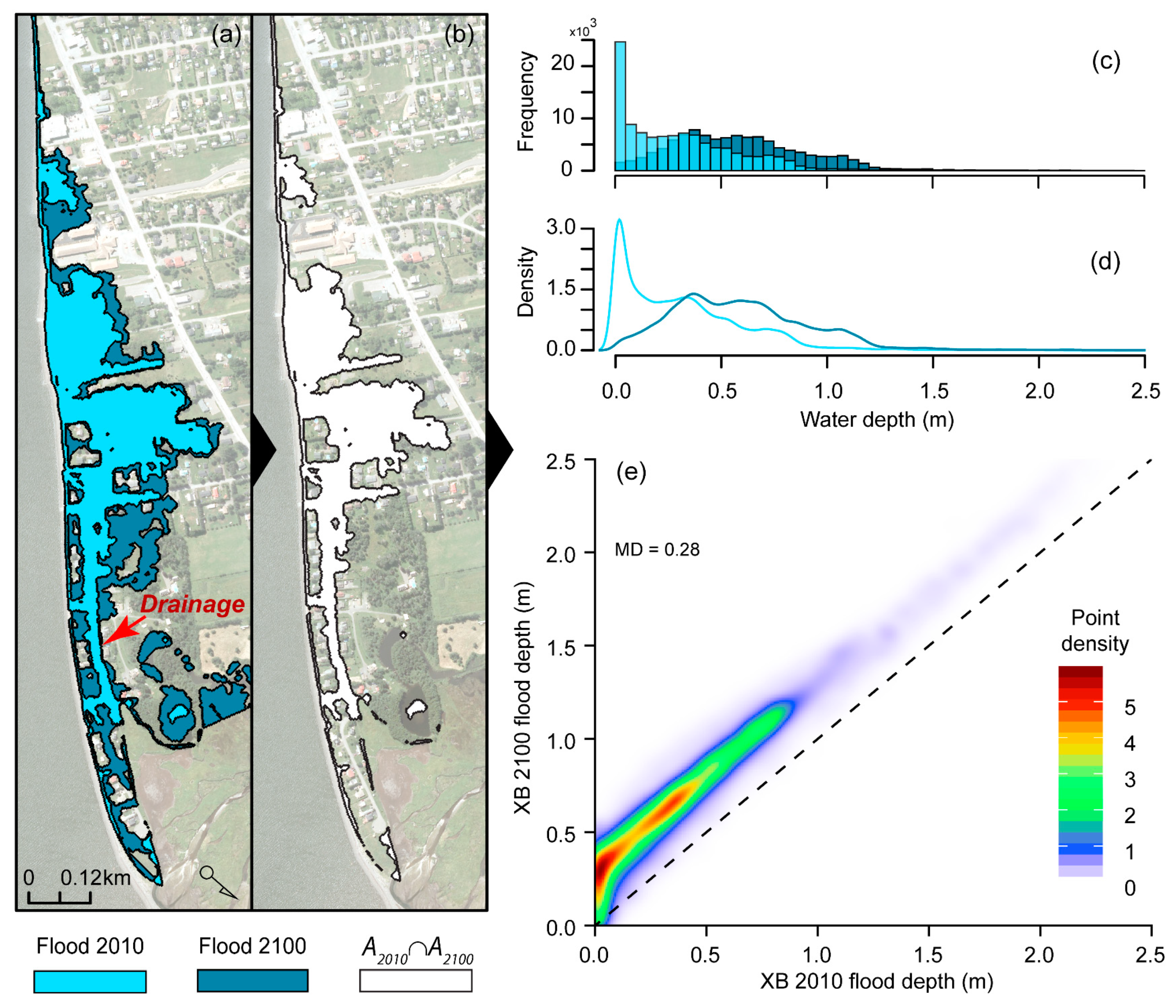
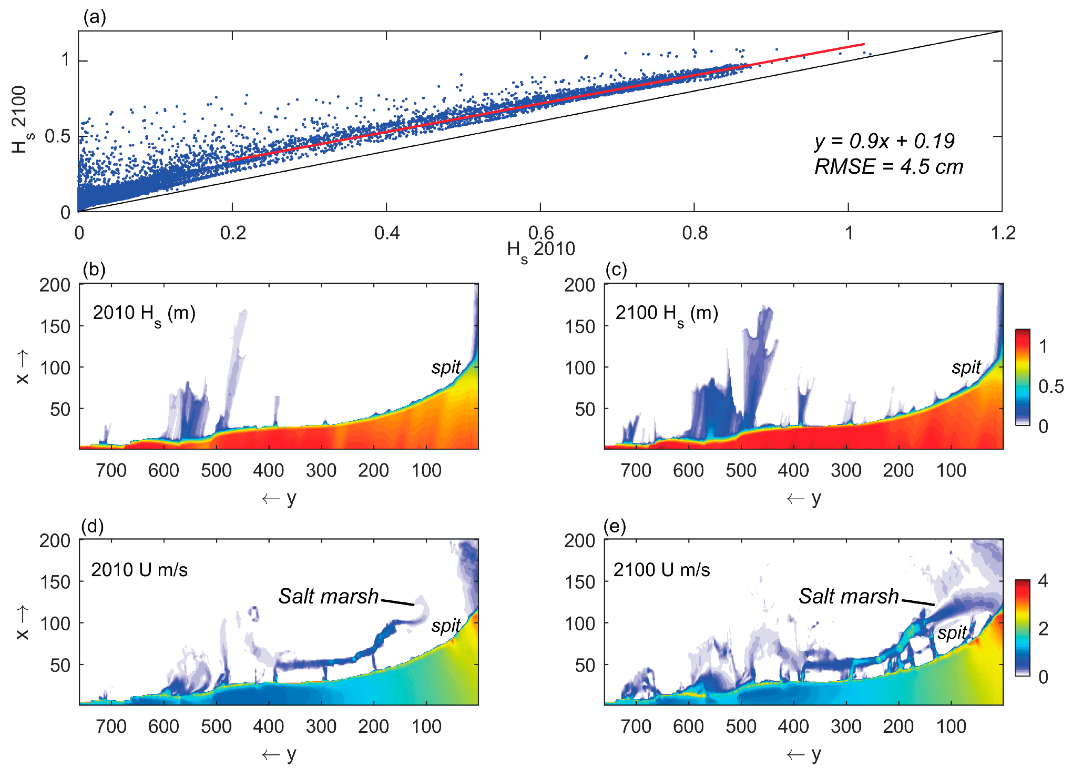
3.2. Understanding the Flood Propagation

During the storm of 6 December 2010, high water levels reached the sandy-gravel beach of Maria and flooded the urbanized low-lying spit and surrounding area (Figure 7a). The performance of XBeach was assessed by comparing the predicted flooded area with field observations (RTK-GPS) on 6 and 7 December 2010 (see Section 2.1). The coefficient of aerial correspondence (critical success or fit (F)) [80], defined as the area both flooded and correctly predicted as flooded by the model, was calculated following:
F = A o b s A p r e d A o b s A p r e d ,
where F is the ratio of the intersection and union of observed (Aobs = 0.151 km2, considering only the inland area without the salt marsh) and predicted (Apred) floods (0.099 km2) (Figure 7a). According to Equation (5), the overall fit of the 2DH simulation for the 2010 event is 59%.
The model results indicate that flooding was globally induced by overwash and surge-driven flow landward of the coastline (Figure 8). Furthermore, flow channels developed on boat access and ramps perpendicular to the coastline, acting as artificial breaches for flow propagation (Figure 8, e.g., y = 477). Inland flows were essentially concentrated in the streets and lateral drainage systems, directing the gravity-driven surface waters toward the salt marsh [20]. Apart from being located at a lower elevation, the marsh acted as a buffer zone for water level fluctuations. This is visible in Figure 8d, where the water level at the most landward boundary of the salt marsh, at the back of the spit, is the same at t = 12 h 10 and t = 16 h 10. The 2DH model clearly captures the essential drainage process in dampening the inland flood propagation, as seen in Figure 9, from the flow direction.
The flood propagation essentially covered the low-lying area of the park and adjacent urbanized areas along the main street. Flow velocities were mostly less than 0.5 m/s (Figure 9), and flood depths systematically less than 1 m. The most important flow velocities are observed near the coastline, with a maximum velocity around ~2.5 m/s in the main overwashing entrance (Figure 9a).
The use of XBeach as a 2D coastal inundation model is still developing. Its validation is typically done with field measurements of simulated water levels and waves. To assess the impact of sea level rise on small islands with XBeach (calibrated and without morphological updating), Quataert et al. [71] validated the simulated hydrodynamic parameters in the nearshore zone with field measurements in Roi-Namur (Marshall Islands). They obtained good agreement with observations. More recently, van Dongeren et al [72] presented flood simulations for the same island and noted that some overwash were not simulated by the model. Elsayed and Oumeraci [32] demonstrated the effectiveness of XBeach in simulating the combined effect of breaching and inundation. Their case study applied to a real dam breach (Het Zwin [66]) showed good agreement with water depth and flow velocities virtually at any given point in the hinterland, despite slight overestimations of velocities in the order of 6–15%. Although the morphodynamic module was not implemented in the Maria case, the results of the hydrodynamic simulations against the observed flood extents also demonstrate that XBeach in 2DH mode offers good performances. The fit ratio (F) of ~60% is well within the performances of other models obtained in flood simulations. For instance, in a pan-European study using LISFLOOD-FP, fits between 43–65% were observed by Alfieri et al. [81]. With the same model, Bates et al. [82] and Vousdoukas et al. [25] respectively obtained F values of the order of 54–91% and 49%. Recently, using XBeach in surfbeat mode, Didier et al. [33] simulated the extreme flood of 6 December 2010 in the St. Lawrence Maritime Estuary, and obtained an averaged critical success of 51% over nine different domains. XBeach therefore offers a successful alternative to common hydrological models, such as LISFLOOD-FP and BreZo, for coastal flood assessment, with the advantage of simulating nearshore dynamics, including low frequency wave motions, which are generally important during storms on low-sloping nearshore environment, such as Maria [71]. Furthermore, the 2DH mode provides the flow routes of the flood event, which is often an important source of confusion in flood simulation based on static water levels [50].
In the present study, XBeach enhanced the understanding of storm impacts on the coast of Maria and contributed to a better understanding of the flood hazard not only in terms of static flood surface (spatial extent), but also in a more dynamic sense considering the timing, intensity, and duration of the event affecting the flow-related processes and the water depth. These are critical parameters in disaster risk management [83,84].
The storm impact scale from Sallenger [77] defines the overwash regime as a situation when wave runup is higher than the first line of defense (i.e., coastline), which creates net landward sediment transport and accumulation. Such morphodynamic response is only possible when water depth and flow velocity are sufficient [85]. Typically, overwash is the result of flow velocities of 1–3.5 m/s and water depths of at least 0.7 m [77,86]. During the RTK-GPS surveys in December 2010, photographs taken on the field near the XBeach grid point [x = 460, y = 640] (see Figure 10a,b) clearly show the net landward sediment transport resulting from overwash processes. Washover lobes (Figure 10b) formed under a mean water depth of ~0.5–0.6 m and maximum flow velocities, Umax, varying between 2.28 m/s near the shoreline prior to overwashing. On the beach crest, velocities reached 1.34 m/s (Figure 10a). Velocities rapidly decrease with the flow distance inland to ~0.3–0.4 m/s. Wave height does not exceed 1 m on the beach face along the cross-shore profile and decreases to 0.2 m on the beach crest, suggesting the overwash is mainly due to the surge-driven flow landwards of the coastline. Another way to improve our understanding of the morphodynamics during this event would be to run XBeach with morphological updating, which introduces sediments fluxes, avalanching, and bed characteristics [78]. XBeach was previously used to represent overtopping and overflow hydrodynamics (e.g., [32,50,87]). However, Phillips et al. [53] suggest that neglecting the morphological impacts may significantly underestimate overtopping volumes. Morphological updating would imply many more calibration steps and require more quantitative information on evolving topo-bathymetry [69] that would go beyond the scope of this paper. Furthermore, the lack of pre/post-storm sediment characteristics could greatly impact the model result [88].

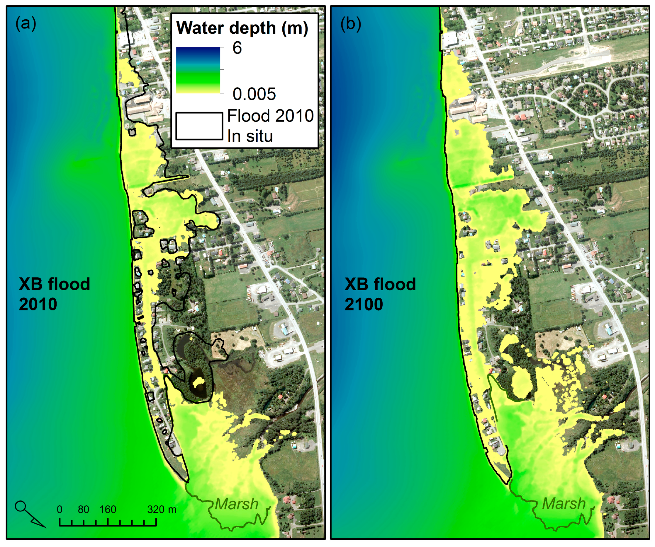
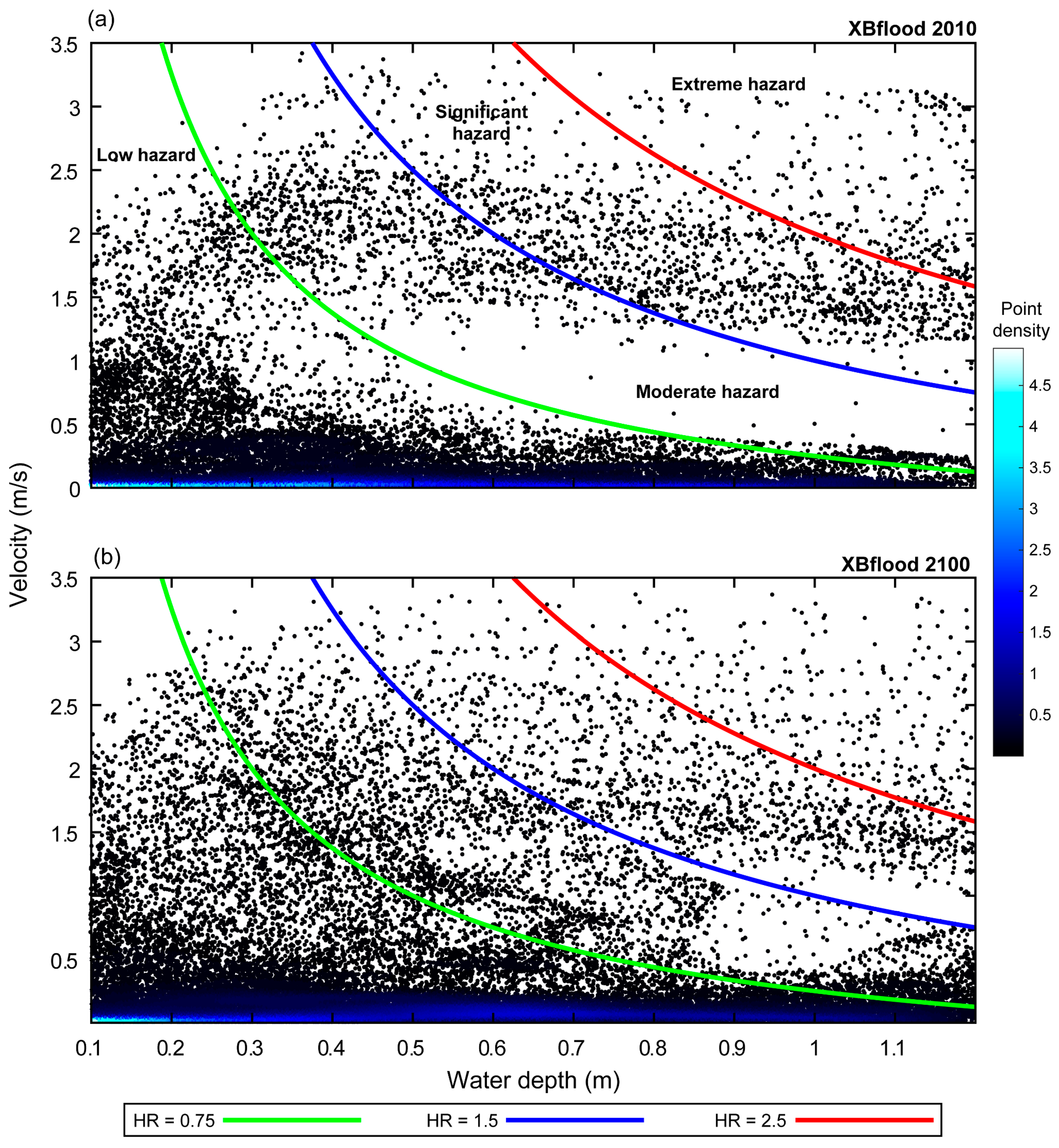
3.3. Impacts of Sea Level Rise on Flood Hazard

Based on the same hydrodynamic boundary conditions as the simulation of the 6 December 2010 storm event in Maria, an increase in sea level up to 2100 (peak event at 2.05 in 2010 compared to 2.42 in 2100) would induce an increase in 178% of the flood zone area (0.176 km2 in 2100 compared to 0.099 km2 in 2010) (Figure 11a). The totality of the area flooded in 2010 is also simulated as flooded in 2100 (see A 2010 A 2100 in Figure 11b), but the flood in 2100 is essentially larger due to higher water levels. Average flood depth is almost doubled in 2100 (an average depth of 59.4 cm in 2100 compared to 31.5 cm in 2010) (Figure 11c,d). This is mainly the result of a major shift in flood depths from the very shallow waters (i.e., <25 cm where the peak density is observed) to slightly deeper values between 0.5 and 1.25 m (Figure 11c,d). However, the topography is a key parameter to consider in flood mapping since drainage can drastically reduce flood extents [42], even for future flood scenarios, as seen on Figure 11a, where both the 2010 and 2100 simulations have the same flooded area along the main street (as shown by the red arrow). Considering the flood propagation for coastal flood mapping is therefore crucial for effective hazard assessments in a context of changing climate, and numerical simulations provide such possibilities over static flood mapping.
Flood risk management (e.g., flood mapping) and coastal engineering projects (e.g., establishing design standards) are commonly based on design storm scenarios representing extreme events with a long return period (RP) (i.e., often a 100-year RP, or an annual probability of occurring of 0.01) [89,90]. In Canada, the probability of exceeding a specific storm intensity within a certain period of time is commonly associated to a static intensity-duration-frequency (IDF) curve for a given hazard (e.g., river flooding, coastal flooding), without considering climate change [91]. In coastal areas, this often means neglecting the effect of climate variability on nearshore dynamics, such as wave runup and wave climate [19,92].
Coastal communities along the Estuary and Gulf of St. Lawrence are highly vulnerable to coastal hazards [37,93,94]. Impacts of sea level rise on nearshore dynamics and flood propagation have never been assessed, yet stakeholders and land-planners recently ranked the roads as the most highly vulnerable infrastructure to flooding in the Chaleur Bay [37]. In Maria, the XBeach simulations clearly demonstrate an effect of higher water levels both on wave height (Figure 12a–c) and velocity (Figure 12d,e), impacting not only the coast, but also the local roads. For a given grid location affected by floodwater in 2010, Hs are approximately 19 cm higher in 2100 compared to 2010 (considering only Hs > 0.2 to avoid uncertainties for small waves) (r2 = 0.93, p-value < 0.01) (Figure 12a). This small increase is the result of higher overwash and overtopping volumes over the coastline under higher wave energy in the nearshore zone. Once inland, the flow in the 2100 simulation has higher velocities (U > 2 m/s in 2100, point grid [y = 180, x = 90]), and literally follow the main street toward the salt marsh with a continuous flow (Figure 12e) compared to 2010 where the flow was ~1.2 m/s before abruptly dropping to almost zero in the salt marsh (Figure 12d).
Global-scale coastal flood assessments are commonly made with a static approach of simulated total water levels [95], without considering critical physical processes (e.g., groundwater fluctuations, sediment porosity, channeling and land drainage, wave runup, and overtopping, etc.) affecting the flood propagation. At the regional scale, this kind of basic flood mapping is often needed by stakeholders and land-planners as a first-order approximation of potential extreme hazard [96], but their uncertainties generally limit their reliability for future assessment. Despite significant advances in sea-level projections at local and regional scales [62,64], simulations for the Québec coasts are rather rare.
In Maria, our results suggest that the actual trend in sea level, extrapolated up to 2100, which is a scenario that can be considered optimistic, could potentially induce a massive urban flood twice as large as the extreme storm of December 2010, for an event of the same magnitude. However, unlike static and raster-based flood modelling, the process-based model, XBeach, simulates a dynamic flood zone in Maria, and thus a better understanding of the flood pattern, including the effect of drainage and morphology. Despite being site-specific to the Maria case, these results suggest that other low-lying communities along the EGSL where urbanization took place on late-Holocene emerged beach terrace (i.e., relatively plane surface) could suffer from sea level rise. That could trigger important risk not only to human settlements [97], but also directly to people and emergency services during peak floods. As seen in Figure 13, sea level rise can potentially increase the risk to people by increasing not only the water depth for a given design storm scenario, but also by shifting the flooded area toward higher velocity flows and therefore more danger to people [98]. For instance, Ramsbottom et al. [98] suggested an empirical formulation relating flood hazard to people (HR, m2/s) to water depth (d) and velocities (v) following:
HR = d ( v + 0.5 ) + D F
where 0.5 is a velocity coefficient and DF a debris factor of 0, 0.5, or 1.
Assuming no debris, we can estimate the effect of sea level rise on HR within four typical hazard classes: low hazard (HR < 0.75), moderate hazard (0.75 < HR < 1.5), significant hazard (1.5 < HR < 2.5), and extreme hazards (HR > 2.5) (Figure 13). Based on these thresholds, not only the flood zone will be larger in Maria with sea level rise, but it will also slightly increase the hazard to people during a peak flood event, such as the 6 December 2010 storm (Figure 13b).
According to this classification, extreme and significant hazards are essentially rare in Maria, corresponding respectively to 1% and 2–3% of the flood zone in the 2010 and 2100 simulations, respectively. Although most observations (93% in 2010, 90% in 2100) fall under the low hazard level (HR < 0.75), sea level rise induces a small shift toward higher danger, doubling the moderate hazard frequency to 7% in 2100 compared to 3.5% in 2010. Such statistics improve the understanding of the extreme flood and offer a coastal management perspective that helps to better define evacuation routes for timely evacuation and effective early warning [99,100]. It should be noted that such hazard thresholds are based on the stability of people in water: For instance, some people (i.e., children) are assumed to be greatly affected by a moderate hazard, while most people could be affected by the significant hazard [34].

4. Conclusions

This paper presented a coastal flood analysis with XBeach, implemented at a local scale for a small urban community in the Chaleur Bay, eastern Canada. The 6 December 2010 historical flood in Maria was well predicted with the 2DH model in surfbeat mode. According to the numerical simulation, flooding was mainly induced by overwashing along the beach, which was also supported with field observations. Observations of sediment accumulations in the form of washover lobes in Maria are associated to velocities of 2.3 m/s under small waves (e.g., Hs < 1 m) and high water levels. The flood propagated toward the salt marsh following the topographic gradient, which underlines the importance of land drainage for coastal flood adaptation strategies.
Consequences of sea level rise on coastal communities are generally uncertain due to many factors inherent to flood modelling, especially the effect of overland flow (e.g., namely water depth, velocities, pathways). Using a sea level rise scenario for 2100 to force XBeach, which more precisely means a rise of 0.37 m in Maria, the same storm would increase the extent of the flooded area as a result of higher water levels, more overwash, and overflow along the coastline. Sea level rise increases the water depth in the flood prone area. Nearshore waves are slightly increased, generating higher flow velocity along the main channels and streets. This study underlines the necessity to account for the inland processes during coastal flood assessment, as a better understanding of the overland flow routing leads to improved flood mitigation strategies for future storm and sea level rise scenarios. In this context, it becomes necessary to develop local-scale relative sea level rise projections in eastern Canada that integrate new developments in climate and GIA models.

Author Contributions

This research was conceptualized by D.D. (David Didier) and P.B.; it was written by D.D. (David Didier) under the supervision of P.B. and D.D. (Dany Dumont). Numerical modelling and data analysis was performed by D.D. (David Didier) and M.B.

Funding

This study was funded by the Coastal Geoscience Chair at the Université du Québec at Rimouski as part of the Québec Government initiative on natural risks prevention and the Plan d’action 2013–2020 sur les changements climatiques et du Fonds Vert.

Acknowledgments

The authors want to acknowledge the works of Jeremy Baudry and James Caveen during the simulations. Special thanks to Christian Fraser and Tarik Toubal for the field surveys during the 2010 storm and to the LDGIZC hydrodynamic team in 2015, namely Denys Dubuc, Gabriel Montpetit and Pierre-André Lalanne. The video-monitoring station was implemented with the help of Emmanuel Augereau from LGO, Brest, France.

Conflicts of Interest

The authors declare no conflict of interest. The funders had no role in the design of the study; in the collection, analyses, or interpretation of data; in the writing of the manuscript, or in the decision to publish the results.

Abbreviations

DEMDigital Elevation Model
DFDebris Factor
DTMDigital Terrain Model
DSMDigital Surface Model
EGSLEstuary and Gulf of St. Lawrence
GCPGround Control Points
GIAGlacio-Isostatic Adjustment
HATHighest Astronomical Tide
HRHazard Rating
IDFIntensity-Duration-Frequency
ISInner lower foreshore sensor
LATLowest Astronomical Tide
MTLSMobile Terrestrial LiDAR Survey
OSOuter lower foreshore sensor
RTK-GPSReal-Time Kinematic Global Navigation Satellite System
RPReturn Period
SWLStill water level
TWLTotal Water Level

Appendix A

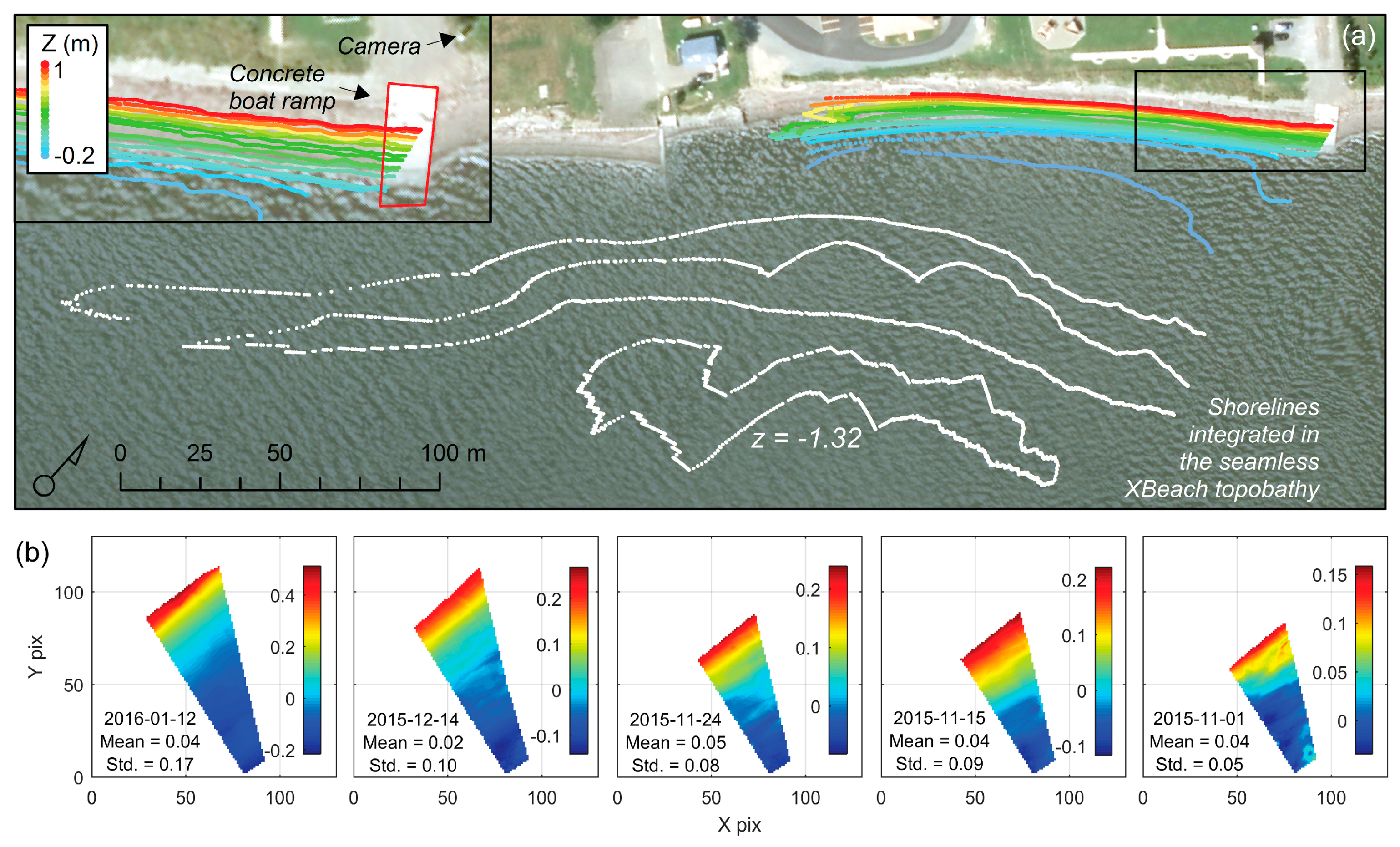
Appendix A.1. Video-Derived Intertidal Topobathymetry

To recreate a digital elevation model of the intertidal zone in front of Maria, a video monitoring system (AXIS P3367VE, 4 Hz, 2592 × 1944 pixels, 5 megapixels, pan range of 84°) was used in combination with a shoreline detection technique based on color ratios between the beach sediments and the water [73,101]. This water/land junction, known as the shoreline, is systematically extracted in pixel coordinates from successive 5-min time-averaged video-images (1200 images) during a tidal cycle in calm conditions (Hs < 15 cm). To include the effect of waves on shoreline locations, the total water level (TWL) was given by the summation of the mean water level and Hs at the outer sensor. The resulting shoreline is attributed the same TWL elevation and projected into ground coordinates according to a conversion matrix based on Grounds Control Points (GCPs) (Figure 2a,b) [102]. The last step involves merging the entire shoreline datasets into a single elevation matrix with an ANUDEM interpolation technique [103].
Figure A1. Validation of the video-derived beach topography on the concrete boat ramp for five different experiments on the beach of Maria, including the survey of January 2016, which is integrated into the seamless topobathy for the XBeach simulations. Colorbars indicate the shoreline elevations (a) and the deviation Δ Video-MTLS (b).
Geosciences 09 00076 g0a1
To assess the effectiveness of this method, we compared five interpolated surfaces created from five different video surveys to the MTLS elevation. The MTLS was conducted in October 2015 to acquire beach topography, including a concrete boat ramp built on the beach. The LiDAR cloudpoint (resolution of 5 cm × 5 cm, RMSE = 0.03) was filtered manually using LP360 to remove wood debris. The concrete slab was used as a target for the validation of the video-derived topography (Figure A1). Overall, the mean deviation of the video-derived topography is systematically under 5 cm for all surveys. This positive bias is mostly affected by the detected shorelines at high tide around a small spatial area (between the rising/falling tide) and should not influence the performance of the video-derived DEM at low tide. For the topobathymetric surface, only the shorelines on the lower foreshore on 12 January 2016 were integrated into the seamless elevation model. The MTLS covers the entire upper beach along the study area.

Appendix A.2. Description of the WW3 Hindcast

To produce the wave and water level boundary conditions for the 2010 storm event, the third-generation model WW3 version 4.18 [104] was used to recreate the wave climate in the EGSL at a 1km-grid resolution. This version integrates both the attenuation of incident wave energy by sea ice through scattering and the viscous dissipation, giving a more realistic representation of the effect of wave-ice interactions over the wave field during winter. Oceanic forcings in the EGSL wave model (currents, water levels, sea ice) were provided by a coastal ice-ocean model forced by the NCEP North American Regional Reanalysis (NARR) and the atmospheric forcing comes from the Climate Forecast System Reanalysis (CFSR).

References

  1. Luijendijk, A.; Hagenaars, G.; Ranasinghe, R.; Baart, F.; Donchyts, G.; Aarninkhof, S. The State of the World’s Beaches. Sci. Rep. 2018, 1–11. [Google Scholar] [CrossRef] [PubMed]
  2. Muis, S.; Verlaan, M.; Nicholls, R.J.; Brown, S.; Hinkel, J.; Lincke, D.; Vafeidis, A.T.; Scussolini, P.; Winsemius, H.C.; Ward, P.J. A comparison of two global datasets of extreme sea levels and resulting flood exposure. Earth Future 2017, 5, 379–392. [Google Scholar] [CrossRef]
  3. Wahl, T.; Haigh, I.D.; Nicholls, R.J.; Arns, A.; Dangendorf, S.; Hinkel, J.; Slangen, A.B.A. Understanding extreme sea levels for broad-scale coastal impact and adaptation analysis. Nat. Commun. 2017, 8, 1–12. [Google Scholar] [CrossRef] [PubMed]
  4. Hinkel, J.; Lincke, D.; Vafeidis, A.T.; Perrette, M.; Nicholls, R.J.; Tol, R.S.J.; Marzeion, B.; Fettweis, X.; Ionescu, C.; Levermann, A. Coastal flood damage and adaptation costs under 21st century sea-level rise. Proc. Natl. Acad. Sci. USA 2014, 111, 3292–3297. [Google Scholar] [CrossRef] [PubMed]
  5. Koohzare, A.; Vaníček, P.; Santos, M. Pattern of recent vertical crustal movements in Canada. J. Geodyn. 2008, 45, 133–145. [Google Scholar] [CrossRef]
  6. Ruest, B.; Neumeier, U.; Dumont, D.; Bismuth, E.; Senneville, S.; Caveen, J. Recent wave climate and expected future changes in the seasonally ice-infested waters of the Gulf of St. Lawrence, Canada. Clim. Dyn. 2016, 46, 449–466. [Google Scholar] [CrossRef]
  7. Lerma, A.N.; Bulteau, T.; Elineau, S.; Paris, F.; Durand, P.; Anselme, B.; Pedreros, R. High-resolution marine flood modelling coupling overflow and overtopping processes: Framing the hazard based on historical and statistical approaches. Nat. Hazards Earth Syst. Sci. 2018, 18, 207–229. [Google Scholar] [CrossRef]
  8. Tomás, A.; Méndez, F.J.; Medina, R.; Jaime, F.F.; Higuera, P.; Lara, J.L.; Ortiz, M.D.; Álvarez de Eulate, M.F. A methodology to estimate wave-induced coastal flooding hazard maps in Spain. J. Flood Risk Manag. 2016, 9, 289–305. [Google Scholar] [CrossRef]
  9. Hawkes, P.J.; Gouldby, B.P.; Tawn, J.A.; Owen, M.W. The joint probability of waves and water levels in coastal engineering design. J. Hydraul. Res. 2002, 40, 241–251. [Google Scholar] [CrossRef]
  10. Prime, T.; Brown, J.M.; Plater, A.J. Flood inundation uncertainty: The case of a 0.5% annual probability flood event. Environ. Sci. Policy 2016, 59, 1–9. [Google Scholar] [CrossRef]
  11. Melet, A.; Meyssignac, B.; Almar, R.; Le Cozannet, G. Under-estimated wave contribution to coastal sea-level rise. Nat. Clim. Chang. 2018, 8, 234–239. [Google Scholar] [CrossRef]
  12. Moftakhari, H.R.; AghaKouchak, A.; Sanders, B.F.; Matthew, R.A. Cumulative hazard: The case of nuisance flooding. Earth Future 2017, 5, 214–223. [Google Scholar] [CrossRef]
  13. Sadegh, M.; Moftakhari, H.; Gupta, H.V.; Ragno, E.; Mazdiyasni, O.; Sanders, B.; Matthew, R.; AghaKouchak, A. Multihazard Scenarios for Analysis of Compound Extreme Events. Geophys. Res. Lett. 2018, 45, 5470–5480. [Google Scholar] [CrossRef]
  14. Vitousek, S.; Barnard, P.L.; Fletcher, C.H.; Frazer, N.; Erikson, L.; Storlazzi, C.D. Doubling of coastal flooding frequency within decades due to sea-level rise. Sci. Rep. 2017, 7, 1399. [Google Scholar] [CrossRef]
  15. Viavattene, C.; Jiménez, J.A.; Ferreira, O.; Priest, S.; Owen, D.; McCall, R. Selecting coastal hotspots to storm impacts at the regional scale: A Coastal Risk Assessment Framework. Coast. Eng. 2018, 134, 33–47. [Google Scholar] [CrossRef]
  16. Pollard, J.A.; Spencer, T.; Brooks, S.M. The interactive relationship between coastal erosion and flood risk. Prog. Phys. Geogr. 2018. [Google Scholar] [CrossRef]
  17. Colle, B.A.; Booth, J.F.; Chang, E.K.M. A Review of Historical and Future Changes of Extratropical Cyclones and Associated Impacts Along the US East Coast. Curr. Clim. Chang. Rep. 2015, 125–143. [Google Scholar] [CrossRef]
  18. Bernatchez, P. Implantation d’un réseau de suivi de l’érosion côtière et bilan de l’érosion pour le Bas-Saint-Laurent, la Gaspésie et les Îles-de-la-Madeleine, Québec. Rapport remis au Ministère des Affaires municipales et des régions du Québec; Ministère des Affaires municipales et des régions du Québec: Rimouski, QC, Canada, 2006.
  19. Didier, D.; Bernatchez, P.; Marie, G.; Boucher-Brossard, G. Wave runup estimations on platform-beaches for coastal flood hazard assessment. Nat. Hazards 2016. [Google Scholar] [CrossRef]
  20. Didier, D.; Bernatchez, P.; Boucher-Brossard, G.; Lambert, A.; Fraser, C.; Barnett, R.; Van-Wierts, S. Coastal Flood Assessment Based on Field Debris Measurements and Wave Runup Empirical Model. J. Mar. Sci. Eng. 2015, 3, 560–590. [Google Scholar] [CrossRef]
  21. Bernatchez, P.; Fraser, C.; Lefaivre, D.; Dugas, S. Integrating anthropogenic factors, geomorphological indicators and local knowledge in the analysis of coastal flooding and erosion hazards. Ocean Coast. Manag. 2011, 54, 621–632. [Google Scholar] [CrossRef]
  22. Daigle, R.J. Sea Level Rise Estimates for New Brunswick Municipalities: Saint John, Sackville, Richibucto, Shippagan, Caraquet, Le Goulet; A Report for the Atlantic Climate Adaptation Solutions Association; Atlantic Climate Adaptation Solutions Association: New Brunswick, NB, Canada, 2011.
  23. Quintin, C.; Bernatchez, P.; Jolivet, Y. Impacts de la tempête du 6 décembre 2010 sur les côtes du Bas-Saint-Laurent et de la baie des Chaleurs; Rapport d’analyse: Volume I; Présenté au ministère de la Sécurité publique du Québec: Rimouski, QC, USA, 2013; Volume I.
  24. Harley, M. Coastal Storm Definition. In Coastal Storms; John Wiley & Sons, Ltd.: Chichester, UK, 2017; pp. 1–21. ISBN 9781118937105. [Google Scholar]
  25. Vousdoukas, M.I.; Voukouvalas, E.; Mentaschi, L.; Dottori, F.; Giardino, A.; Bouziotas, D.; Bianchi, A.; Salamon, P.; Feyen, L. Developments in large-scale coastal flood hazard mapping. Nat. Hazards Earth Syst. Sci. 2016, 16, 1841–1853. [Google Scholar] [CrossRef]
  26. Breilh, J.F.; Chaumillon, E.; Bertin, X.; Gravelle, M. Assessment of static flood modeling techniques: Application to contrasting marshes flooded during Xynthia (western France). Nat. Hazards Earth Syst. Sci. 2013, 13, 1595–1612. [Google Scholar] [CrossRef]
  27. Orton, P.; Vinogradov, S.; Georgas, N.; Blumberg, A.; Lin, N.; Gornitz, V.; Little, C.; Jacob, K.; Horton, R. New York City Panel on Climate Change 2015 Report Chapter 4: Dynamic Coastal Flood Modeling. Ann. N. Y. Acad. Sci. 2015, 1336, 56–66. [Google Scholar] [CrossRef] [PubMed]
  28. Patrick, L.; Solecki, W.; Jacob, K.H.; Kunreuther, H.; Nordenson, G. New York City Panel on Climate Change 2015 Report Chapter 3: Static Coastal Flood Mapping. Ann. N. Y. Acad. Sci. 2015, 1336, 45–55. [Google Scholar] [CrossRef] [PubMed]
  29. Poulter, B.; Halpin, P.N. Raster modelling of coastal flooding from sea-level rise. Int. J. Geogr. Inf. Sci. 2008, 22, 167–182. [Google Scholar] [CrossRef]
  30. Van de Sande, B.; Lansen, J.; Hoyng, C. Sensitivity of Coastal Flood Risk Assessments to Digital Elevation Models. Water 2012, 4, 568–579. [Google Scholar] [CrossRef]
  31. Ramirez, J.A.; Lichter, M.; Coulthard, T.J.; Skinner, C. Hyper-resolution mapping of regional storm surge and tide flooding: Comparison of static and dynamic models. Nat. Hazards 2016, 82, 571–590. [Google Scholar] [CrossRef]
  32. Elsayed, S.; Oumeraci, H. Combined Modelling of Coastal Barrier Breaching and Induced Flood Propagation Using XBeach. Hydrology 2016, 3, 32. [Google Scholar] [CrossRef]
  33. Didier, D.; Baudry, J.; Bernatchez, P.; Dumont, D.; Sadegh, M.; Bismuth, E.; Bandet, M.; Dugas, S.; Sévigny, C. Multihazard simulation for coastal flood mapping: Bathtub versus numerical modelling in an open estuary, Eastern Canada. J. Flood Risk Manag. 2018, e12505. [Google Scholar] [CrossRef]
  34. Kvočka, D.; Falconer, R.A.; Bray, M. Flood hazard assessment for extreme flood events. Nat. Hazards 2016, 84, 1569–1599. [Google Scholar] [CrossRef]
  35. Kumar, V.S.; Babu, V.R.; Babu, M.T.; Dhinakaran, G.; Rajamanickam, G.V. Assessment of Storm Surge Disaster Potential for the Andaman Islands. J. Coast. Res. 2008, 24, 171–177. [Google Scholar] [CrossRef]
  36. Kim, K.; Pant, P.; Yamashita, E. Integrating travel demand modeling and flood hazard risk analysis for evacuation and sheltering. Int. J. Disaster Risk Reduct. 2018, 31, 1177–1186. [Google Scholar] [CrossRef]
  37. Fraser, C.; Bernatchez, P.; Dugas, S. Development of a GIS coastal land-use planning tool for coastal erosion adaptation based on the exposure of buildings and infrastructure to coastal erosion, Québec, Canada. Geomat. Nat. Hazards Risk 2017, 8, 1103–1125. [Google Scholar] [CrossRef]
  38. Webster, T.L. Flood Risk Mapping Using LiDAR for Annapolis Royal, Nova Scotia, Canada. Remote Sens. 2010, 2, 2060–2082. [Google Scholar] [CrossRef]
  39. Guimarães, P.V.; Farina, L.; Toldo, E.; Diaz-Hernandez, G.; Akhmatskaya, E. Numerical simulation of extreme wave runup during storm events in Tramandaí Beach, Rio Grande do Sul, Brazil. Coast. Eng. 2015, 95, 171–180. [Google Scholar] [CrossRef]
  40. Sayol, J.M.; Marcos, M. Assessing Flood Risk Under Sea Level Rise and Extreme Sea Levels Scenarios: Application to the Ebro Delta (Spain). J. Geophys. Res. Ocean. 2018, 123, 794–811. [Google Scholar] [CrossRef]
  41. Brown, J.D.; Spencer, T.; Moeller, I. Modeling storm surge flooding of an urban area with particular reference to modeling uncertainties: A case study of Canvey Island, United Kingdom. Water Resour. Res. 2007, 43, 1–22. [Google Scholar] [CrossRef]
  42. Gallien, T.W.; Sanders, B.F.; Flick, R.E. Urban coastal flood prediction: Integrating wave overtopping, flood defenses and drainage. Coast. Eng. 2014, 91, 18–28. [Google Scholar] [CrossRef]
  43. Leon, J.X.; Phinn, S.R.; Hamylton, S.; Saunders, M.I. Filling the “white ribbon”—A multisource seamless digital elevation model for Lizard Island, northern Great Barrier Reef. Int. J. Remote Sens. 2013, 34, 6337–6354. [Google Scholar] [CrossRef]
  44. Le Roy, S.; Pedreros, R.; André, C.; Paris, F.; Lecacheux, S.; Marche, F.; Vinchon, C. Coastal flooding of urban areas by overtopping: Dynamic modelling application to the Johanna storm (2008) in Gâvres (France). Nat. Hazards Earth Syst. Sci. 2015, 15, 2497–2510. [Google Scholar] [CrossRef]
  45. Gallien, T.; Kalligeris, N.; Delisle, M.-P.; Tang, B.-X.; Lucey, J.; Winters, M. Coastal Flood Modeling Challenges in Defended Urban Backshores. Geosciences 2018, 8, 450. [Google Scholar] [CrossRef]
  46. Narayan, S.; Simmonds, D.; Nicholls, R.J.; Clarke, D. A Bayesian network model for assessments of coastal inundation pathways and probabilities. J. Flood Risk Manag. 2018, 11, S233–S250. [Google Scholar] [CrossRef]
  47. Bernatchez, P.; Fraser, C. Evolution of Coastal Defence Structures and Consequences for Beach Width Trends, Québec, Canada. J. Coast. Res. 2012, 285, 1550–1566. [Google Scholar] [CrossRef]
  48. Pullen, T.; Allsop, N.W.H.; Bruce, T.; Kirtenhaus, A.; Schüttrumpf, H.; van der Meer, J.W. Eurotop: Wave Overtopping of Sea Defences and Related Structures: Assessment Manual; Kuratorium für Forschung im Küsteningenieurwesen (KFKI)—Die Küste: Hamburg, Germany, 2007. [Google Scholar]
  49. Van der Meer, J.W.; Allsop, N.W.H.; Bruce, T.; De Rouck, J.; Kortenhaus, A.; Pullen, T.; Schüttrumpf, H.; Troch, P.; Zanuttigh, B. Manual on Wave Overtopping of Sea Defences and Related Structures. An Overtopping Manual Largely Based on European Research, but for Worldwide Application. 2016. Available online: www.overtopping-manual.com (accessed on 30 January 2019).
  50. Gallien, T.W. Validated coastal flood modeling at Imperial Beach, California: Comparing total water level, empirical and numerical overtopping methodologies. Coast. Eng. 2016, 111, 95–104. [Google Scholar] [CrossRef]
  51. Chini, N.; Stansby, P.K. Extreme values of coastal wave overtopping accounting for climate change and sea level rise. Coast. Eng. 2012, 65, 27–37. [Google Scholar] [CrossRef]
  52. Tsoukala, V.K.; Chondros, M.; Kapelonis, Z.G.; Martzikos, N.; Lykou, A.; Belibassakis, K.; Makropoulos, C. An integrated wave modelling framework for extreme and rare events for climate change in coastal areas—The case of Rethymno, Crete. Oceanologia 2016, 58, 71–89. [Google Scholar] [CrossRef]
  53. Phillips, B.; Brown, J.; Bidlot, J.-R.; Plater, A. Role of Beach Morphology in Wave Overtopping Hazard Assessment. J. Mar. Sci. Eng. 2017, 5, 1. [Google Scholar] [CrossRef]
  54. Roelvink, D.; McCall, R.; Mehvar, S.; Nederhoff, K.; Dastgheib, A. Improving predictions of swash dynamics in XBeach: The role of groupiness and incident-band runup. Coast. Eng. 2018, 134, 103–123. [Google Scholar] [CrossRef]
  55. Cohn, N.; Ruggiero, P. The influence of seasonal to interannual nearshore profile variability on extreme water levels: Modeling wave runup on dissipative beaches. Coast. Eng. 2015, 115, 79–92. [Google Scholar] [CrossRef]
  56. Leijala, U.; Björkqvist, J.-V.; Johansson, M.M.; Pellikka, H.; Laakso, L.; Kahma, K.K. Combining probability distributions of sea level variations and wave run-up to evaluate coastal flooding risks. Nat. Hazards Earth Syst. Sci. Discuss. 2018, 1–25. [Google Scholar] [CrossRef]
  57. Li, N.; Yamazaki, Y.; Roeber, V.; Cheung, K.F.; Chock, G. Probabilistic mapping of storm-induced coastal inundation for climate change adaptation. Coast. Eng. 2018, 133, 126–141. [Google Scholar] [CrossRef]
  58. Bates, P.; De Roo, A.P. A simple raster-based model for flood inundation simulation. J. Hydrol. 2000, 236, 54–77. [Google Scholar] [CrossRef]
  59. Bates, P.D.; Horritt, M.S.; Fewtrell, T.J. A simple inertial formulation of the shallow water equations for efficient two-dimensional flood inundation modelling. J. Hydrol. 2010, 387, 33–45. [Google Scholar] [CrossRef]
  60. Begnudelli, L.; Sanders, B.F.; Bradford, S.F. Adaptive Godunov-Based Model for Flood Simulation. J. Hydraul. Eng. 2008, 134, 714–725. [Google Scholar] [CrossRef]
  61. Roelvink, J.A.; Van Banning, G.K.F.M. Design and development of DELFT3D and application to coastal morphodynamics. Oceanogr. Lit. Rev. 1995, 42, 925–938. [Google Scholar]
  62. Kopp, R.E.; Horton, R.M.; Little, C.M.; Mitrovica, J.X.; Oppenheimer, M.; Rasmussen, D.J.; Strauss, B.H.; Tebaldi, C. Probabilistic 21st and 22nd century sea-level projections at a global network of tide-gauge sites. Earth Future 2014, 2, 383–406. [Google Scholar] [CrossRef]
  63. Goodwin, P.; Haigh, I.D.; Rohling, E.J.; Slangen, A. A new approach to projecting 21st century sea-level changes and extremes. Earth Future 2017, 5, 240–253. [Google Scholar] [CrossRef]
  64. Meyssignac, B.; Fettweis, X.; Chevrier, R.; Spada, G. Regional Sea Level Changes for the Twentieth and the Twenty-First Centuries Induced by the Regional Variability in Greenland Ice Sheet Surface Mass Loss. J. Clim. 2017, 30, 2011–2028. [Google Scholar] [CrossRef]
  65. Purvis, M.J.; Bates, P.D.; Hayes, C.M. A probabilistic methodology to estimate future coastal flood risk due to sea level rise. Coast. Eng. 2008, 55, 1062–1073. [Google Scholar] [CrossRef]
  66. Roelvink, D.; Reniers, A.; Van Dongeren, A.; Van Thiel De Vries, J.; Mccall, R.; Lescinski, J. Modelling storm impacts on beaches, dunes and barrier islands. 2009, 56, 1133–1152. [Google Scholar] [CrossRef]
  67. Poelhekke, L.; Jäger, W.S.; van Dongeren, A.; Plomaritis, T.A.; McCall, R.; Ferreira, Ó. Predicting coastal hazards for sandy coasts with a Bayesian Network. Coast. Eng. 2016, 118, 21–34. [Google Scholar] [CrossRef]
  68. Barnard, P.L.; van Ormondt, M.; Erikson, L.H.; Eshleman, J.; Hapke, C.; Ruggiero, P.; Adams, P.N.; Foxgrover, A.C. Development of the Coastal Storm Modeling System (CoSMoS) for predicting the impact of storms on high-energy, active-margin coasts. Nat. Hazards 2014, 74, 1095–1125. [Google Scholar] [CrossRef]
  69. Simmons, J.A.; Harley, M.D.; Marshall, L.A.; Turner, I.L.; Splinter, K.D.; Cox, R.J. Calibrating and assessing uncertainty in coastal numerical models. Coast. Eng. 2017, 125, 28–41. [Google Scholar] [CrossRef]
  70. De Santiago, I.; Morichon, D.; Abadie, S.; Reniers, A.J.H.M.; Liria, P. A comparative study of models to predict storm impact on beaches. Nat. Hazards 2017, 87, 843–865. [Google Scholar] [CrossRef]
  71. Quataert, E.; Storlazzi, C.; Van Rooijen, A.; Cheriton, O.; Van Dongeren, A. The influence of coral reefs and climate change on wave-driven flooding of tropical coastlines. Geophys. Res. Lett. 2015, 42, 6407–6415. [Google Scholar] [CrossRef]
  72. Van Dongeren, A.R.; Storlazzi, C.D.; Quataert, E.; Pearson, S. Wave Dynamics and Flooding on Low-Lying Tropical Reef-Lined Coasts. Coast. Dyn. 2017, 2017, 654–664. [Google Scholar]
  73. Didier, D.; Bernatchez, P.; Augereau, E.; Caulet, C.; Dumont, D.; Bismuth, E.; Cormier, L.; Floc’h, F.; Delacourt, C. LiDAR Validation of a Video-Derived Beachface Topography on a Tidal Flat. Remote Sens. 2017, 9, 826. [Google Scholar] [CrossRef]
  74. Xu, Z.; Lefaivre, D. Prévision des niveaux d’ eau dans l’ estuaire et le golfe du Saint-Laurent en fonction des changements climatiques; Rapport interne au Ministère des Transports du Québec; Ministère des Transports du Québec: Montreal, QC, Canada, 2015.
  75. CHS Canadian Tides and Water Levels data Archives. Available online: http://www.isdm-gdsi.gc.ca/isdm-gdsi/twl-mne/index-eng.htm (accessed on 20 March 2015).
  76. Bernatchez, P.; Arsenault, E.; Lambert, A.; Bismuth, E.; Didier, D.; Senneville, S.; Dumont, D. Programme de mesure et de modélisation de la morphodynamique de l’érosion et de la submersion côtière dans l’estuaire et le golfe du Saint-Laurent (MODESCO), Phase II: Rapport Final; Université du Québec à Rimouski: Rimouski, QC, Canada, 2017. [Google Scholar]
  77. Sallenger, A.H. Storm impact scale for barrier islands. J. Coast. Res. 2000, 16, 890–895. [Google Scholar]
  78. Roelvink, D.; van Dongeren, A.; McCall, R.; Hoonhout, B.; van Rooijen, A.; van Geer, P.; de Vet, L.; Nederhoff, K.; Quataert, E. XBeach Technical Reference: Kingsday Release. Model Description and Reference Guide to Functionalities; Technical Report; Deltares: Delft, The Netherlands, 2015. [Google Scholar]
  79. Barnett, R.L.; Bernatchez, P.; Garneau, M.; Brain, M.J.; Charman, D.J.; Stephenson, D.B.; Haley, S.; Sanderson, N. Late Holocene sea-level changes in eastern Québec and potential drivers. Quat. Sci. Rev. 2019, 203, 151–169. [Google Scholar] [CrossRef]
  80. Taylor, P.J. Quantitative Methods in Geography: An Introduction to Spatial Analysis; Houghton Mifflin Harcourt: Boston, MA, USA, 1977. [Google Scholar]
  81. Alfieri, L.; Salamon, P.; Bianchi, A.; Neal, J.; Bates, P.; Feyen, L. Advances in pan-European flood hazard mapping. Hydrol. Process. 2014, 28, 4067–4077. [Google Scholar] [CrossRef]
  82. Bates, P.D.; Dawson, R.J.; Hall, J.W.; Horritt, M.S.; Nicholls, R.J.; Wicks, J.; Hassan, M.A.A.M. Simplified two-dimensional numerical modelling of coastal flooding and example applications. Coast. Eng. 2005, 52, 793–810. [Google Scholar] [CrossRef]
  83. Zheng, F.; Leonard, M.; Westra, S. Application of the design variable method to estimate coastal flood risk. J. Flood Risk Manag. 2017, 10, 522–534. [Google Scholar] [CrossRef]
  84. Didier, D.; Bernatchez, P.; Dumont, D. Systèmes d’alerte précoce pour les aléas naturels et environnementaux: Virage ou mirage technologique? Rev. Sci. l’eau 2017, 30, 115. [Google Scholar] [CrossRef]
  85. Matias, A.; Williams, J.J.; Masselink, G.; Ferreira, Ó. Overwash threshold for gravel barriers. Coast. Eng. 2012, 63, 48–61. [Google Scholar] [CrossRef]
  86. Matias, A.; Masselink, G. Overwash Processes: Lessons from Fieldwork and Laboratory Experiments. In Coastal Storms; John Wiley & Sons, Ltd.: Chichester, UK, 2017; pp. 175–194. [Google Scholar]
  87. Christie, E.K.; Spencer, T.; Owen, D.; McIvor, A.L.; Möller, I.; Viavattene, C. Regional coastal flood risk assessment for a tidally dominant, natural coastal setting: North Norfolk, southern North Sea. Coast. Eng. 2017, 1–14. [Google Scholar] [CrossRef]
  88. McCall, R.T.; Masselink, G.; Poate, T.G.; Roelvink, J.A.; Almeida, L.P.; Davidson, M.; Russell, P.E. Modelling storm hydrodynamics on gravel beaches with XBeach-G. Coast. Eng. 2014, 91, 231–250. [Google Scholar] [CrossRef]
  89. Ruggiero, P.; Hacker, S.; Seabloom, E.; Zarnetske, P. The Role of Vegetation in Determining Dune Morphology, Exposure to Sea-Level Rise, and Storm-Induced Coastal Hazards: A U.S. Pacific Northwest Perspective. In Barrier Dynamics and Response to Changing Climate; Moore, L.J., Murray, A.B., Eds.; Springer International Publishing: Cham, Switzerland, 2018; pp. 337–361. ISBN 978-3-319-68084-2. [Google Scholar]
  90. Mackey, B.; Ware, D. Limits to Capital Works Adaptation in the Coastal Zones and Islands: Lessons for the Pacific. In Limits to Climate Change Adaptation. Climate Change Management; Leal Filho, W., Nalau, J., Eds.; Springer: Cham, Switzerland, 2018; pp. 301–323. ISBN 9783319645995. [Google Scholar]
  91. Kuo, C.; Gan, T.Y. Risk of Exceeding Extreme Design Storm Events under Possible Impact of Climate Change. J. Hydrol. Eng. 2015, 20, 04015038. [Google Scholar] [CrossRef]
  92. Daigle, R.J. Impacts of Sea-Level Rise and Climate Change on the Coastal Zone of Southeastern New Brunswick; Environment Canada: Ottawa, ON, USA, 2006.
  93. Drejza, S.; Bernatchez, P.; Dugas, C. Effectiveness of land management measures to reduce coastal georisks, eastern Québec, Canada. Ocean Coast. Manag. 2011, 54, 290–301. [Google Scholar] [CrossRef]
  94. Webster, T.; McGuigan, K.; Collins, K.; MacDonald, C. Integrated river and coastal hydrodynamic flood risk mapping of the lahave river estuary and town of Bridgewater, Nova Scotia, Canada. Water 2014, 6, 517–546. [Google Scholar] [CrossRef]
  95. Vousdoukas, M.I.; Mentaschi, L.; Voukouvalas, E.; Verlaan, M.; Jevrejeva, S.; Jackson, L.P.; Feyen, L. Global probabilistic projections of extreme sea levels show intensification of coastal flood hazard. Nat. Commun. 2018, 9, 2360. [Google Scholar] [CrossRef]
  96. Daigle, R. Sea-Level Rise and Flooding Estimates for New Brunswick Coastal Sections; A Report; Atlantic Climate Adaption Solutions Association: Dalhousie, India, 2012. [Google Scholar]
  97. Bernatchez, P.; Drejza, S.; Van-Wiertz, S.; Didier, D. Vulnérabilité des Infrastructures Routières de l’ est du Québec à l’ érosion et à la Submersion côtière dans un Contexte de Changements Climatiques; Rapport méthodologique; Université du Québec à Rimouski: Rimouski, QC, Canada, 2012. [Google Scholar]
  98. Ramsbottom, D.; Wade, S.; Bain, V.; Floyd, P.; Penning-Rowsell, E.; Wilson, T.; Fernandez, A.; House, M.; Surendran, S. Flood Risks to People (Phase 2—Guidance Document); Defra: London, UK, 2006.
  99. Seenath, A. Modelling coastal flood vulnerability: Does spatially-distributed friction improve the prediction of flood extent? Appl. Geogr. 2015, 64, 97–107. [Google Scholar] [CrossRef]
  100. Sene, K. Forecast Interpretation. In Hydrometeorology; Springer International Publishing: Cham, Switzerland, 2016; pp. 209–233. ISBN 978-3-319-23545-5. [Google Scholar]
  101. Almar, R.; Ranasinghe, R.; Sénéchal, N.; Bonneton, P.; Roelvink, D.J.A.; Bryan, K.R.; Marieu, V.; Parisot, J.-P.; Senechal, N.; Bonneton, P.; et al. Video-Based Detection of Shorelines at Complex Meso-Macro Tidal Beaches. J. Coast. Res. 2012, 28, 1040–1048. [Google Scholar] [CrossRef]
  102. Stumpf, A.; Augereau, E.; Delacourt, C.; Bonnier, J. Photogrammetric discharge monitoring of small tropical mountain rivers: A case study at Rivière des Pluies, Réunion Island. Water Resour. Res. 2016, 52, 4550–4570. [Google Scholar] [CrossRef]
  103. Hutchinson, M.F. A new procedure for gridding elevation and stream line data with automatic removal of spurious pits. J. Hydrol. 1989, 106, 211–232. [Google Scholar] [CrossRef]
  104. Tolman, H.L.; Wavewatch III Development Group. User Manual and System Documentation of Wavewatch III Version 4.18; Technology Note 316; NOAA/NWS/NCEP/MMAB: College Park, MD, USA, 2014.
Figure 1. Study area location (a) and flooded areas in 2005 and 2010 (b). Airborne photographs (c,d) show the urbanized sandy spit with the wetland. The wave rose is provided by the WW3 hindcast 1983–2010 offshore of Maria (a, blue dot), and the Belledune tide gauge is shown by a yellow diamond.
Geosciences 09 00076 g001
Figure 2. Example of the video camera calibration in 2017 where ground control points (GCPs) are acquired with an RTK-GPS (a). The Mobile Terrestrial LiDAR Surveying method (MTLS) is also shown in (a). True GCPs (cyan crosses), projected GCPs (red circles), and the resulting camera position (blue line) are shown in a 3D space in (b). The representative cross-shore beach profile (yellow line in (a)) is shown in (c) with the pressure transducers of the inner (IS) and outer (OS) lower foreshore (LF). The mean sea level (MSL) in Maria is indicated by the blue line (c).
Geosciences 09 00076 g002
Figure 3. Seamless topobathymetric surface used in the XBeach simulations (a) and XBeach bed model and grid (b) in Maria. The modelling spatial extent is shown in (c) where the curved lines represent the bathymetric contour and the white dot the AWAC location.
Geosciences 09 00076 g003
Figure 4. Hourly offshore wave forcing during the XBeach validation period observed at the AWAC location, including the significant wave height (Hm0) (a), the peak period (Tp) (b), the mean wave direction (c), and the mean water level (d).
Geosciences 09 00076 g004
Figure 5. Hourly forcing characteristics during the storm of 6 December 2010 as extracted from the WW3 model, showing the significant wave height (Hm0) (a), the peak period (Tp) (s) (b), the mean wave direction (c), and the mean water level (d). The XBeach simulation covers the period between 12 and 17 h (local time).
Geosciences 09 00076 g005
Figure 6. Results of the XBeach validation run for the Hs parameter in Maria for the period of 10–25 November 2015 at the outer (a) (OS) and inner (b) (IS) lower foreshore sensors.
Geosciences 09 00076 g006
Figure 7. Simulation results of the 2010 flood in Maria (a) in terms of water depth with a representation of the observed flood extent (solid black line). The projected simulated storm of 2100 is shown in (b), with the actual 2016 coastline (solid black line). The seaward limit of the salt marsh is shown by the green line.
Geosciences 09 00076 g007
Figure 8. Location of three cross-shore beach profiles during the simulated flood event (peak) on 6 December 2010 in Maria (a). Along the XBeach domain (a), large overwash occurred in the municipal park (b, y = 640) and on the beach access (e.g., y = 477 (c)). Storm waters drained trough the salt marsh (d).
Geosciences 09 00076 g008
Figure 9. Flood propagation during the 6 December 2010 storm in Maria at the peak event t = 16 h 10. Top (a) and bottom (b) panels are located in Figure 8. The main flood entrance and overwash zone along the park is shown in (a), the gravity-driven flow toward the salt marsh is shown in (b). Colorbar represents water depth. Arrows represent flow velocity, U, from XBeach.
Geosciences 09 00076 g009
Figure 10. Flow velocity, Umax (m/s), water depth (m), mean water level (η) (m), and significant wave height (Hs, m) during the peak flood event on 6 December 2010 (a) and resulting washover lobes (b).
Geosciences 09 00076 g010
Figure 11. Comparison of the 2010 flood in Maria with a simulation in 2100 (a) in terms of flood extents. The intersection of both simulations is shown in (b). Frequency (c) and density (d) plots of water depths within the intersection indicate an increase of flood depths of 28 cm (mean deviation, MD) in 2100. The density scatter (e) represents the flood depths in 2100 against 2010.
Geosciences 09 00076 g011
Figure 12. Scatter plot of simulated wave heights (Hs) in Maria for the coastal area under 1.2 m water depth in 2010 and 2100 (a) with the least-square-regression line (solid red line). The effect of sea level rise on significant wave height and velocity is shown in (b,c) and (d,e), respectively.
Geosciences 09 00076 g012
Figure 13. Hazard rating (HR) level related to water depth and velocity for the XBeach simulations during the peak flood t = 16 h 10 in 2010 (a) and 2100 (b). Color scale shows the point density.
Geosciences 09 00076 g013
Table 1. Tidal level values in 2010 according to chart and geodetic datum, Belledune (NB) (CHS).
Water LevelsMean Value (2010) Chart Datum (CD)Canadian Geodetic Vertical Datum 1928 (CGVD28)
Extreme level (tide + storm surge)3.642.46
Highest Astronomical Tide (HAT)2.841.66
Mean Sea Level (MSL)1.330.15
Lowest Astronomical tide (LAT)0.1−1.08
Table 2. Error statistics between XBeach simulations and significant wave height (Hs) at two pressure sensors located in the inner and outer lower foreshore in Maria. Slope coefficient (a1), intercept (a2), and r2 are also shown. Results are indicated in meters.
VariableSensorRMSEMAEMBESTDa1a2r2Sample 1
HsInner LF0.050.05−0.010.060.850.010.80386
Outer LF0.050.060.030.070.81−0.010.85502
1 The sample size at the inner LF sensor is lower because of a longer period emerged from the water.

