Discriminating Wet Snow and Firn for Alpine Glaciers Using Sentinel-1 Data: A Case Study at Rofental, Austria

Abstract

Continuous monitoring of glacier changes supports our understanding of climate related glacier behavior. Remote sensing data offer the unique opportunity to observe individual glaciers as well as entire mountain ranges. In this study, we used synthetic aperture radar (SAR) data to monitor the recession of wet snow area extent per season for three different glacier areas of the Rofental, Austria. For four glaciological years (GYs, 2014/2015–2017/2018), Sentinel-1 (S1) SAR data were acquired and processed. For all four GYs, the seasonal snow retreated above the elevation range of perennial firn. The described processing routine is capable of discriminating wet snow from firn areas for all GYs with sufficient accuracy. For a short in situ transect of the snow—firn boundary, SAR derived wet snow extent agreed within an accuracy of three to four pixels or 30–40 m. For entire glaciers, we used optical remote sensing imagery and field data to assess reliability of derived wet snow covered area extent. Differences in determination of snow covered area between optical data and SAR analysis did not exceed 10% on average. Offsets of SAR data to results of annual field assessments are below 10% as well. The introduced workflow for S1 data will contribute to monitoring accumulation area extent for remote and hazardous glacier areas and thus improve the data basis for such locations.

1. Introduction

Changes in glacier mass balance are commonly used as indicators of global climate change [1]. However, contrary to central Europe or Scandinavia, regular glacier observations for most of Asia are sparse to very sparse [2]. One parameter contributing to the annual mass balance of glaciers is the amount of solid precipitation (snow) and the snow cover extent. Actually, most glaciers worldwide, rely on the input of solid snow to grow glacier ice [3]. To measure and monitor temporal and spatial changes of snow extent, remote sensing technology from space is considered as an optimum tool (e.g., [4]).

In particular, optical systems are commonly applied to map temporal and spatial changes in snow cover extent (SCE) (e.g., [5,6]). The lower limit of the SCE for glaciers or ice sheets is defined as transient snowline, a measure of the extent of the snow-covered area at “any instant, particularly during the ablation season” [7]. However, in mountainous areas, optical images are often of limited suitability due to cloud coverage or illumination. Space-borne synthetic aperture radar (SAR) sensors provide data independent of prevailing weather and illumination.

Dry snow of up to few meters thickness is considered as transparent for SAR data at C-band [8] frequencies. However, in wet snow conditions, the high attenuation characteristics [9] of water and the significantly increased dielectric permittivity of melting snow (e.g., [10]) reduce the backscatter coefficient significantly in comparison to dry snow or snow free conditions. Numerous studies used this effect to monitor the extent of wet snow with SAR data for C-band (e.g., [4,8,9,11,12,13,14]). In opposition to optical remote sensing data, which are capable of monitoring the SCE, SAR systems are solely sensitive to the area being covered by wet snow, which restrict data to the wet snow covered area fraction (WSCAF) per glacier. Several studies used the extent of wet snow to derive the transient snowline on glaciers (e.g., [4,12,13,14]). The SCE has large impacts on the energy balance and, consequently, on the mass balance (B) and runoff of a glacier [8]. However, previous studies (e.g., [12,13]) mentioned that the discrimination of snow and firn for C-band SAR data is impossible for utilizing co-polarized channels. In consequence, these studies failed at monitoring the temporal evolution of the accumulation area ratio (AAR) once the transient snowline retreated above perennial firn areas. Such retreat occurs primarily in years of strong negative mass balances. To overcome this deficit, it is possible to support with optical data (e.g., [6,13]), which involves the named illumination and cloud problems. Utilizing high winter scenes to analyze for retained liquid water in firn as proposed by Brown [15] does not allow for discrimination of snow and perennial firn either. Hence, a robust method to derive the transient snowline from active microwave remote sensing data—which do not have the restrictions of optical sensors—is beneficial for increasing databases of ablation processes for alpine glaciers.

Several authors describe a direct relationship between annual AAR, the equilibrium line altitude (ELA) and B (e.g., summarized by [16]). The prerequisite to establish this relationship are long-term observations of AAR and B for each specific glacier or a general approximation for this relation. Once the relationships have been established and evaluated, reliable AAR estimates from SAR data enable predictions of B solely from remote sensing. Such data help to assess and quantify runoff from glacierized catchments as snow, firn and ice have different surface albedos and, hence, melt rates are varying [17].

This study introduces a two-step workflow for C-band SAR data enabling monitoring of the WSCAF. We analyzed for backscatter distributions of SAR scenes, which were acquired during wet snow conditions over entire elevation ranges. Multi-annual wet snow scenes allowed for correction of topography-related signal effects and the determination of a wet threshold. If areas classified as being wet fall below 50% of the entire glacier area, we further discriminated wet snow and firn by a subsequent threshold. For quality assessment of determined transient snowlines, we used visible and shortwave infrared data from Sentinel-2 (S2), Landsat-7 (L7) and Landsat-8 (L8) missions. Results of the minimum seasonal wet snow extent were used as annual AAR. For Vernagtferner and Hintereisferner, the thus identified relation between AAR and B were compared with the existing field observations.

2. Materials and Methods

2.1. Study Area and Data

For this study, we used SAR data for the Hinteres Ötztal, Tyrol, Austria acquired from January 2015 to October 2018. We included twelve individual glaciers within our analysis, namely: Gepatschferner (GPF), Guslarferner, Hintereisferner (HEF), Hintereiswände, Kesselwandferner (KWF), Rofenberg West and East, Vernagtferner (VF), Vernaglwandferner North and South and Weissseeferner (Figure 1). Details for all individual glaciers are listed in

Table 1. Glacier names and elevation, exposition as well as size for all individual glaciers observed in this study. Glacier data are taken from [18] with glacier margins from 2006.

Glacier Name	Elevation [m a.s.l.]	Exposition	Size [km${}^2$]
Gepatschferner	2180–3507	NW–NE	16.6
Guslarferner gr.	2842–3479	NE–SE	1.4
Guslarferner mi.	2928–3317	NE	0.5
Hintereisferner	2484–3711	E–NE	7.5
Hintereiswände	3091–3428	SE	0.5
Kesselwandferner	2792–3492	NE–SE	3.8
Rofenberg E	2937–3173	NW	0.1
Rofenberg W	2885–3268	NW	0.4
Vernagelwandferner N	3003–3267	E	0.3
Vernaglwandferner S	2942–3429	SE	0.6
Vernagtferner	2828–3621	SE–W	8.3
Weissseeferner	2608–3502	N–NE	2.6

. All twelve glaciers differ strongly in size, elevation range, slope angle and exposition. Further details for all glaciers can be found in [18]. For simplicity reasons and to prevent subpixel analysis of the SAR data, we summarized all individual glaciers into three areas of interest (AOI) named after the largest glacier per AOI. Both Guslarferners, both Vernaglwandferners, Weissseeferner and Hintereiswände were grouped together with Gepatschferner into the GPF AOI. The HEF AOI consists of both Rofenberg glaciers and Hintereisferner (Figure 1) and VF consists just of Vernagtferner.

The remote sensing data basis for this study consists of 82 Sentinel-1A (S1A) and -1B (S1B) scenes (

Table A1. Date of all analyzed Sentinel-1 (S1) scenes for this study.

S1	S1	S1	S1
9 January 2015	21 January 2015	14 February 2015	26 February 2015
10 March 2015	22 March 2015	15 April 2015	27 April 2015
9 May 2015	21 May 2015	02 June 2015	20 July 2015
24 October 2015	05 November 2015	17 November 2015	29 November 2015
23 December 2015	04 January 2016	16 January 2016	28 January 2016
9 February 2016	21 February 2016	04 March 2016	16 March 2016
28 March 2016	09 April 2016	21 April 2016	03 May 2016
15 May 2016	27 May 2016	08 June 2016	14 July 2016
26 July 2016	19 August 2016	31 August 2016	12 September 2016
24 September 2016	30 September 2016	4 April 2017	10 April 2017
16 April 2017	22 April 2017	28 April 2017	4 May 2017
10 May 2017	16 May 2017	28 May 2017	3 June 2017
9 June 2017	15 June 2017	21 June 2017	3 July 2017
9 July 2017	15 July 2017	21 June 2017	27 July 2017
2 August 2017	14 August 2017	20 August 2017	26 August 2017
5 January 2018	11 January 2018	17 January 2018	4 June 2018
10 June 2018	16 June 2018	28 June 2018	4 July 2018
10 July 2018	16 July 2018	22 July 2018	28 July 2018
3 August 2018	09 August 2018	15 August 2018	21 August 2018
27 August 2018	2 Sept. 2018	8 September 2018	14 September 2018
20 September 2018	26 September 2018	2 October 2018

), which were acquired in the Interferometric Wide Swath Mode (IW) with dual-polarization (VV/VH). Scenes cover an area of 250 km × 200 km with ground resolution of 10 m × 10 m. The absolute radiometric accuracy is given by 1 dB [19]. Further details are listed in

Table 2. Parameters of the acquired Sentinel-1 (S1) data. Values for the noise equivalent sigma zero (NESZ) were derived from [19]. The inclination angle of the respective orbits vary for locations within the areas of interest and consequently are given as approximate values.

Parameters	S1
Band	C
Repeat Pass	12 d, 6 d
Polarization	VV, VH
Orbit Ascending	15, 117 (46${}^{\circ }$,  37${}^{\circ }$)
Orbit Descending	168 (39${}^{\circ }$)
Acquisition Time	05:30 D/ 17:10 A
Acquisition Period	01/2015–10/2018
NESZ	−22 dB
Number Scenes	82

. Not every envisaged date of acquisition was achieved in 2015–2018. In addition, right after the launch of S1A and S1B, data acquisitions are usually sparse (Table A1). However, in summer 2017 and 2018, we were able to download almost all theoretically possible S1 scenes with a return cycle of six days. In addition, we collected eight optical and near infrared imagery during the ablation seasons in almost cloud free conditions.

To relate data interpretation from SAR scenes to prevailing meteorological conditions, we used continuous ablation measurements and related meteorological observations from the monitoring program of the Geodesy and Glaciology group of the Bavarian Academy of Sciences, Munich, Germany [20]. On Vernagtferner, at 2930 m a.s.l., a ventilated thermometer records air temperature and an ultrasonic ranger measures ablation and accumulation continuously. For this study, we made use of the hourly data set. We used the ultrasonic data to determine whether new snow per day occurred. In a first step, we calculated the mean ablation rate per season (1 June–1 September each year), which for all four years is strongly negative. Next, we calculated the diurnal trend in surface height from 6:00 UTC to 6:00 UTC the subsequent day and divided each diurnal trend by the respective ablation trend. To relate positive quotients to new snow events, we multiplied by $-1$ and set all negative trends to zero. This results in a simple solid precipitation index with an indication of increases in surface height per day (new snow event).

To compare mass balance projections with field data, we used the long-term records for mass balances for VF (since 1965) and HEF (since 1952) [21,22]. The glaciological mass balance method relies on stake observations at specific points [23]. Uncertainties for stake readings are rather small (<3–5 cm). However, measurements have to be interpolated in between the stakes. Depending on the number of stakes and interpolation techniques, errors for specific areas on the glaciers can become significantly larger, especially for ice margins or areas difficult or impossible to probe (crevasse zones, etc.). Zemp et al. [24] summarize numerous sources of errors for the the glaciological method and present literature on uncertainties of 100 mm w. e. [25] to 600 mm w.e. [26]. Zemp et al. [1] conclude that systematic errors in glaciological mass balance assessments are usually below 100 mm w.e., while random deviations per year can reach values of “a few hundred mm w.e.”.

On 20 September 2018, we identified the transient snowline in situ over a length of about 300 m separating wet snow and firn. This in situ transect represents only a small part of VF. Locations of the transient snowline were recorded with a conventional handheld GPS. We compared this GPS transect with derived snowlines from remote sensing data (SAR and optical results) by intersecting the respective lines and calculating for average offsets.

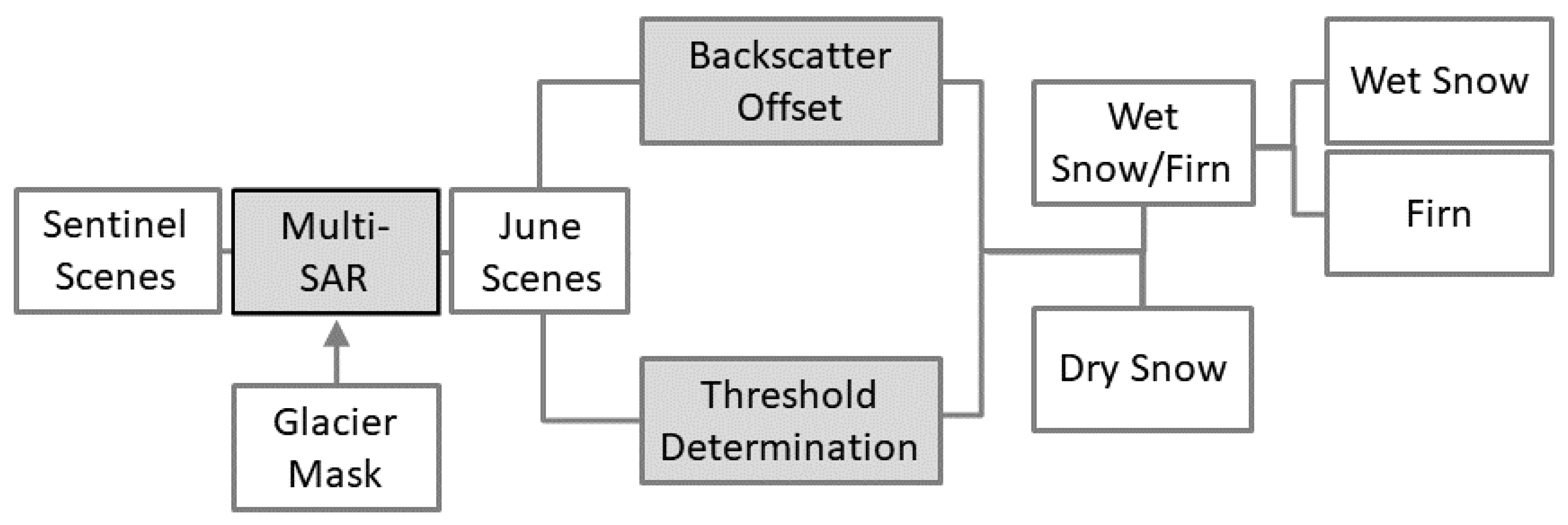
2.2. SAR Data Workflow

For the complex terrain in the investigated area, it is important to discriminate backscatter distributions for assumed homogeneous surface conditions from backscatter dependencies due to various surface conditions such as wet snow cover, firn cover or bare ice. Under the assumption of dry snow being transparent for SAR data in C-band frequency ranges, the only period of homogeneous glacier surface conditions are after melt affected upper elevation ranges and before the lowermost glacier parts become snow free. Otherwise, contributing surfaces have different dielectric permittivities (dry, wet snow, ice) and highly variable surface roughnesses. For the Alpine region discussed here, complete wet snow coverage occurs usually in June each year followed by an upglacier retreat of the SCE during the summer. In the following, we describe data processing for all acquired SAR scenes including statistical analysis of homogeneous backscatter scenes. The workflow to derive transient snowlines from acquired SAR scenes is displayed in Figure 2.

2.2.1. Multi-SAR-System

All acquired SAR data were processed with a pre-processing framework called Multi-SAR-System. The Multi-SAR-System enables processing of SAR data being acquired with different sensors within the same system and output of the processed data in a uniform format. The pre-processing system is implemented at the Earth Observation Center of the German Aerospace Center, Oberpfaffenhofen, Germany. It contains geocoding, radiometric calibration and image enhancement. During geocoding, radar image distortions induced by the side-looking geometry of SAR-systems are corrected using a digital elevation model (DEM). The geometric quality of the geocoding depends on the height accuracy and the resolution of the elevation model. We used an airborne laser scanning DEM with a spatial resolution of 10 m generated between 2006–2010 (data source: Province of Tyrol—data.tirol.gv.at). The next step, after geometric adjustments, was a coarse radiometric calibration. Local topographic variations and sensor position affect not only location, but also the brightness of the radar return [27]. In mountainous terrain, this effect can be reduced with a gamma correction. This approach compares the ratio of individual area parcels of a synthetic image derived from DEM and orbit information with the illuminated SAR images. Due to the integration of backscatter over the area parcels, one S1 scene require about one full day of processing time. For regions with moderate slope angles such as for the glacier areas investigated here, the approximation of the gamma correction based on the local incidence angle using ${\gamma }^0={\beta }^{0}tan\Theta$, ${\gamma }^0$ the backscatter coefficient, ${\beta }^0$ the backscatter in beta naught and $\Theta$ the local incidence angle is sufficient. The processing time using the approximated gamma correction reduces to about 20 min per scene. Our interpolation uses the cubic convolution method on a 17 × 17 pixel raster. The last step of the Multi-SAR-System is the image enhancement to reduce the influence of additive and multiplicative noise contribution. Compared to conventional speckle filtering algorithms, the multi-scale, multi-looking approach applied here adapts the local number of looks to the image content. For heterogeneous surfaces (i.e., mountainous areas), a minimal look number and, consequently, the maximum geometric resolution is necessary to adequately describe surface features. The choice of an appropriate look number is made by the help of a novel perturbation-based noise model that combines both additive and multiplicative noise contributions and automatically adapts to sensor and imaging mode characteristics via the delivered metadata. The result is a very smooth, but detail-preserving multi-looked SAR image representing the local optimal trade-off between geometric resolution and radiometric accuracy. Finally, image values are converted to the standard unit decibel (dB) [28,29].

As a next step, two different masks are applied. The first mask eliminates the radar shadow and layover effects and the second mask removes non-glaciated areas (based on the glacier boundaries of 2009 derived from optical remote sensing data). As a result, we receive SAR data of just the respective glaciated areas described in Figure 1.

2.2.2. Backscatter Variability of Wet Snow Scenes

To determine the variability in ${\gamma }^0$ for homogenous wet snow surfaces, we calculated the coefficient of variation (CV, $CV=\frac{\mu }{\sigma }$, $\mu$ the arithmetic mean and $\sigma$ the standard deviation) per June scene. A low variability in backscatter distribution per glacier areas indicate homogeneous conditions. We set the CV in backscatter to below 20% as criterion for data selection.

Table 3. Determined coefficients of variation for all acquired Sentinel-1 scenes in June between 2015–2018. Respective orbits are described in Table 2.

Platform	Orbit	Date	VH	VV
S1	168	2 June 2015	0.14	0.24
S1	168	8 June 2016	0.10	0.20
S1	168	3 June 2017	0.13	0.25
S1	168	9 June 2017	0.13	0.26
S1	168	15 June 2017	0.14	–
S1	168	21 June 2017	0.15	–
S1	168	4 June 2018	0.13	–
S1	168	10 June 2018	0.14	–
S1	168	16 June 2018	0.15	–
S1	168	28 June 2018	0.15	–
S1	117	10 June 2015	0.13	0.26
S1	117	22 June 2015	0.21	0.44
S1	117	3 June 2015	0.10	0.17
S1	15	15 June 2015	0.11	0.20
S1	15	27 June 2015	0.11	0.18

displays the determined CVs for June scenes in cross- and co-polarization.

Almost all cross-polarized SAR scenes in Table 3 show a CV for June acquisitions of 15% or less. The single exception is the S1 scene being recorded in ascending orbit in 2015. All co-polarized scenes, however, result in a variation significantly higher than for cross-polarized acquisitions and show a much larger range. Such larger ranges indicate less consistency. Consequently, we use only on cross-polarized SAR scenes.

A secondary criterion for data selection is time of acquisition. During the main melt season in August, glacier ice and firn surfaces are very much affected by surficial melt water streams during the day, while early in the morning at 5:30 UTC (local time 7:30) nocturnal refreezing has peaked. Unfortunately, all ascending scenes were acquired at 17:10 UTC (local time 19:10), when it is more likely that strong surface wetting and meltwater runoff can lead to misinterpretation for the extent of wet snow covered areas. Hence, in the following, we will present methodology and results only for descending cross-polarized orbits, which were acquired at 5:30 UTC in the morning (Table 2). We excluded the first S1 June scene in Figure 3b (recorded on 2 June 2015) despite a CV value of 14% (Table 3). The median value of this scene is distinctly higher than for the remaining scenes (Figure 3). We expect that higher elevation ranges for all glaciers were still covered by dry snow and, hence, increase the median backscatter to higher values.

2.2.3. Correction of Systematic Backscatter Offsets

However, cross-polarized wet snow scenes are very homogeneous (Figure 3), and topographic effects very often bias interpretation of satellite data. In addition, very complex topographies, such as mountain glacier regions with various slope aspects, are challenging for space borne acquisitions to interpret. In addition, we relied on a DEM from 2006 for data processing. In particular, at glacier tongues, topography has lowered significantly between time of acquisition and DEM generation. Since we had several acquisitions in June with equal orbits during four years of data acquisition, we could check whether variations to average ${\gamma }^0$ per scene are fully random or very similar for consecutive years and various melt progresses. We calculated for each June SAR scene deviations from the respective median. Deviations in ${\gamma }^0$ being constant in location and independent from melt progress can be attributed as systematic due to topography and incidence angle. Next, we calculated the variance of determined deviations for all June scenes for each pixel. Calculated variances for the nine wet snow scenes below a value of 0.5 indicate that offsets from median are systematic and are corrected for. Figure 4 displays the resulting constant deviations used as backscatter offset correction file. To prevent misinterpretation of snow-free glacier tongues, we set corrections for the GPF and HEF glacier tongues to zero. This file was subtracted from each single S1 scene as additional topography correction. Instead of manually discarding snow-free glacier termini, one can apply automated detection algorithms (e.g., [30]) to minimize influences of already snow free glacier parts. We consider platform effects such as variations in perpendicular baseline or image frame as negligible for the here performed analysis. However, in case such deviations would be significant, the effect per pixel would vary with different baselines and, hence, the pixel variances of different scenes increase.

2.2.4. Threshold Determination

The above selected nine wet snow scenes (Figure 3) are used to calculate wet snow thresholds. We calculated for each scene the upper quartile (75% percentile, upper frame of the boxes (Figure 3) of the backscatter distribution. The arithmetic mean of those upper quartiles is used to discriminate wet snow and wet firn from dry snow and bare ice areas (threshold ${\beta }_1$, black line in (Figure 3). In a second step, we used solely the parts of the wet snow scenes with ${\gamma }^0<{\beta }_1$ and calculated the 95% percentiles per remaining part of the scenes. The arithmetic mean of those percentiles result in threshold ${\beta }_2$ (purple line in (Figure 3). The resulting values are ${\beta }_1=-21.45$ dB (with standard deviation of 0.76 dB) and ${\beta }_2=-22.41$ dB (with standard deviation of 0.18 dB). The determined standard deviations are further used for sensitivity analyses.

For the applied two-step approach, we first analyze for glacier parts being classified as wet using ${\beta }_1$. After correction for systematic backscatter offsets, we subtracted ${\beta }_1$ from each S1 scene resulting in a classification as dry/bare ice (positive values) or wet (negative values). In case the classified wet area is less than 50% of the glacier, we further discriminated for firn and wet snow utilizing ${\beta }_2$. Here, we used again the offset corrected S1 scenes, removed all dry parts classified with ${\beta }_1$ and subtracted the wet areas by ${\beta }_2$. The resulting pixels were classified as wet snow (negative values) and firn (positive values). The proportion of each glacier AOI being either wet or wet snow divided by the whole AOI area results in the WSCAF. Glacier parts, which were covered by dry snow, cannot be distinguished from bare ice areas. As a result, we interpret WSCAF per glacier AOI as accumulation area fraction.

2.3. Processing of Optical and Near-Infrared Remote Sensing Data

Similar to, e.g., Nagler et al. [9] and many other authors, we used L7, L8 and S2 acquisitions to assess the accuracy of the presented SAR workflow on capturing transient snowlines. From now on, we use the term “optical” remote sensing data to abbreviate the usage of Landsat or Sentinel-2 data.

While the SAR data presented here are solely sensitive to wet snow, data within and close to the optical frequency range display brightness differences at the surface. However, cloud coverage often prevents data usage from optical instruments. For instance, in summer 2017, not a single Landsat scene for the here described AOIs could be used for comparison with SAR data. Each Landsat scene for this region was strongly influenced by clouds (a maximum of 20% cloud coverage per glacier was set as cut-off criterion for data usage). For the other observed summer seasons, we were able to make use of eight optical scenes. We used the normalized difference snow index (NDSI) [31,32,33] for automatic classification of snow covered areas for Landsat data and the Level-2A algorithm for Sentinel-2 data [34]. For L8 scenes, we used a threshold of 0.6 and for L7 this threshold had to be increased to 0.88 to obtain reliable results for snow covered areas. Snow classification thresholds for S2 data were increased to 0.16 (2017) and 0.18 (2018) from the given 0.12 [34] to match best the visually inspected snow boundaries. Since coincidences of optical sensor acquisitions and SAR imagery are rare, the quantification of spatial deviations between both data interpretations is difficult. We defined a range of four days prior and four days after each optical acquisition as being reasonable for direct comparison. For the case of new snow events within this time range, data were not used for analysis.

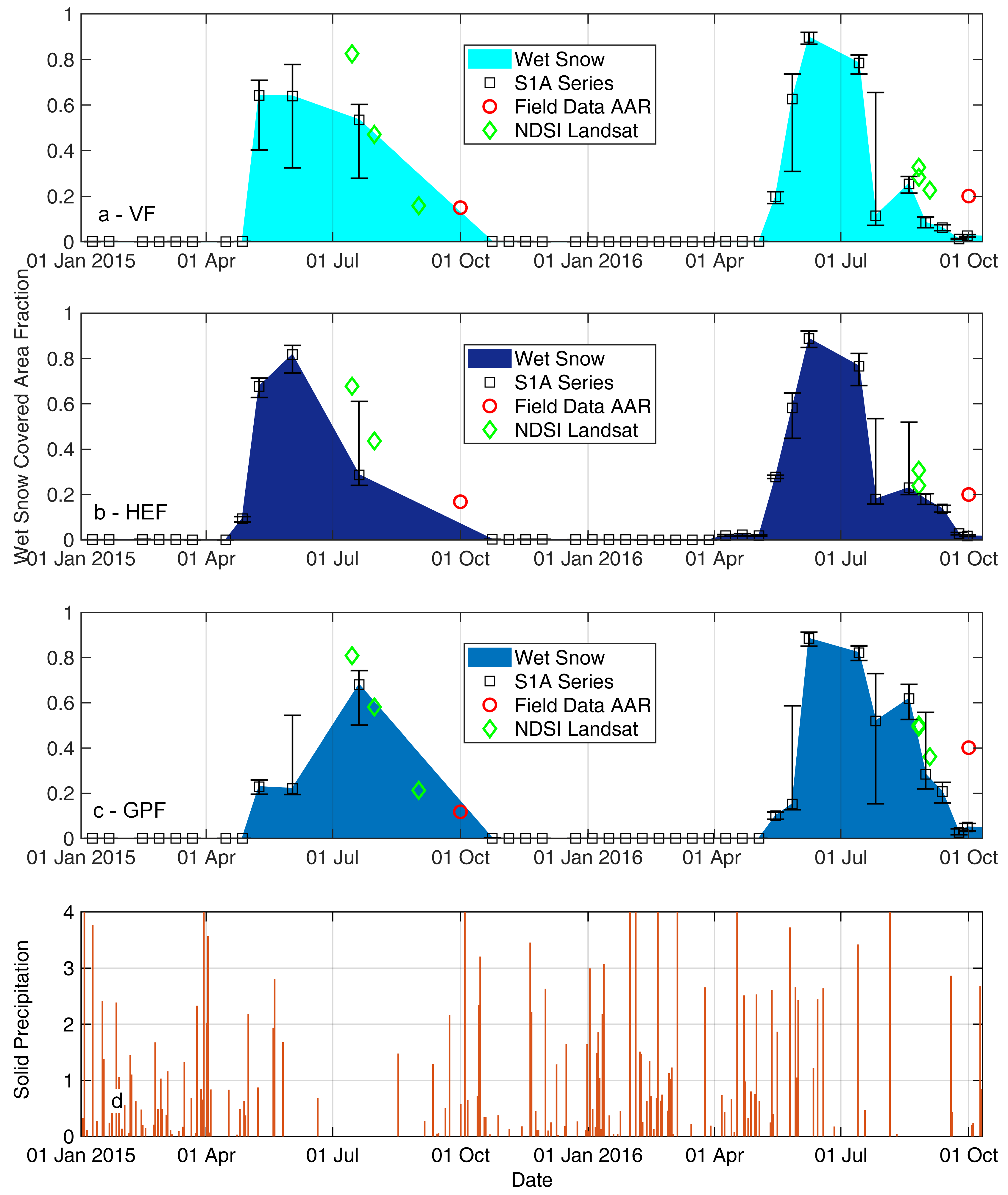
2.4. Annual Minimum Wet Snow Covered Area Extent

For remote sensing data, fixed date acquisitions such as annual mass balance assessments per glaciological year (GY) are difficult to achieve due to overpass rates and priority rankings by the satellite operators. However, more importantly, conditions on the glacier can be very different from year to year at fixed dates. In this study, we propose searching for local minimum in a wet snow extent within a range of five weeks prior to 30 September each year and two weeks after that day. Within this time range, we search for the local minimum in WSCAF for SAR scenes. However, recent new snow falls shortly before a SAR acquisition influence the detected WSCAF drastically. A minimum by early October could arise due to the fact that almost the entire glacier was covered by dry snow and, hence, volume scattering drastically increased. To prevent misinterpretation of derived snowlines, we applied a correction algorithm before minimum search based on observed firn and snowlines from optical data. We used the fact that perennial firn is more resistant to melt than seasonal snow. For the last analyzed S2 scene (16 September 2018), we decreased the snow threshold to 0.0 (instead of 0.18) and determined the area per AOI for reflectivities larger than zero. These areas include, at least, a fraction of the perennial firn coverage per AOI. Since those firn areas were formed in previous years from snow reserves, it is impossible that the SAR detected firn and WSCAF (result of step 1) is below those optical results. We defined that any SAR scene with lower “wet” areas than 75% of this optical reference scene as being influenced by recent new snow. Hence, those scenes were excluded from annual minimum snowline searches. The resulting minimum snowline is used as annual AAR from SAR scenes.

3. Results

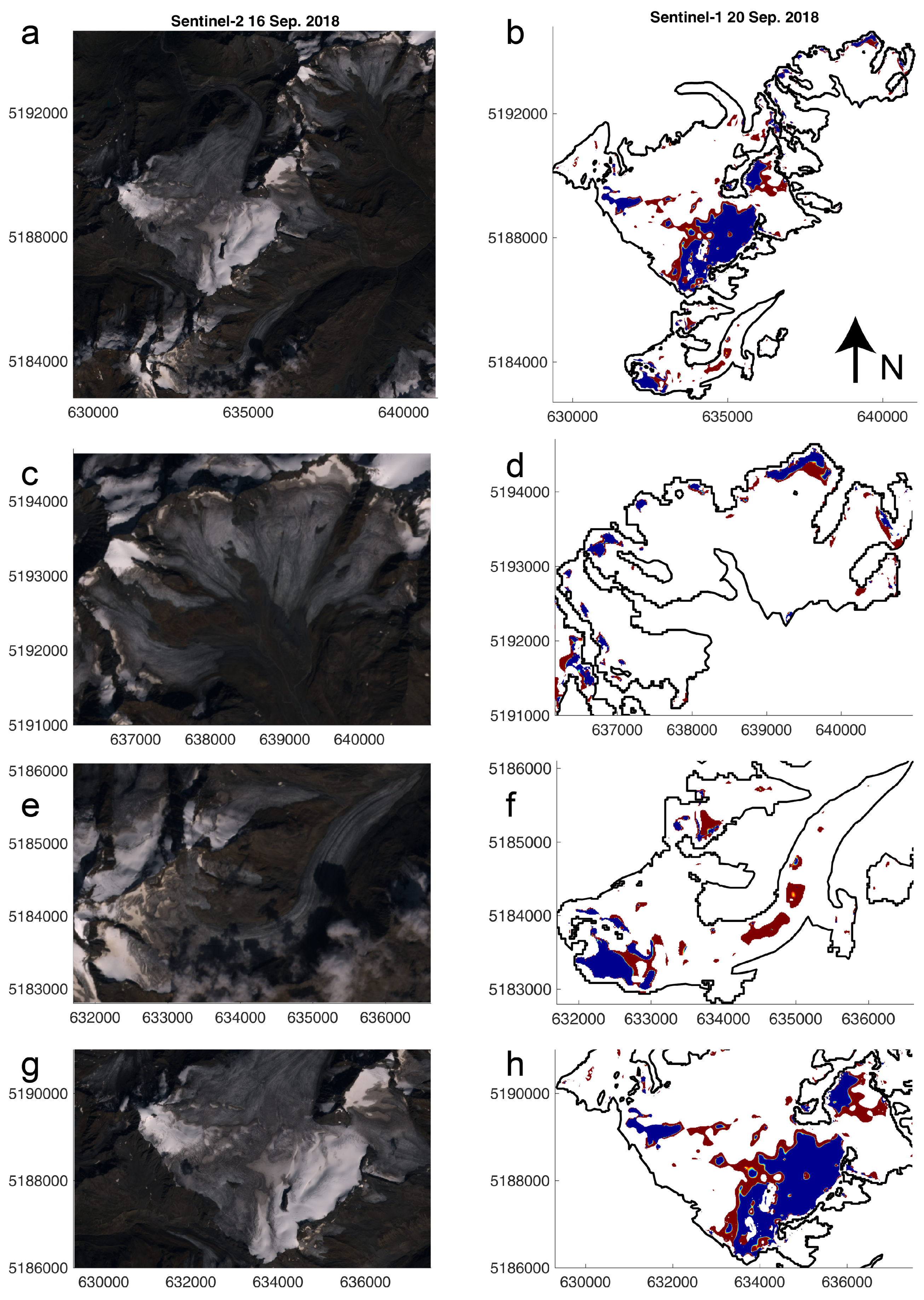
3.1. Wet Snow Covered Area Extent

Figure 5 and Figure 6 display the seasonality of backscatter distributions being above or below the thresholds. For all four observed accumulation seasons (winter periods), snow surface conditions are constantly dry and, hence, WSCAFs are at about zero. Since we determined no changes during periods from January until early April in 2015 and 2016, we minimized data acquisition for this period for the remaining years. From late April to May, the snow surface is starting to becoming wet and reaches towards average WSCAFs in June of 80–90%. June 2015 is an exception, when only 60–70% are reached. However, we could only analyze a single June scene in 2015, which was recorded at the very beginning of the month. After the launch of S1B in spring 2016 and the following commissioning phase, C-band data were available with six days return cycles beginning in late September 2016. The ablation seasons 2017 and 2018 provide a much more detailed view on temporal and spatial changes of WSCAF for all AOIs. WSCAF recession during the ablation season after June is usually very rapid with interruptions by new snow events (Figure 6). New snow events during the ablation season can have a large effect on B [35] due to the short term increase in albedo up to values of 0.9. In summer 2017, two snow fall events can be directly related to sharp increases in WSCAF for all three AOIs. It is possible to detect a peak in WSCAFs for 15 July 2017 for all three AOIs, while respective amplitudes are different. VF decreases after 1 July 2017 from about 80% WSCAF to below 20%, the same occurs for HEF, whereas GPF remains at 60%. The corresponding snow fall events were recorded for 6 and 7 July. However, no increase in WSCAF as a consequence of this recent new snow is recognizable for the subsequent SAR analysis on 9 July 2017. Temperatures remained low and, hence, this recent snow was not affected by melt. Shortly before the following SAR image, snow melt changed ${\gamma }^0$ resulting in a local peak of derived WSCAF. The next peak in WSCAF observed at 20 August 2017 is related to new snow as well. Again, amplitudes are significantly larger for GPF in comparison with VF and HEF. In summer 2018, WSCAFs decrease to very low values for VF and HEF with only slight interruptions. Solely, the new snow event in late August this summer has a remarkable effect on WSCAFs for those two AOIs. GPF, however, is characterized by two additional peaks in July and mid August. At the Ultrasonic location on VF, no snow fall could be recognized. At least for mid August, we noticed a liquid precipitation event at lower elevations, while higher glacier regions received new snow. The mostly northerly exposed GPF, which has a large flat plateau above 3100 m a.s.l., results in a WSCAF increase to above 30% for this SAR scene.

The applied two-step approach has an effect on sensitivity displayed through errorbars. Large errorbars can—in most cases—be attributed to recent new snow precipitations (Figure 5 and Figure 6). After a snow fall event, the area extent of wet snow change across the criterion of 50% for the application of the ${\beta }_2$, which, as a consequence, can have a strong effect on determined WSCAFs. This is regularly the case for GPF.

For comparison with optical remote sensing data, four SAR scenes were available, which fulfill the requirements of a temporal offset of maximum $\pm 4$ days. The root mean square (RMS) deviation for the four periods for VF and GPF and only two periods for HEF (due to cloud coverage) results in 8.5% difference. This deviation is insensitive to subtraction of standard deviations from ${\beta }_1$ and ${\beta }_2$ (RMS deviation of 7.8%) but increases to a RMS deviations of 18.1% when applying the higher threshold range. Unfortunately, a new snow event during the night of 14 to 15 August 2018 above roughly 3200 m a.s.l. had a significant influence on the SAR detected WSCAF at 15 August in the morning. This new snow was already melted before the acquisition of optical imagery the subsequent morning. Discarding this SAR value from RMS analysis leads to deviations of only 4.9% with an sensitivity range of 4.7–13.5%

We used changes in snow/ice height measured at the lower glacier tongue of VF as a proxy to assess ice melt progress until the end of the respective GY. For all three analysed ablation seasons, the depicted annual minimum in snowline from SAR data was before the respective end of the GY. To relate ablation progress, we compare ice heights for these dates with 30 September each year. In 2016, the ice surface lowered by −27 cm from 12 September until 30 September (to −2.66 m). The subsequent year, the offset in ice surface reduced to 19 cm for an even longer time span (26 August–30 September) with an annual ablation of −3.1 m at the end of the GY. Finally, in 2018, we observed a surface lowering of 28 cm for only ten days between SAR minimum and end of GY (−4.53 m). All surface height values are related to the start of the respective GY, which is set to a surface height of 0.0 m. No annual mass balance assessment for GPF are conducted so far.

Offsets to estimates from field investigations are presented in

Table 4. Annual accumulation area ratio (AAR) estimates from field data and annual minimum in wet snow covered area fraction determined from Sentinel-1 (S1) scenes with date of acquisition in brackets per glaciological year (GY) and area of interest Vernagtferner (VF) and Hintereisferner (HF). All values are presented in percent (%).

	VF			HEF
GY	Field Data	S1	Field Data	S1
2015/16	20.0	6.2 (12 Sep.)	20.0	13.7
2016/17	12.0	3.9 (26 Aug.)	3.2	9.7
2017/18	–	3.9 (20 Sep.)	7.1	6.2

. RMS deviation result in 8.2% for HEF and VF for a sample size of five.

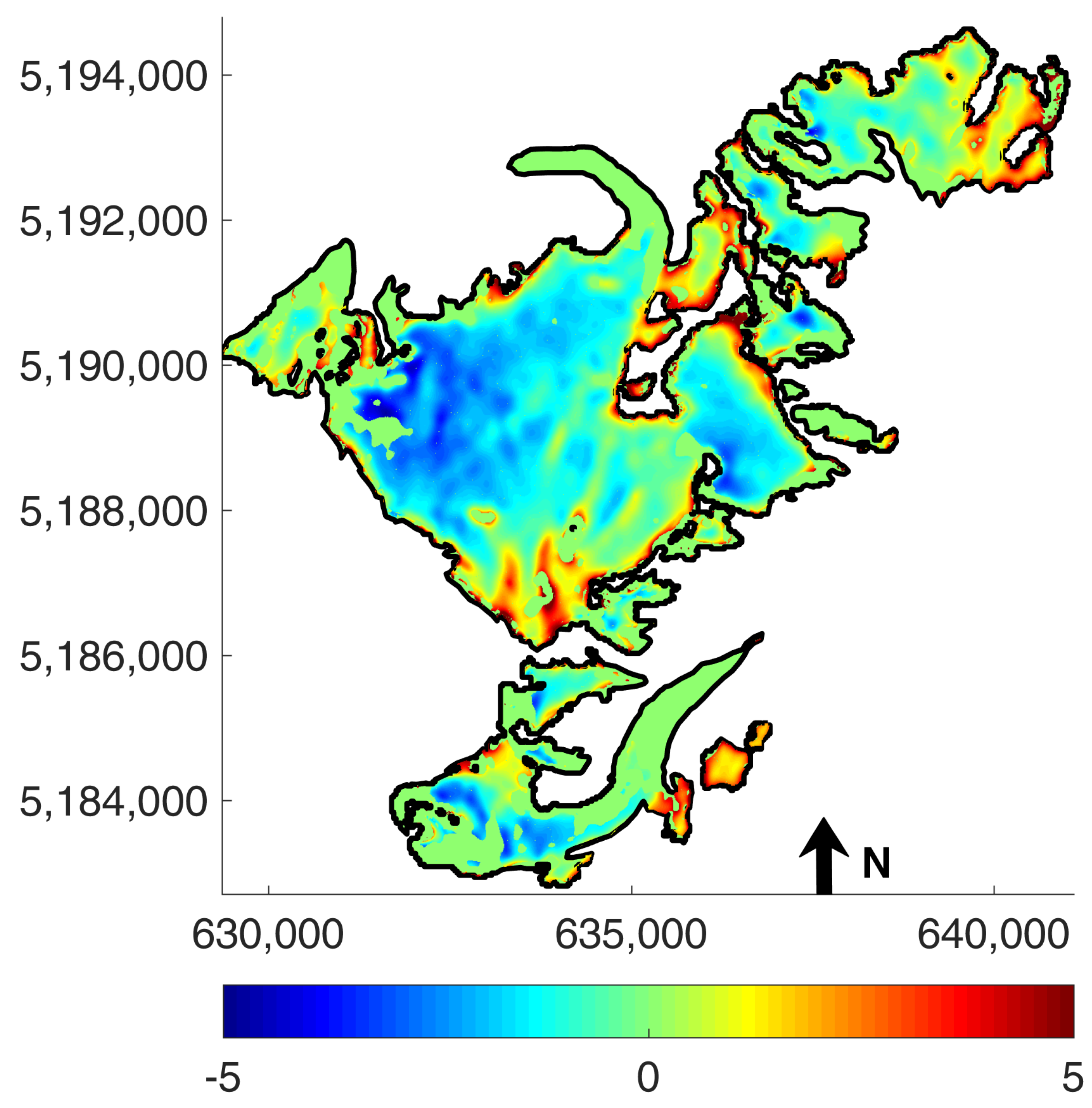
3.2. Discriminating Firn and Wet Snow

Only reliable discriminations between wet snow and firn enable derivation of annual AAR for various glaciers. We analyze for accuracies in wet snow–firn discrimination by a short in situ GPS transect for the transient snowline on VF. For this 303 m long transect discriminating firn from wet snow, we determined an average offset for the SAR-derived transient snowline of 35 m and for optical data this offset decreases to 19 m. In addition, 35 m correspond to about 3–4 pixels for a 10 m × 10 m SAR resolution. The respective S2 data providing optical data has the same ground resolution. However, optical data have been recorded four days prior to ground truth and S1 data. Apart from the short 300 m in situ line, qualitatively, we demonstrate agreement of optical data with SAR data in Figure 7. It is inevitable that disagreement between optical data and SAR data occur, but, in general, this overview confirms the 3–4 pixel accuracy determined for the in situ data.

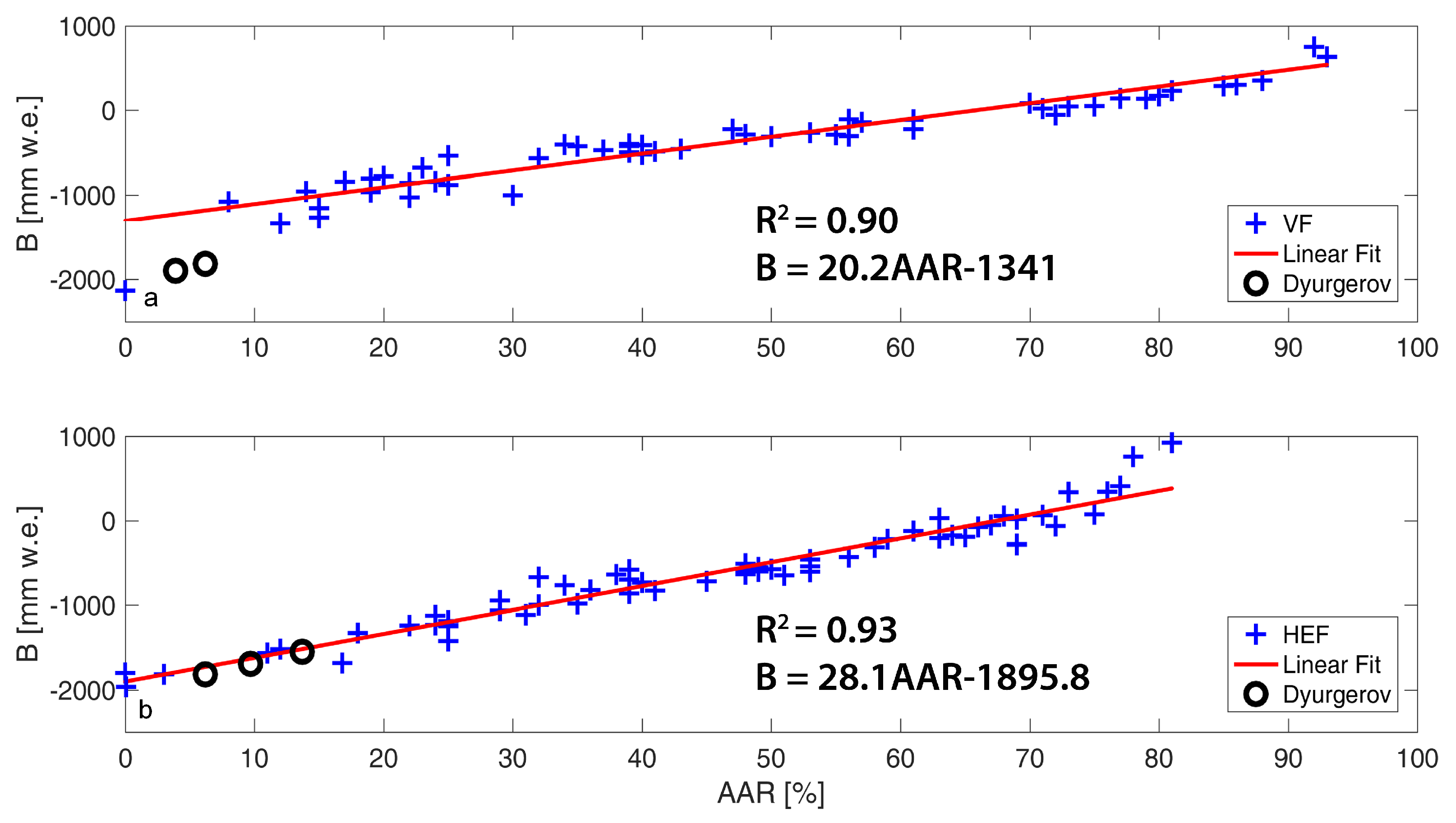
3.3. From Minimum Wet Snow Extent to Mass Balances

For Vernagtferner and Hintereisferner, long-term summer and winter mass balance series exist (VF: 1964/65–2016/17; HEF: 1952/53–2017/18; [21,22]) (e.g., [36]). We plotted relationships of AAR and mass balance (B) for VF and HEF in Figure 8. It is clearly visible that a linear fit matches the relation between B and AAR adequately. Coefficients of determination (R${}^2$) are high reaching $R^2=0.93$ for HEF with a sample size of 66 years and a range of 0% to above 80% in AAR. The $R^2=0.90$ for VF is slightly lower with a lower sample size of 53 years and a higher range from 0% to more than 90% in AAR. Calculated RMS deviations to the linear approximation for both glaciers are at 212 mm w.e. for VF and 154 mm w.e. for HEF.

Such long-term mass balance series with reliable relationships of AAR and B enable direct conversion from SAR determined annual AAR to B (Figure 8,

Table 5. Annual mass balance (B) estimates from field data and annual minimum accumulation area ratios (AAR) determined from Sentinel-1 (S1) scenes. For conversion from accumulation area ratio (AAR) to B, we used the formulations of the linear fit for Vernagtferner (VF) and Hintereisferner (HEF) displayed in Figure 8, Dyurgerov’s average relationship [37] (Dyu) for all glaciers and specified just for the Eastern Alps (Dyu EAlps). All mass balance values are presented in millimeter water equivalent (mm w.e.).

	VF				HEF
GY	Field Data	Linear Fit	Dyu	Dyu EAlps	Field Data	Linear Fit	Dyu	Dyu EAlps
2015/16	−781	−1216	−1814	−1406	−1263	−1511	−1547	−1223
2016/17	−1335	−1262	−1896	−1463	−1826	−1623	−1689	−1321
2017/18	–	−1262	−1896	−1463	−1963	−1722	−1814	−1406

). Deviations to observed B values from field data are highly variable from +435 mm w.e. to −73 mm w.e. for VF and from +248 mm w.e. to −241 mm w.e. for HEF using S1 data. In absolute deviations, those numbers average to 254 mm w.e. for VF and 231 mm w.e. for HEF. Such average offsets are above the given accuracy ranges of the linear approximation (in RMS deviation); however, sample numbers are very low.

Instead of an individually derived linear relationship for each single glacier, Dyurgerov et al. [37] used 99 index glaciers and came up with an average relationship for AAR and B. We included results from this average formula in Table 5 and Figure 8, together with a relationship derived from just Eastern Alpine glaciers (11 glaciers with B and AAR values) listed in [37]. For both glacier areas and most observation years, offsets in mass balance values surpass the given uncertainty range for direct measurements with the glaciological method significantly. Dyurgerov’s approximation result in an average absolute offset for VF of 797 mm w.e.. However, the rather typically shaped valley glacier area of HEF matches the general approach by Dyurgerov significantly better. Average absolute offsets sum up to 190 mm w.e.. An approximation established just for Eastern Alpine glaciers does not decrease offsets. Calculated average absolute deviations are 377 mm w.e. for VF and 367 mm w.e. for HEF. The sample number for the Eastern Alps is very low with just 11 glaciers; however, the $R^2$ of the linear approximation reaches 0.79 and the RMS deviation for the 11 glaciers results in 179 mm w.e.

4. Discussion

4.1. Uncertainty Analysis and Limitations

All presented data on AAR and mass balances include uncertainties. It is difficult to quantitatively assess the respective error per observation technique. The assessment of annual AAR is usually more subject to uncertainties. For a glacier-wide estimate of AAR, peaks above the glacier or airplane observations are beneficial to prevent misclassification of recent and perennial firn. For very small accumulation areas left after a strong ablation summer, correct assessments depend on accumulation stakes and direct observations. This is especially the case for a strong negative year in terms of mass balance subsequent to a rather less negative year. Extrapolation for the whole glacier area and interpolation in between observations is challenging.

The introduced two-step thresholding based on wet snow scenes (Section 2.2.4) does include some local uncertainties. We observed areas that showed ${\gamma }^0$ values below the respective threshold, which certainly were snow free in late August and September (Figure 7f). Such areas usually were present on HEF and GPF and, for both glaciers, limited to the glacier tongue regions. It appears from comparing images with and without applied correction for systematic backscatter offsets (Section 2.2.3) that these areas deviate strongly from median ${\gamma }^0$ (Figure 4). The applied backscatter enhancement was probably not sufficient to correct for these deviations. In general, rough surfaces like bare glacier ice increase the reflected backscatter [38] for SAR data due to enhanced diffusive scattering. We can only speculate about the reasons of this amplification of the decline in ${\gamma }^0$. Although the applied DEM does not indicate layover and shadowing for those areas, we assume that the steep topography has some effects, especially because the DEM used for SAR processing was generated up to more than ten years prior to acquisition dates and the glacier surface lowered significantly within this time period.

In general, the presented RMS deviations of WSCAF to results from optical remote sensing imagery are below 10%. However, sample sizes for comparison are low. We only found four optical scenes, which were recorded shortly prior or after an S1 data acquisition. For the three analyzed AOIs, the calculated RMS values represent not very resilient statistical values. An accuracy of below 10% is encouraging, however, considering the fact that conventional methods rely on data inter- and extrapolation or are hampered by cloud coverage. Since for three consecutive years only very few optical scenes were available during the ablation periods, SAR data offer a significant progress in determination of annual and seasonal transient snowlines and, consequently, AAR. Six days of overpass rates enabled already almost complete coverage for the ablation seasons 2017 and 2018 with a high temporal resolution.

In addition, such a high temporal resolution demonstrates difficulties in data interpretation by simple thresholding. The sensitivity of WSCAF results on deviations in thresholds is in most cases very low. Derived uncertainty ranges are at $\pm 2\%$, which corresponds to the sizes of data markers in Figure 5 and Figure 6. However, some errorbars cross the set 50% WSCAF criterion for different thresholding and, consequently, sensitivity analysis are performed over more than 1 dB. Especially for GPF with its flat plateau above 3100 m a.s.l., fluctuation in thresholding occurs more frequently. In most cases, sensitivity increases shortly after a recent new snow event. New snow has two different effects on WSCAF classification from SAR data. If the recent new snow coverage experiences melt, the WSCAF will significantly increase. In addition, dry new snow increases volume scattering from the surface, and, consequently, resulting backscatter values of former wet surfaces may reach above the set threshold values. Hence, determined WSCAF decreases. Such occurrences can be observed for instance at the end of each GY or shortly after 01 October. Here, WSCAFs reduce to roughly 0%. Disregarding this effect would result in misclassification of minimal wet snow extents per ablation season. The applied criterion for the search of minimal extents in wet snow each year seems to work properly to neglect such dry snow covered minimum in WSCAF.

Since large large threshold sensitivities—displayed via errorbars—can be related to new snow events or WSCAFs at about 50%, such values are prone to errors and uncertainties. For comparison with optical remote sensing data or for determination of annual AAR values, we recommend focusing on SAR data being insensitive to threshold variations. For S1 data with six days return cycles, this would reduce seasonal coverage by one (2017) to four (2018) scenes for VF and limit the temporal coverage for GPF to only half of the previously analyzed scenes.

4.2. Discrimination of Wet Snow and Firn

Not only do dielectric permittivities change backscatter emissivity of surfaces, but surface roughness as well (e.g., [38]). Wet snow and wet firn have similar dielectric permittivities, if the volumetric liquid water content (${\theta }_w$) is equal and impurities are negligible (s = snow, f = firn, ${\rho }_s=360$ kg/m${}^3$, ${\theta }_w=0.04$, ${\rho }_f=500$ kg/m${}^3$; ${ϵ}_s=2.8$, ${ϵ}_f=3.2$). Concave furrows as a result of melt and sublimation processes on the snow surface increase with continuing ablation, especially, for the inner Alpine dry regions with intensified sublimation observed here. According to the Rayleigh criterion, surfaces are considered as rough for SAR data, if $h>\lambda /8cos\delta$ [39] with h the height of the surface features, $\delta$ the given incidence angles and $\lambda$ the wavelength of the respective platform. This leads to a roughness sensitivity of roughly $h>8$ mm for C-band data. For soil surfaces, [40,41] found that SAR backscatter increases are most sensitive to changes in surface roughness of $0<Zs\le 0.4$ with $Zs=s^2/l$, the roughness parameter where s is the root mean square of surface height h and l the correlation length. For reasonable s and l values, we derive $Zs$ as displayed in Figure 9. It is obvious that backscatter increases are caused by increases in s between 0 cm to about 7 cm for correlation lengths observed in the field. An increase in surface roughness up to 7 cm can usually be observed for transitions from seasonal snow to firn (see Figure A1). For the short in situ transect separating firn and wet snow recorded the same day as a SAR acquisition, we found sufficient agreement of 3–4 pixels. However, the difference of the thresholds separating firn and snow is close to the given resolution limits of S1 data.

4.3. SAR Data for Application in Seasonal Mass Balance Estimates

It remains debatable to which degree field assessments of AAR are accurate. Usually, no continuous snowline data are available for field assessments. Accumulation area ratios for alpine glaciers are commonly estimated according to elevation ranges and stake readings. However, without a long-term time series of direct measurements, no reliable AAR to B relationship can be established.

The long time series of mass balance observations for HEF and VF with data distributions from 0% to almost 100% in AAR enable for deriving a resilient formulation for the AAR to B correlation. Inserting SAR based annual AAR in a linear fit results in average offsets of 200–300 mm w.e. This is above given uncertainty ranges for systematic errors of direct mass balance measurements and above the uncertainty of the linear approximation for each glacier. Two limiting factors reduce accuracy of such an approach: (i) for both time series, the linear relationship resulted in average errors larger than 100 mm w.e. (RMS deviation VF 212 mm w.e., HEF 154 mm w.e.); and (ii) the date of SAR acquisition is crucial. The approach by Dyurgerov et al. [37] with a generalized relationship over 99 glaciers is not sufficient for the rather flat and southerly exposed VF to accurately determine B just from AAR observations. For HEF, as a more typical valley glacier, this generalized approximation provides better estimates on B for the three observed GYs. Reducing the globally derived glacier relationship of B and AAR to the geographical region of the Eastern Alps provides larger deviations for HEF and decreases the offset for VF. However, data used in [37] have a temporal extent until early 2000. Including the strong ablation seasons within the last decade most likely will influence the derived relationship of AAR and B.

Observation of the temporal evolution of the transient snowline with SAR data is reliably possible with the presented algorithm for the glaciers of the Rofental, Austria. Single scenes are very difficult to interpret, since the respective acquisition can be biased by recent new snow precipitation. However, data interpretation benefit from time series of SAR observations with high temporal resolution and thus misinterpretation due to new snow events is limited. In addition, the applied criteria for the search of annual minimum reliably exclude scenes covered by recent dry snow.

Whether the proposed two-step approach for discriminating wet snow and firn is applicable for other areas in various latitudes or climatological regions remains unknown. For glaciers outside middle latitudes without pronounced seasonality (e.g., high latitudes and very high altitudes), remote sensing data only provide snapshots depending on the time of acquisition and prevailing weather conditions. The derived data on WSCAF for such geographical regions has no or limited significance on ablation progress. As a first step for each region, ${\gamma }^0$ values for wet snow conditions have to be analyzed for all acquired orbits and polarization channels. In case sufficient amounts of SAR scenes fully covered by wet snow are available, the processing routines as described here can be implemented into automatic data analysis resulting in an output of just WSCAF per acquisition.

However, such data analysis does not directly lead to surface mass balance per glacier area. The relationship of annual AAR to B is usually significantly different for each glacier and relies on individual topography, elevation range and aspect. Empirical approaches such as the one proposed by Drolon et al. [42] are less influenced by individual glacier topographies and do not need long-term data series. However, [42] focuses rather on large scale accuracies than on individual glaciers and use optical satellite data with the named restrictions on visibility. In addition, presented uncertainties on annual mass balance values are rather large.

Other SAR platforms using X- or L-band sensors are most likely applicable for such an analysis as well (see [43]). Again, for proposed workflow described here, it is prerequisite that wet snow scenes can be used to derive threshold values and to apply topographic corrections. The main disadvantage for those platforms is the temporal resolution with return cycles of more than 10 days. For instance, over several years of ALOS-PALSAR-1 and 2 data, we could only acquire three June scenes for the region analyzed here.

5. Conclusions

This case study presents a two-step workflow using thresholds to discriminate wet snow and firn for SAR data. In a first step, the workflow distinguishes dry and wet surfaces and subsequently analyzes wet surfaces for wet snow and firn with a second threshold value. Deviations to the extent of snow covered areas derived from visual and shortwave infrared channels are less than 10% (8.5%) in area for C-band data. WSCAF is sensitive to increases in threshold values, which can lead to offsets up to 18.1%. Average offsets of annual minimum in WSCAF from SAR data and field data on annual AAR are at below 10% (8.2%) as well for three observed GYs and three different glacier areas. For analysis, we included 12 individual glaciers covering a wide range of elevation and exposition as well as area extent. All glaciers are located within the Rofental, Austria. For two glaciers within this study, long-term mass balance series are available. We used these time series to establish linear relationships between AAR and B and compared field measurements on B with outcomes for the relationships for SAR derived AAR values. Deviations between field assessments of B and SAR derived values are at 200–300 mm w.e. on average. Such results are not an improvement compared with conventional measurements but enable mass balance estimates for regions not accessible or too dangerous for conventional mass balance observations. Results are very encouraging and demonstrate the feasibility of the proposed workflow to derive AAR from SAR data. In addition, we could show that glacier surface conditions during the melt season can be quasi-continuously be monitored using S1 SAR data, which is essential for glacier runoff modeling. Implementation of this workflow for other regions worldwide has to be analyzed with extended SAR data acquisitions. However, apart from SAR data, solely the availability of DEMs with sufficient accuracy is required to apply the proposed workflow.

References

1. Zemp, M.; Thibert, E.; Huss, M.; Stumm, D.; Rolstad Denby, C.; Nuth, C.; Nussbaumer, S.U.; Moholdt, G.; Mercer, A.; Mayer, C.; et al. Reanalysing glacier mass balance measurement series. Cryosphere 2013, 7, 1227–1245. [Google Scholar] [CrossRef] [Green Version]
2. WGMS. Global Glacier Change Bulletin No. 1 (2012–2013); ICSU(WDS)/IUGG(IACS)/UNEP/UNESCO/WMO; World Glacier Monitoring Service: Zurich, Switzerland, 2015. [Google Scholar]
3. Benn, D.I.; Evans, D.J.A. Glaciers & Glaciation; Arnold: London, UK, 2006. [Google Scholar]
4. Nagler, T.; Rott, H. Retrieval of wet snow by means of multitemporal SAR data. IEEE Trans. Geosci. Remote Sens. 2000, 38, 754–765. [Google Scholar] [CrossRef]
5. Parajka, J.; Blöschl, G. The value of MODIS snow cover data in validating and calibrating conceptual hydrologic models. J. Hydrol. 2008, 358, 240–258. [Google Scholar] [CrossRef]
6. de Ruyter Wildt, M.S.; Oerlemans, J.; Björnsson, H. A method for monitoring glacier mass balance using satellite albedo measurements: Application to Vatnajökull, Iceland. J. Glaciol. 2002, 48, 267–278. [Google Scholar] [CrossRef]
7. Cogley, J.G.; Hock, R.; Rasmussen, L.A.; Arendt, A.A.; Bauder, A.; Braithwaite, R.J.; Jansson, P.; Kaser, G.; Möller, M.; Nicholson, L.; et al. Glossary of Glacier Mass Balance and Related Terms. IHP-VII Technical Documents in Hydrology No. 86; IACS Contribution No. 2; UNESCO-IHP: Paris, France, 2011; p. 114. [Google Scholar]
8. Adam, S.; Pietroniro, A.; Brugman, M. Glacier snow line mapping using ERS-1 SAR imagery. Remote Sens. Environ. 1997, 61, 46–54. [Google Scholar] [CrossRef]
9. Nagler, T.; Rott, H.; Ripper, E.; Bippus, G.; Hetzenecker, M. Advancements for Snowmelt Monitoring by Means of Sentinel-1 SAR. Remote Sens. 2016, 8, 348. [Google Scholar] [CrossRef]
10. Heilig, A.; Mitterer, C.; Schmid, L.; Wever, N.; Schweizer, J.; Marshall, H.P.; Eisen, O. Seasonal and diurnal cycles of liquid water in snow-Measurements and modeling. J. Geophys. Res. Earth Surf. 2015, 120, 2139–2154. [Google Scholar] [CrossRef] [Green Version]
11. Baghdadi, N.; Gauthier, Y.; Bernier, M. Capability of Multitemporal ERS-1 SAR Data for Wet-Snow Mapping. Remote Sens. Environ. 1997, 60, 174–186. [Google Scholar] [CrossRef]
12. König, M.; Winther, J.G.; Isaksson, E. Measuring snow and glacier ice properties from satellite. Rev. Geophys. 2001, 39, 1–27. [Google Scholar] [CrossRef] [Green Version]
13. Jaenicke, J.; Mayer, C.; Scharrer, K.; Münzer, U.; Gudmundsson, Á. The use of remote-sensing data for mass-balance studies at Mýrdalsjökull ice cap, Iceland. J. Glaciol. 2006, 52, 565–573. [Google Scholar] [CrossRef] [Green Version]
14. Huang, L.; Li, Z.; Tian, B.s.; Chen, Q.; Liu, J.L.; Zhang, R. Classification and snow line detection for glacial areas using the polarimetric SAR image. Remote Sens. Environ. 2011, 115, 1721–1732. [Google Scholar] [CrossRef]
15. Brown, I.A. Synthetic Aperture Radar Measurements of a Retreating Firn Line on a Temperate Icecap. IEEE J. Sel. Top. Appl. Earth Observ. Remote Sens. 2012, 5, 153–160. [Google Scholar] [CrossRef]
16. Barry, R.G.; Gan, T.Y. The Global Cryosphere: Past, Present, and Future; Cambridge University Press: Cambridge, UK, 2011. [Google Scholar]
17. Huss, M.; Sold, L.; Hoelzle, M.; Stokvis, M.; Salzmann, N.; Farinotti, D.; Zemp, M. Towards remote monitoring of sub-seasonal glacier mass balance. Ann. Glaciol. 2013, 54, 75–83. [Google Scholar] [CrossRef] [Green Version]
18. Lambrecht, A.; Kuhn, M. Glacier changes in the Austrian Alps during the last three decades, derived from the new Austrian glacier inventory. Ann. Glaciol. 2007, 46, 177–184. [Google Scholar] [CrossRef]
19. Sentinel-1Team. Sentinel-1 User Handbook; European Space Agency: Frascati, Italy, 2013. [Google Scholar]
20. Braun, L.; Reinwarth, O.; Weber, M. Der Vernagtferner als Objekt der Gletscherforschung. Zeitschrift f. Gletscherkunde und Glazialgeologie 2011, 45/46, 85–104. [Google Scholar]
21. Geodesy; Glaciology. Kenngrößen des Massenhaushaltes des Vernagtferners für den Zeitraum 1964 bis 2015. Available online: http://glaziologie.de/massbal/index.html (accessed on 9 January 2017).
22. WGMS. WGMS Fluctuations of Glaciers Browser. Available online: http://wgms.ch/fogbrowser/ (accessed on 9 January 2017).
23. Oestrem, G.; Stanley, A. Glacier Mass Balance Measurements: A Manual for Field and Office Work; NHRI Science Report 4; National Hydrology Research Institute: Ottawa, ON, Canada, 1969. [Google Scholar]
24. Zemp, M.; Hoelzle, M.; Haeberli, W. Six decades of glacier mass-balance observations: A review of the worldwide monitoring network. Ann. Glaciol. 2009, 50, 101–111. [Google Scholar] [CrossRef]
25. Jansson, P. Effect of Uncertainties in Measured Variables on the Calculated Mass Balance of storglaciaren. Geogr. Ann. Ser. A Phys. Geogr. 1999, 81, 633–642. [Google Scholar] [CrossRef]
26. Funk, M.; Morelli, R.; Stahel, W. Mass balance of Griesgletscher 1961–1994: Different methods of determination. Zeitschrift f. Gletscherkunde und Glazialgeologie 1997, 33, 41–55. [Google Scholar]
27. Small, D. Flattening Gamma: Radiometric Terrain Correction for SAR Imagery. IEEE Trans. Geosci. Remote Sens. 2011, 49, 3081–3093. [Google Scholar] [CrossRef]
28. Schmitt, A.; Wendleder, A.; Hinz, S. The Kennaugh element framework for multi-scale, multi-polarized, multi-temporal and multi-frequency SAR image preparation. ISPRS J. Photogramm. Remote Sens. 2015, 102, 122–139. [Google Scholar] [CrossRef] [Green Version]
29. Bertram, A.; Wendleder, A.; Schmitt, A.; Huber, M. Long-term Monitoring of water dynamics in the Sahel region using the Multi-SAR-System. Int. Arch. Photogramm. Remote Sens. Spat. Inf. Sci. 2016, XLI, 313–320. [Google Scholar] [CrossRef]
30. Otsu, N. A Threshold Selection Method from Gray-Level Histograms. IEEE Trans. Syst. Man Cybern. 1979, 9, 62–66. [Google Scholar] [CrossRef]
31. Dozier, J. Spectral signature of alpine snow cover from the landsat thematic mapper. Remote Sens. Environ. 1989, 28, 9–22. [Google Scholar] [CrossRef]
32. Hall, D.K.; Riggs, G.A.; Salomonson, V.V. Development of methods for mapping global snow cover using moderate resolution imaging spectroradiometer data. Remote Sens. Environ. 1995, 54, 127–140. [Google Scholar] [CrossRef]
33. Singh, V.P.; Singh, P.; Haritashya, U.K. (Eds.) Encyclopedia of Snow, Ice and Glaciers; Encyclopedia of Earth Sciences Series; Springer: Dordrecht, The Netherlands, 2011. [Google Scholar]
34. ESA—Sentinel Online. Level-2A Algorithm Overview. 2018. Available online: https://earth.esa.int/web/sentinel/technical-guides/sentinel-2-msi/level-2a/algorithm (accessed on 6 December 2018).
35. Oerlemans, J.; Klok, E.J. Effect of summer snowfall on glacier mass balance. Ann. Glaciol. 2004, 38, 97–100. [Google Scholar] [CrossRef]
36. Charalampidis, C.; Fischer, A.; Kuhn, M.; Lambrecht, A.; Mayer, C.; Thomaidis, K.; Weber, M. Mass-Budget Anomalies and Geometry Signals of Three Austrian Glaciers. Front. Earth Sci. 2018, 6, 205. [Google Scholar] [CrossRef]
37. Dyurgerov, M.; Meier, M.F.; Bahr, D.B. A new index of glacier area change: A tool for glacier monitoring. J. Glaciol. 2009, 55, 710–716. [Google Scholar] [CrossRef]
38. Mattia, F.; Le Toan, T.; Souyris, J.C.; de Carolis, C.; Floury, N.; Posa, F.; Pasquariello, N.G. The effect of surface roughness on multifrequency polarimetric SAR data. IEEE Trans. Geosci. Remote Sens. 1997, 35, 954–966. [Google Scholar] [CrossRef]
39. Deroin, J.P.; Company, A.; Simonin, A. An empirical model for interpreting the relationship between backscattering and arid land surface roughness as seen with the SAR. IEEE Trans. Geosci. Remote Sens. 1997, 35, 86–92. [Google Scholar] [CrossRef]
40. Zribi, M.; Dechambre, M. A new empirical model to retrieve soil moisture and roughness from C-band radar data. Remote Sens. Environ. 2003, 84, 42–52. [Google Scholar] [CrossRef]
41. Zribi, M.; Gorrab, A.; Baghdadi, N. A new soil roughness parameter for the modelling of radar backscattering over bare soil. Remote Sens. Environ. 2014, 152, 62–73. [Google Scholar] [CrossRef] [Green Version]
42. Drolon, V.; Maisongrande, P.; Berthier, E.; Swinnen, E.; Huss, M. Monitoring of seasonal glacier mass balance over the European Alps using low-resolution optical satellite images. J. Glaciol. 2016, 62, 912–927. [Google Scholar] [CrossRef]
43. Floricioiu, D.; Rott, H. Seasonal and short-term variability of multifrequency, polarimetric radar backscatter of Alpine terrain from SIR-C/X-SAR and AIRSAR data. IEEE Trans. Geosci. Remote Sens. 2001, 39, 2634–2648. [Google Scholar] [CrossRef]
Sample Availability: S1 and S2 data can be downloaded from the respective webpages of Copernicus Services, Landsat data can be obtained through GLOVIS USGS. Processed S1 results are available from the authors on request.
Figure 1. Study area Hinteres Ötztal with named glaciers. Area margins are color coded for the three areas of interest Vernagtferner (VF), Hintereisferner (HEF) and Gepatschferner (GPF). The background image is a Landsat-8 band 8 composite from September 2016. The red rectangle within the inset displays the location of the study area. Coordinates are given in UTM with datum WGS 1984.
Geosciences 09 00069 g001
Figure 2. Workflow for the classification of wet and dry snow and firn based on Sentinel-1 data. Grey shaded boxes indicate data processing.
Geosciences 09 00069 g002
Figure 3. Box plots of backscatter distributions of all recorded cross-polarized June acquisitions in descending orbits with calculated coefficients of variation below 20% in Table 3. The red horizontal lines within the boxes represent the median in γ 0 , the boxes frame the interquartile range and the whiskers display extreme values not considered as outliers. Outliers are presented through red crosses. The black horizontal line displays threshold β 1 = 21.45 dB and the purple line displays threshold β 2 = 22.41 dB—for details, see Section 2.2.4.
Geosciences 09 00069 g003
Figure 4. Applied backscatter coefficient ( γ 0 ) correction in decibel (dB), which is subtracted from each scene. Coordinates are given in UTM with datum WGS 1984.
Geosciences 09 00069 g004
Figure 5. Wet snow covered area fraction for Sentinel-1 (S1) series per area of interest (AOI) Vernagtferner (VF) (a), Hintereisferner (HEF) (b), Gepatschferner (GPF) (c) and results for the new snow index (d) from January 2015–October 2016. Black rectangles display S1 scenes with error bars for uncertainties in thresholds, red circles show field data determined accumulation area ratio (AAR) and green diamonds display results for the normalized difference snow index (NDSI) from Landsat images and snow classification results from Sentinel-2 data. Field data for the AOI GPF in (c) were only acquired for Kesselwandferner.
Geosciences 09 00069 g005
Figure 6. Wet snow covered area fraction for Sentinel-1 (S1) series per area of interest (AOI) Vernagtferner (VF) (a), Hintereisferner (HEF) (b), Gepatschferner (GPF) (c) and results for the new snow index (d) from January 2017–October 2018. Black rectangles display S1 scenes with error bars for uncertainties in thresholds, red circles show field data determined accumulation area ratio (AAR) and green diamonds display results for the normalized difference snow index (NDSI) from Landsat images and snow classification results from Sentinel-2 data. Field data for the AOI GPF in (c) were only acquired for Kesselwandferner.
Geosciences 09 00069 g006
Figure 7. Comparison of Sentinel-2 (S2) optical data showing firn and snow patches with Sentinel-1 (S1) derived wet snow covered area fraction maps for all areas of interest (AOIs) and for each AOI respectively. The color coding is constantly displaying derived firn (red) and wet snow (blue) areas for all presented S1 data. S2 imagery was recorded on 16 September 2018 and S1 data on 20 September 2018. S2 imagery (a), S1 analysis presenting all three AOIs (b), zoom for AOI Vernagtferner with optical (c) and S1 data (d), zoom for AOI Hintereisferner with optical (e) and S1 data (f), zoom for a fraction of AOI Gepatschferner with optical (g) and S1 data (h). Coordinates are given in UTM with datum WGS 1984. All maps are aligned equally.
Geosciences 09 00069 g007
Figure 8. Mass balance (B) versus accumulation area ratio (AAR) distribution for 53 years of records for Vernagtferner (VF) (a) and 66 years of records for Hintereisferner (b) (HEF). Black circles indicate results from the linear approximation by Dyurgerov et al. [37]. Correlation coefficients and formulation for the linear fit are presented.
Geosciences 09 00069 g008
Figure 9. Numerical simulation of variations of the roughness parameter Z s with changes in roughness height s and correlation length l.
Geosciences 09 00069 g009