1. Introduction
Soil contamination is a widespread problem in most developed countries due to the increased use of hazardous substances in the industry. In the European Union, a common framework based on the ‘polluter pays principle’ was established through the directive of environmental liability (2004/35/CE), to be applied in cases of environmental damage.
On basis of that framework, the Swedish Environmental Protection Agency (SEPA) has identified more than 80,000 potentially contaminated sites in Sweden [
1]. Expansion of the cities pushes new construction towards many contaminated sites, which need to be treated urgently. The contaminated materials are often treated via transportation to landfills with (“dig and treat”) or without any treatment (“dig and dump”), introducing the risk of secondary exposure and/or movement of the problem. Because these techniques are associated with significant risk and long-term costs, SEPA (2014) recommends the use of alternative methods.
In this context, one method of particular interest is in-situ remediation of the contaminated mass. In-situ remediation is very favorable in cases where the contaminated mass has great volume, is located deep and/or the traditional approach would require the demolition of buildings, because it can provide a much cheaper and safer alternative. A major concern in cases of in-situ remediation, however, is the effectiveness of the treatment and reliability of the monitored changes that take place in the subsurface.
For effective characterization of the contaminated mass, the use of geochemical analyses of groundwater and soil samples [
2] is necessary, where the Membrane Interface Probe (MIP) method is considered an industry ‘standard’ and a compliment to the sampling [
3]. Although these methods produce reliable results, they offer poor spatial coverage of the contaminated mass. Geophysical methods can provide a valuable tool to extrapolate the localized information acquired from sampling and MIP soundings for effective characterization of the contaminated mass.
Direct Current resistivity time-domain Induced Polarization tomography (DCIP) is a non-invasive geoelectric method that has the potential to provide an indirect indication of the contaminant [
4]. Frequency based spectral Induced Polarization has been applied to monitoring of stimulated bioremediation of uranium contamination with promising results [
5]. The method has been used in landfill characterization [
6,
7,
8,
9,
10,
11,
12], spatial and temporal distribution of leachates [
13,
14,
15], and gas migration within landfills [
16,
17]. Furthermore, the method has been used in sites contaminated with Non-Aqueous Phase Liquids (NAPLs) for characterization [
18,
19,
20,
21,
22] and monitoring of the changes due to remediation [
23,
24]. DCIP has also been applied successfully to monitoring of injection and transport of microscale zerovalent iron (mZVI) particles for groundwater remediation purposes [
25].
The excessive and careless use of chlorinated solvents in, for instance, dry-cleaning facilities has created a significant demand for more effective, safer and cost-efficient tools for characterization, monitoring and scientific research on in-situ bioremediation.
In this study, we have investigated an industrial (former dry-cleaning) area contaminated with tetrachloroethylene (PCE) and its degradation products trichloroethene (TCE), dichloroethane (DCE) and vinyl chloride (VC). To follow SEPA recommendations, a pilot in-situ remediation test was conducted by the injection of two commercially available products, applying stimulated reductive dechlorination of the contaminant.
The aim of this study is to improve our understanding about the underground hydrogeological system, investigate the distribution of the contaminant and its effect on the geophysical response and identify temporal changes in the geophysical signal shortly after the initiated remediation.
2. Area of Investigation
In Alingsås (South Central Sweden, see
Figure 1), an industrial-scale dry-cleaning facility (Alingsås tvatteriet) started operating in 1963, supplying cleaning services for the military. Sometime during the 1960s or 1970s, a single spill of approximately 200 L of PCE leaked into the ground, resulting in the formation of a DNAPL source zone beneath the building with a plume extending out under the parking lot. That is the only documented spill; however, other instances of undocumented spills could have occurred in the past. Today, the use of PCE has ceased, and the facility is operating under the Administrative Region Västra Götaland as a laundry and textile cleaning (water only) unit, taking care of approximately 40 tons of textiles per day for the regional hospitals. Responsibility for the remediation is shared between the Swedish Government, through the Swedish Geological Survey (SGU) and the current owners (Region Västra Götaland). Due to ongoing operations in the building, in-situ remediation is the favored approach for treatment of the contaminated masses.
Alingsås is located on the eastern segment of the Swedish Southwestern Gneiss Region, characterized by gneissic granite and veiny granitic gneiss [
26]. The segment is demarcated to the northwest by the Mylonite Zone, a tectonic zone several kilometers wide extending through southwestern Sweden [
26]. The study area, east of central Alingsås, is located on the southern slope of Säveån valley, a typical feature of the Swedish joint valley landscape (see regional map in
Figure 1). The bedrock, which is exposed in several outcrops just south of the facility, slopes in a NNW direction towards Säveån River. On top of the bedrock are quaternary deposits varying from 0 to 1 m in thickness in the upper slopes to more than 20 m in thickness towards the valley floor.
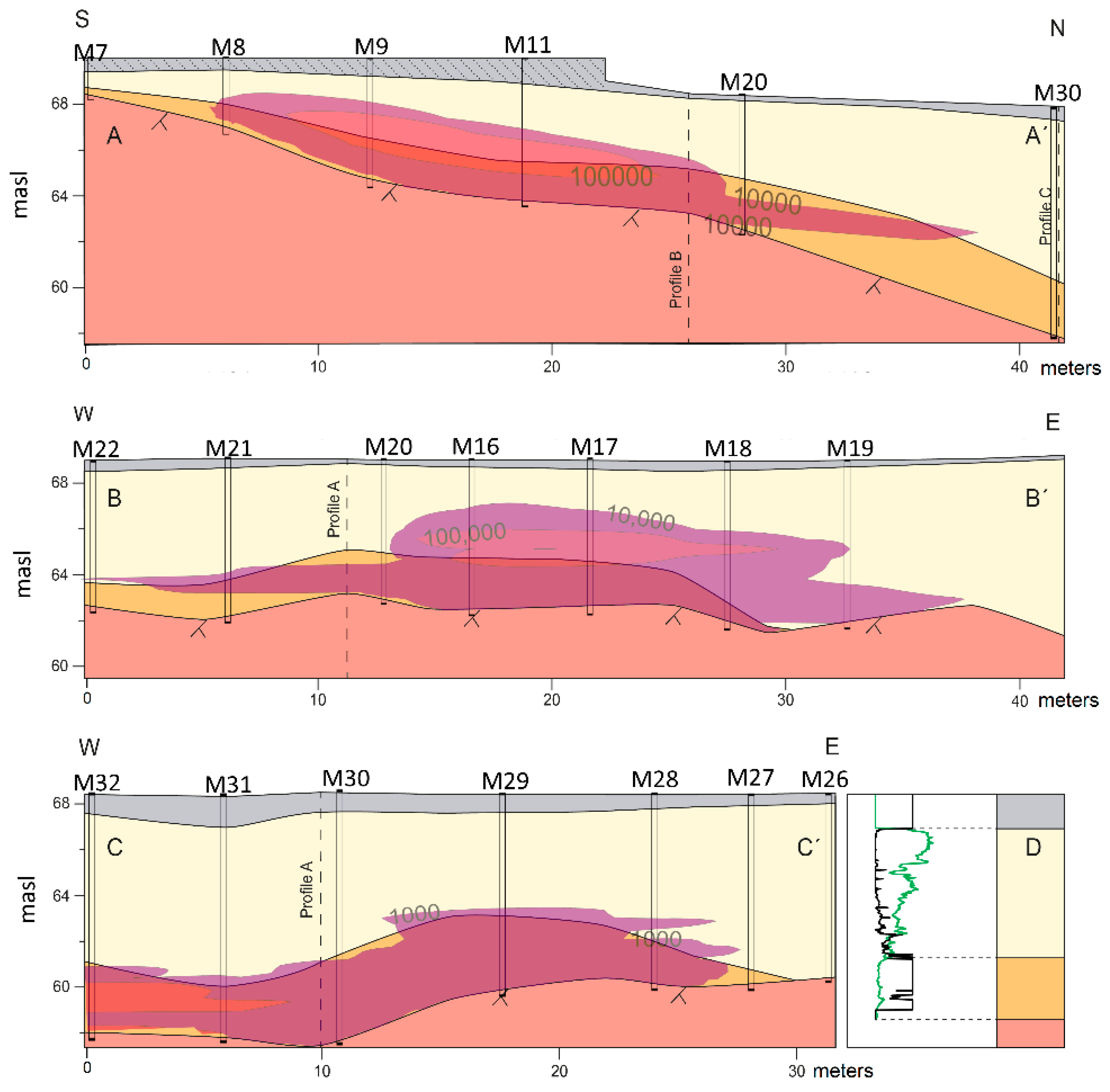
In the area of investigation, the depth to the bedrock varies between 2 to 10 m. The sediment overlying the bedrock is deposited in a fining upwards sequence. It consists of a meter of sand and gravel at the bottom, followed by clayey sandy silt, with sandy silty clay on top. On top of the sediment, about 1 m of fill material is present. Profiles describing the conceptual geology (
Figure 2, conceptual models, A–C) are elaborated based on interpretation of MIP results (
Figure 2, conceptual model, D) and borehole records. The interpreted results suggest, from the bedrock and up, a three-layer structure consisting of a coarse bottom unit, a “mixed fines” unit and a coarse gravel filling. The sedimentary units show a varying inner heterogeneity with lenses of both finer and coarser material occurring. The topography slopes gently towards NNW. The depth to the water table varies between 1.5 to 2 m below the ground surface and the groundwater flows from SE towards NW.
Between February 2nd and February 10th, 2017, the site was investigated using the MIP method [
27] and the raw data [
28] were further processed in this work. The plume was delineated to an area beneath the building and it extended outward beneath parts of the parking lot. The plume migrates towards NNW (
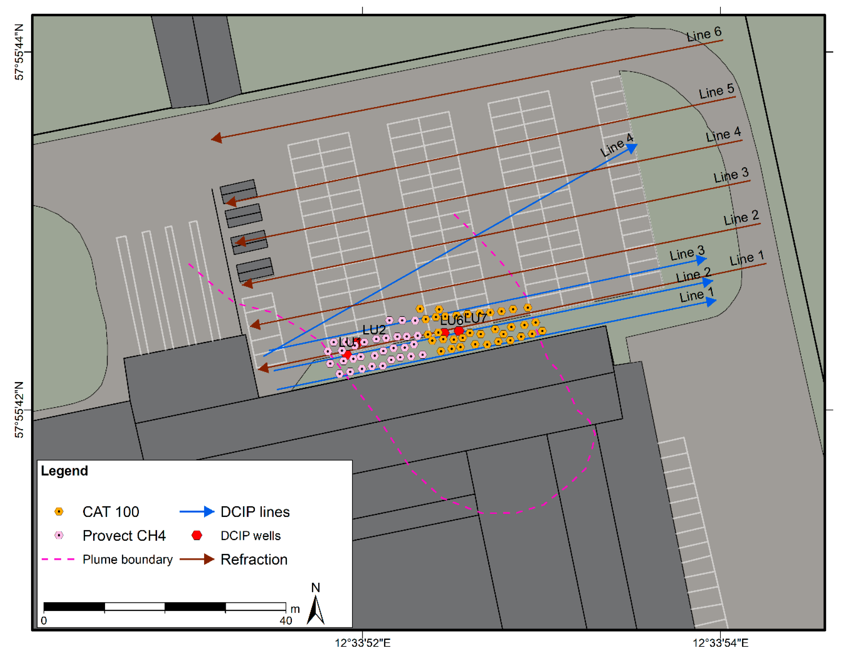
Figure 1), following the dip of the bedrock. In order to determine the best approach for treatment of the contamination and stop further spreading, a pilot in-situ remediation program was launched in November 2017, using a direct push injection method on the north side of the laundry building (
Figure 3). In order to evaluate the best approach for a future full-scale remediation scenario, two different remediating agents were injected into the plume at different locations, for comparison.
In injection area A (west side, see
Figure 3) Provectus ERD-CH4
TM substrate containing carbon source (electron donor) in the form of vegetable oils together with acids and a bacterial consortium (
Dehalococcoides mccartyi,
Desulfovibrio,
Desulfitobacterium and methanogenic archaea bacteria) was injected in two phases between the 7th and the 17th of November 2017, with a total of 32 points. In injection area B (east side, see
Figure 3) CAT100
TM-substrate containing granular activated carbon, zero-valent iron and Trap & Treat
® bacteria concentrate were injected, together with a methane inhibitor, between the 28
th and the 30
th of November 2017, in a total of 37 points. In both cases, the products were injected from a depth of 3 m and downward until reaching the top of the bedrock.
3. Method Description
3.1. Direct Current Resistivity and Time-Domain Induced Polarization
The DCIP method estimates the electrical resistivity and chargeability distribution in the subsurface [
29]. For the DCIP measurements, an ABEM Terrameter LS2 was used in the 100% duty-cycle mode [
30] and the full waveforms were recorded and processed to enhance the data quality [
31]. A pulse-length of 4 seconds was used averaging over four current pulses with alternate polarity to enhance the signal to noise ratio.
The measurements were focused on the contaminant source and plume area outside of the buildings where the pilot injection was planned to take place. Four DCIP surface lines (
Figure 3) with electrodes buried 40 cm into the ground were established to provide a permanent installation with a total of 64 stainless steel metal plate electrodes (10 × 10 cm) for each line in the DCIP monitoring system. The spacing between the electrodes is 1 m; however, the first four electrodes (except Line 4) and the last nine electrodes (all lines) are separated by 2 m to increase the depth of investigation. A multiple gradient array measurement sequence was used for the measurements [
32].
The processed data were inverted for the resistivity and integral chargeability of the ground using Res2dinvx64 (Geotomo Software, version 4.08). The grid refinement (horizontal model cell size of half the electrode spacing) and L1-norm (robust) inversion options were used, where the latter is better at handling strong contrast as well as noise in the data compared to least-squares (L2 norm) inversion. For the time-lapse inversion the smoothness constrained time-lapse inversion was used [
33] and the data sets shortly after the injection period were inverted against the baseline which was measured one week prior to the injection.
Furthermore, four boreholes with stainless steel ring electrodes were deployed, two in each injection area, to be used as pairs for cross-hole tomography. The separation of the wells was 2.7 m in injection area A, 2.5 m in injection area B and the electrodes were installed every 0.25 cm in each well up to the maximum depth. For the measurement sequence, the dipole-dipole array, containing a mixed set of inline and cross-borehole measurements, was used. The data were inverted using the DC2DPRO [
34,
35] software (version 1.01) using the least-squares inversion and the L1-norm error minimization option.
3.2. Seismic Refraction
Seismic refraction was used as a help to delineate depth to bedrock, as it provides continuous data over the area as opposed to borehole and MIP data, which offer only low spatial coverage. The seismic refraction method estimates the velocity with which the generated elastic wave (P-wave) propagates in the subsurface [
36]. The data were collected with a Geometrics StrataVisor paired with a Geometrics Geode recorder to increase the number of channels. Vertical component 4.5 kHz geophones, where used, were attached to a land streamer cable. An accelerated weight drop, mounted on a car, was used as a source. In total six parallel two-dimensional (2D) lines with 70 receivers were collected covering the parking lot area (
Figure 3). The spacing between the geophones was 1.25 m and the shots were fired between every 7,8 geophones. An offset shot was fired where sufficient space was available.
The first arrival events were picked for every line and then a 2D tomography was performed to obtain the distribution of P-wave velocities in the subsurface. The data was processed and inverted using the software Reflexw (Sandmeier Geophysical Research, version 8.5) with a curved ray-tracing model in a finite difference approximation.
4. Baseline Survey Results
4.1. Seismic Refraction Survey
Seismic refraction was used to investigate the depth to bedrock in the area around the parking lot, which is a downgradient of the contaminated source zone. The first seismic refraction line is not included in the results because the first arrivals were inconsistent due to the close proximity to the building. This could be due to reflected waves from the building’s foundations that reach the receivers faster than the refracted wave from the bedrock, providing a false image of the subsurface.
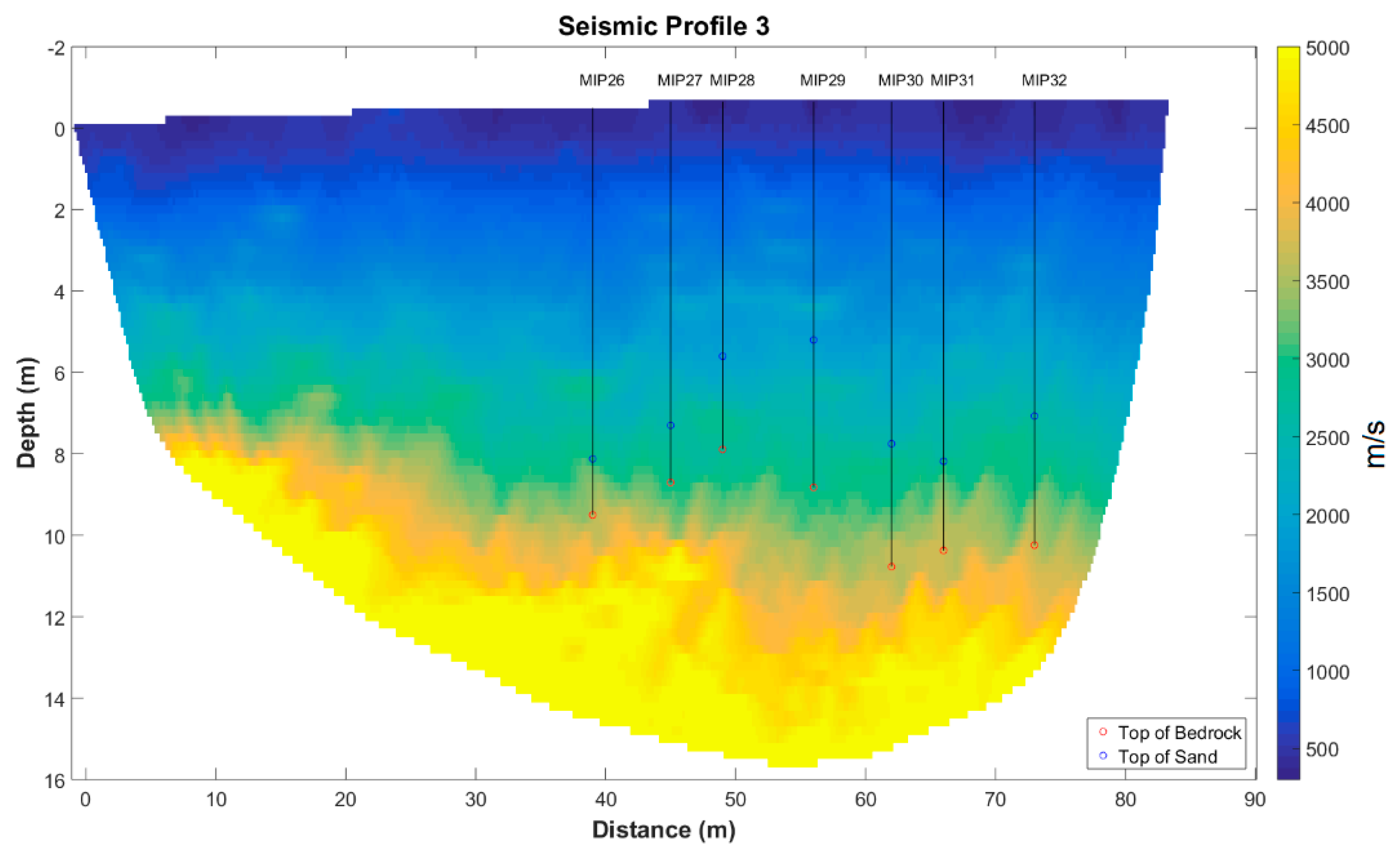
The interface between the sediments and the bedrock was expected to be identified by a sharp contrast in the inverted model. Furthermore, since we have information about the depth to bedrock from a different method, the direct push drilling, which was done in conjunction with the MIP soundings, we used the result from the SeismicLine3 (
Figure 4) to identify a velocity which represents the interface between the soft-sediments (low velocities) and the bedrock (higher velocities). The SeismicLine3 was chosen because it overlaps with more drill points in compared to the other lines. Based on the above, the velocity of 3500 m/s was chosen to represent the interface between the bedrock and the sediments.
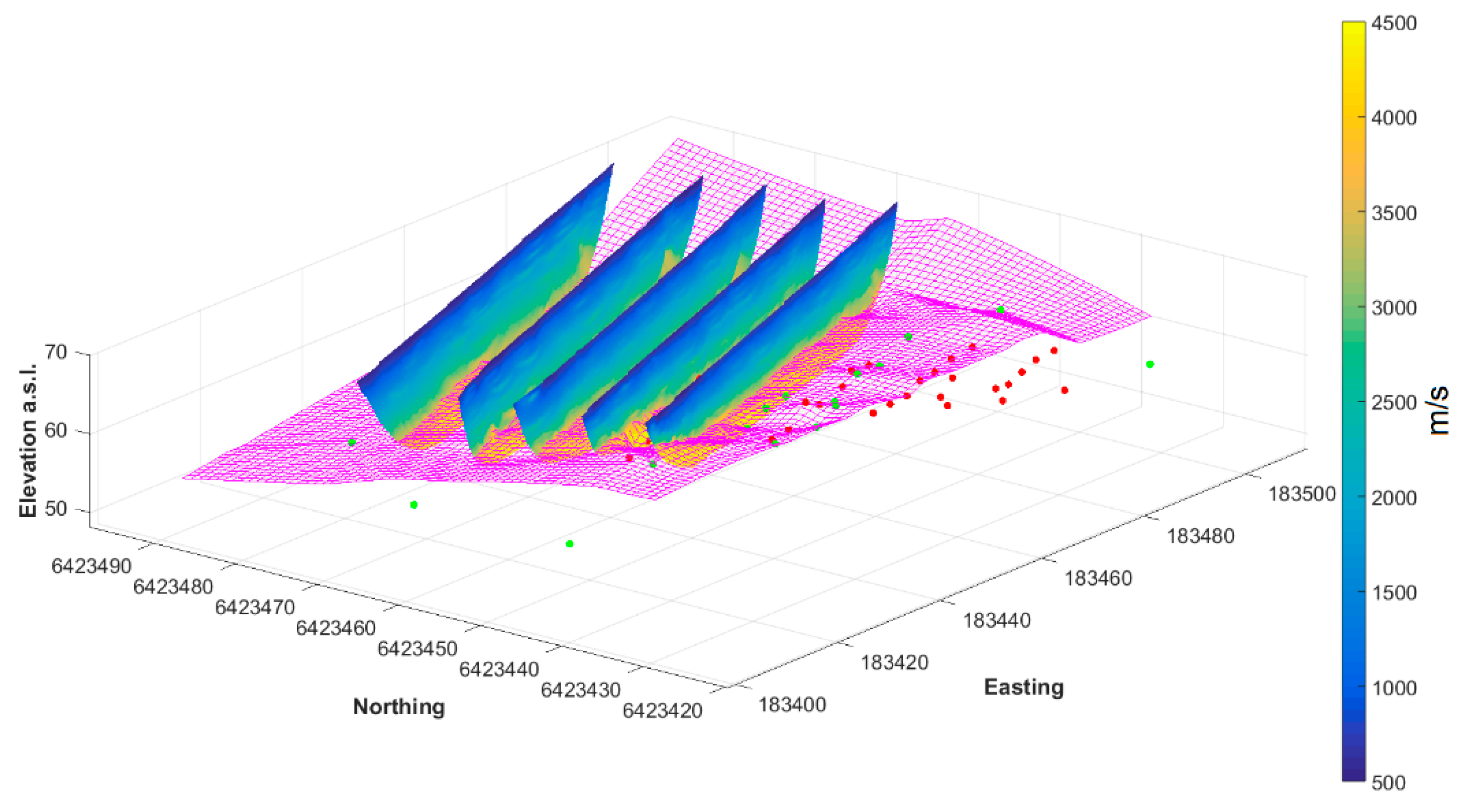
The results for all seismic refractions were plotted in a three-dimensional (3D) ‘fence’ diagram (
Figure 5). We used the of 3500 m/s velocity to fit a surface within the different tomography lines to acquire pseudo-3D representation of the bedrock surface, using linear interpolation.
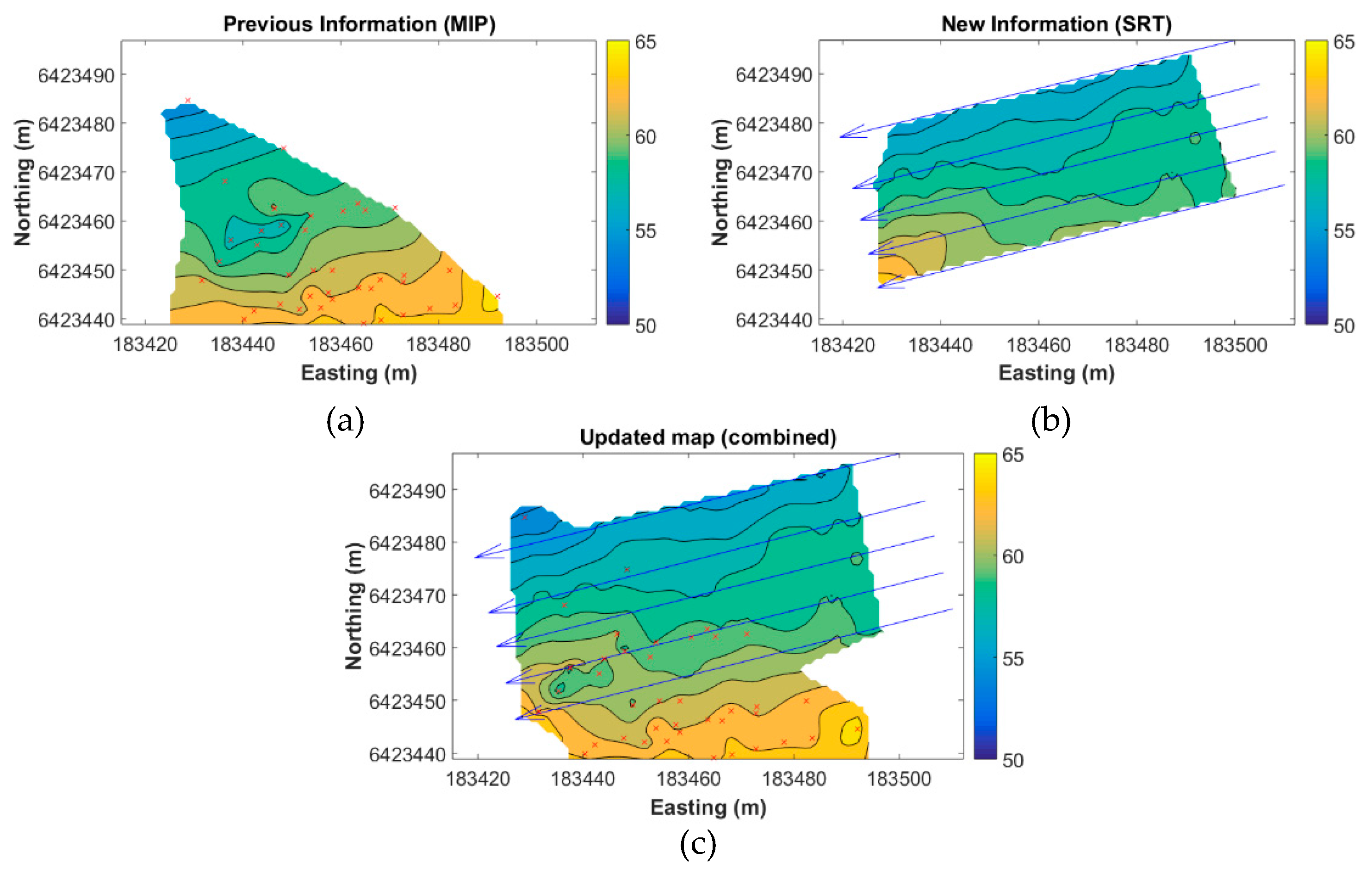
Finally, we exported the 3D surface acquired with the methodology described above and we used it to ‘expand’ the previously known depth to bedrock, based on the limited point information from the drillings and the MIP soundings (
Figure 1).
Figure 6 illustrates the depth to bedrock results that we acquired using the above methodology.
4.2. Direct Current Resistivity and Time-Domain Induced Polarization
The baseline resistivity and induced polarization data were collected using the autonomous system before any injections were performed. The data were collected to understand the geophysical signature of the geology and the contaminant prior to the injection of the fluids. Furthermore, the baseline data was also to estimate the signal to noise ratio and to identify buried infrastructure that could cause issues in the interpretation of the results.
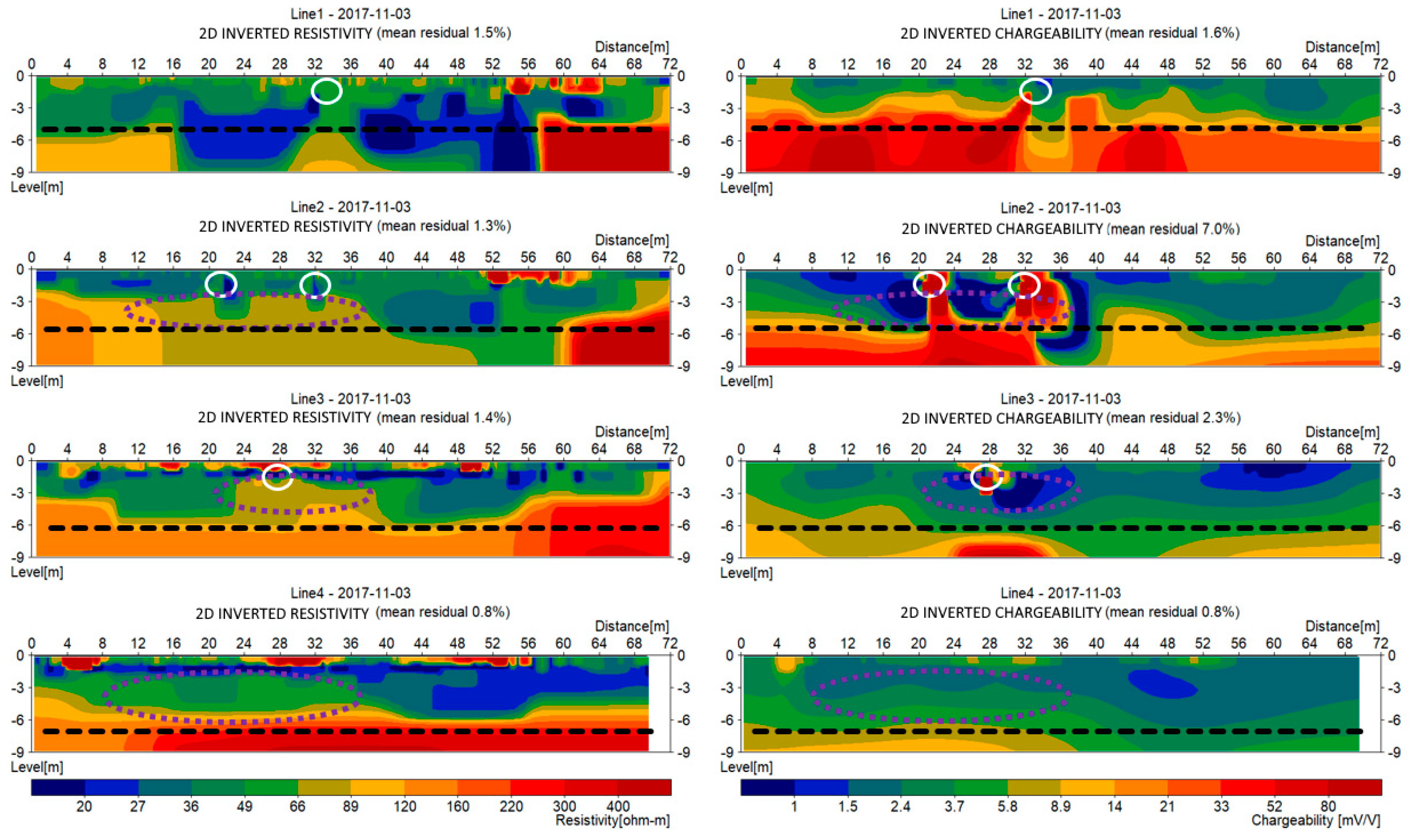
The data quality was very good, for both resistivity and chargeability data, based on the repeatability of the measurements (stacking), the low number of outliers (measurements that differ from their neighboring) and the regular shape of the IP decay curves. Furthermore, the residuals acquired from the inversions were similarly low (
Figure 7), as they were expected to be.
Firstly, the results appear to show a strong ‘3D-effect’ that affects the lines closer to the building, mainly the first line, which is judged to be caused by the foundations of the building (see
Figure 7). For the first three lines that run parallel to the building for most part, the edge of the building is marked. Furthermore, low resistivity and high chargeability responses (
Figure 8) can be seen in the first three lines and they coincide with known buried infrastructure objects such as groundwater/stormwater pipes and power cables, which most likely cause the anomalies (
Figure 7).
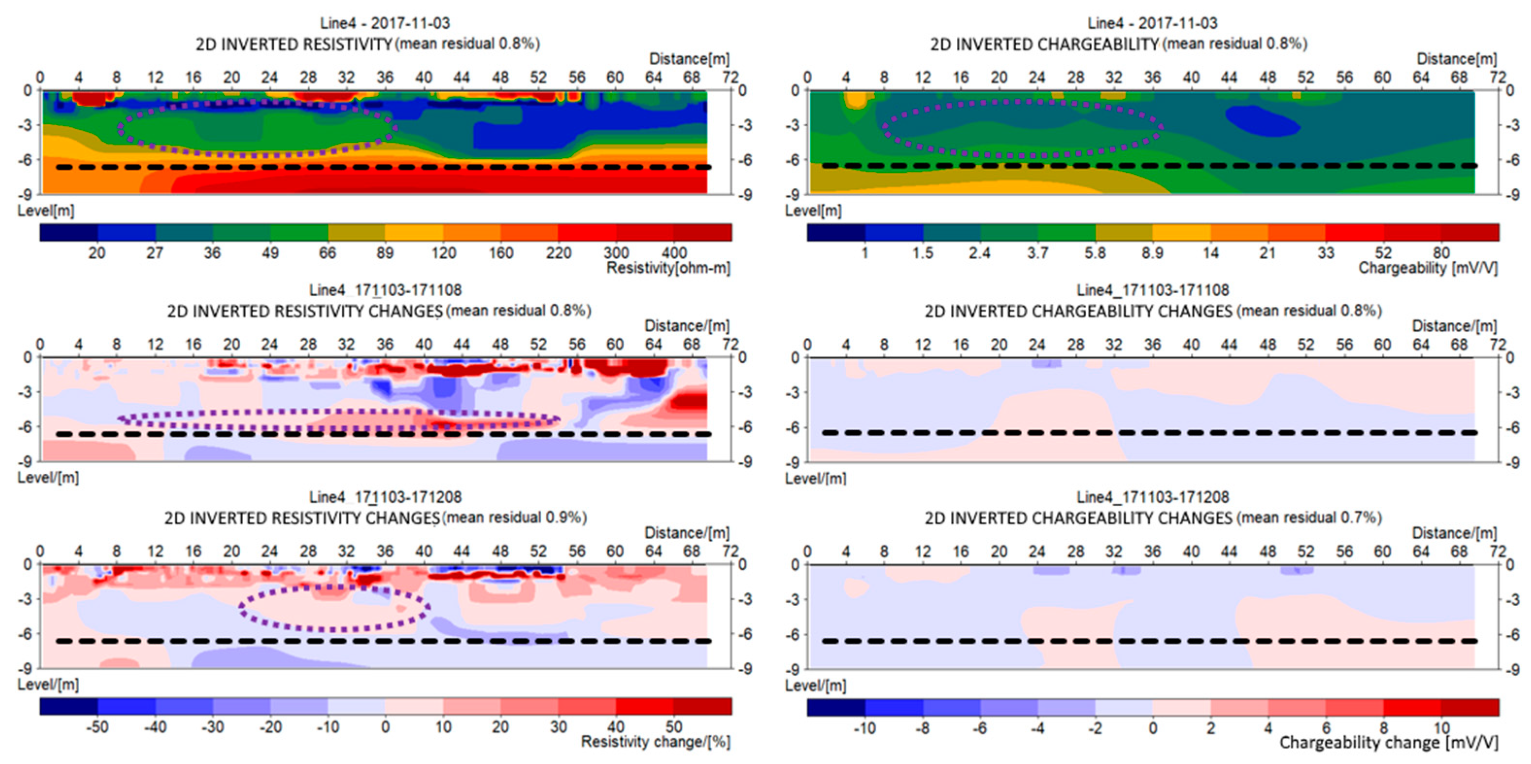
The resistivity results from Line 4 (
Figure 7) illustrate a layered stratigraphy where a high resistivity layer appears at the depth of 7 m and below, and this is interpreted as the granite bedrock. On top of that, there is a layer with significantly lower resistivities, which is interpreted as the quaternary sediments on top of the bedrock. There is a thin top layer of higher resistivity that corresponds to fill material that forms the base of the parking lot, underlain by a thin, low resistive layer that might be caused by a higher content of fines in the sediments. Below that, the resistivity of the sediments does not change so much with depth until the bedrock is reached, but it changes laterally. This can be seen at a distance interval of 23 to 38 m from the beginning of Line 3 (WSW), where the resistivity is significantly higher from around 2 m depth to the bedrock level, namely around 80 Ωm instead of below 50 Ωm as in the surrounding parts. Similarly, for Line 4, the resistivity changes from around 50 Ωm to below 30 Ωm at the distance of 35 m from the beginning of the line. A similar pattern can be observed to some extent from Line 2; however, the pattern becomes less visible the closer to the building the line is situated, making it very difficult to be distinguished in the first line.
The chargeability results from Line 4 (
Figure 7) illustrate a rise in the signal at a depth of 6–8 m which can partly be observed in Line 3 and Line 2, and maybe at an even higher magnitude. The response appears to be linked with the sand layer, where most of the contaminant degradation has been observed via the MIP soundings. Unfortunately, the signal is masked in the lines closer to the building due to the very strong shallow anomalies (
Figure 7) coming from the buried infrastructure and building foundation. The first line suffers the most, making it very hard to distinguish the same pattern due to the high magnitude of the shallow anomalies.
4.3. Cross-Hole Electrical Tomography
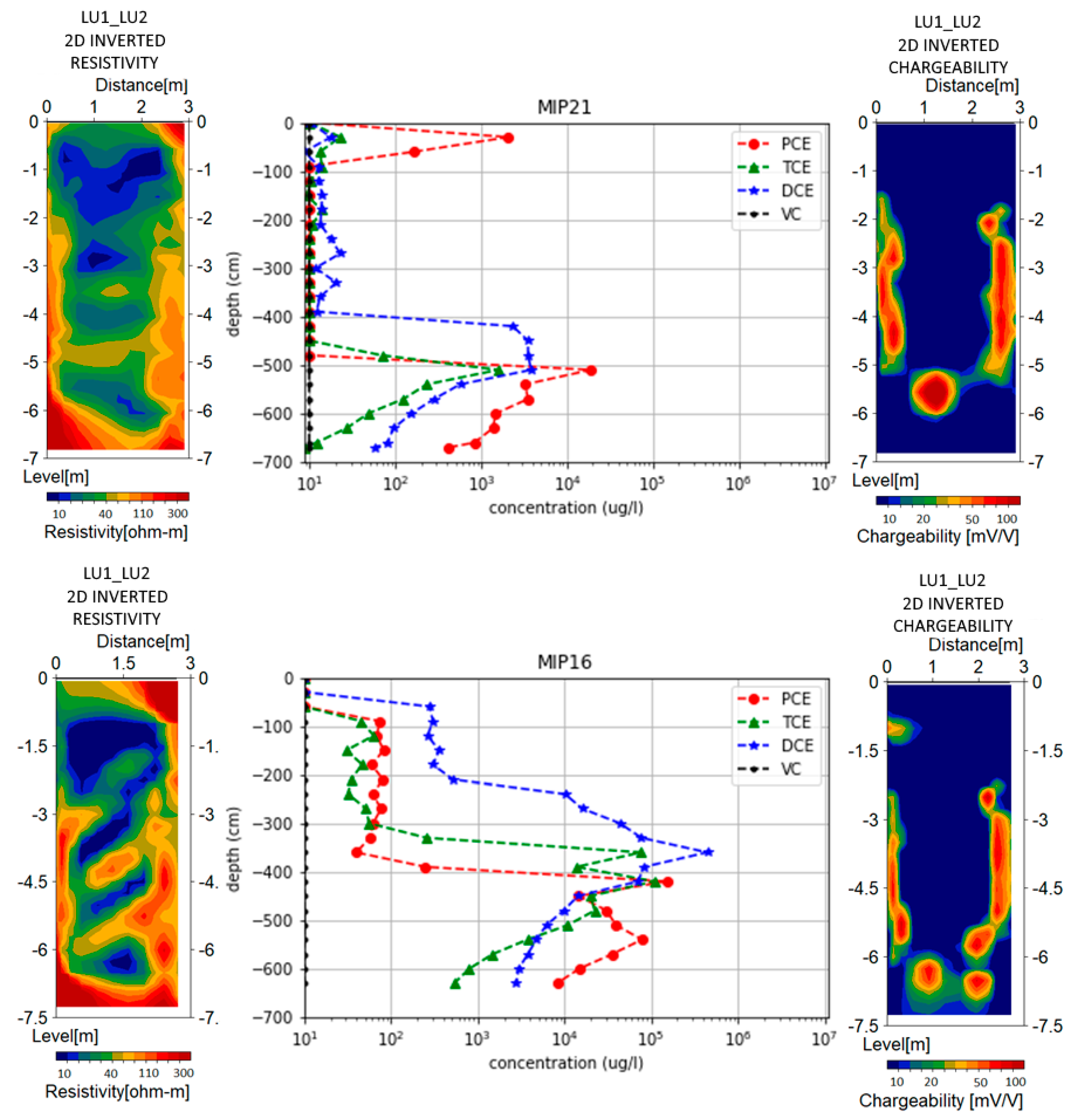
The resistivity results from the two cross-hole tomographies (
Figure 8) show a high resistivity response (300 Ωm) in close proximity to the well pipe, where the same resistive response appears to have high chargeability values (>100 mV/V) in the chargeability sections.
The area between the two wells appears with a low resistivity response (~10 Ωm) down to the depth of about 2 m with very low chargeabilities. Below a depth of 2 m, the resistivity shows a significant range (10–100 Ωm) where the chargeability is very low (<10 mV/V). At a depth of about 6 m at the area between the wells, there is an anomaly in the chargeability response in the range of 80–120 mV/V.
The MIP soundings 21 and 16 (
Figure 1) are in very close proximity of the cross-hole tomographies LU1_LU2 and LU6_LU7 (
Figure 3), respectively. The MIP soundings show a strong increase in the concentrations of the contaminant (PCE) and its degradations products (TCE, DCE and VC) (
Figure 8) from the depth of approximately 5 m and below.
5. Short-Term Monitoring Time-Lapse Results
The resistivity and chargeability data collected during the month the injections took place and short after were inverted and analyzed to identify spatial and temporal changes in the subsurface. Those changes should, at least partly, correspond to the effects of the injections in the ground and are expected to be rapid due to the nature of the direct push injection method used.
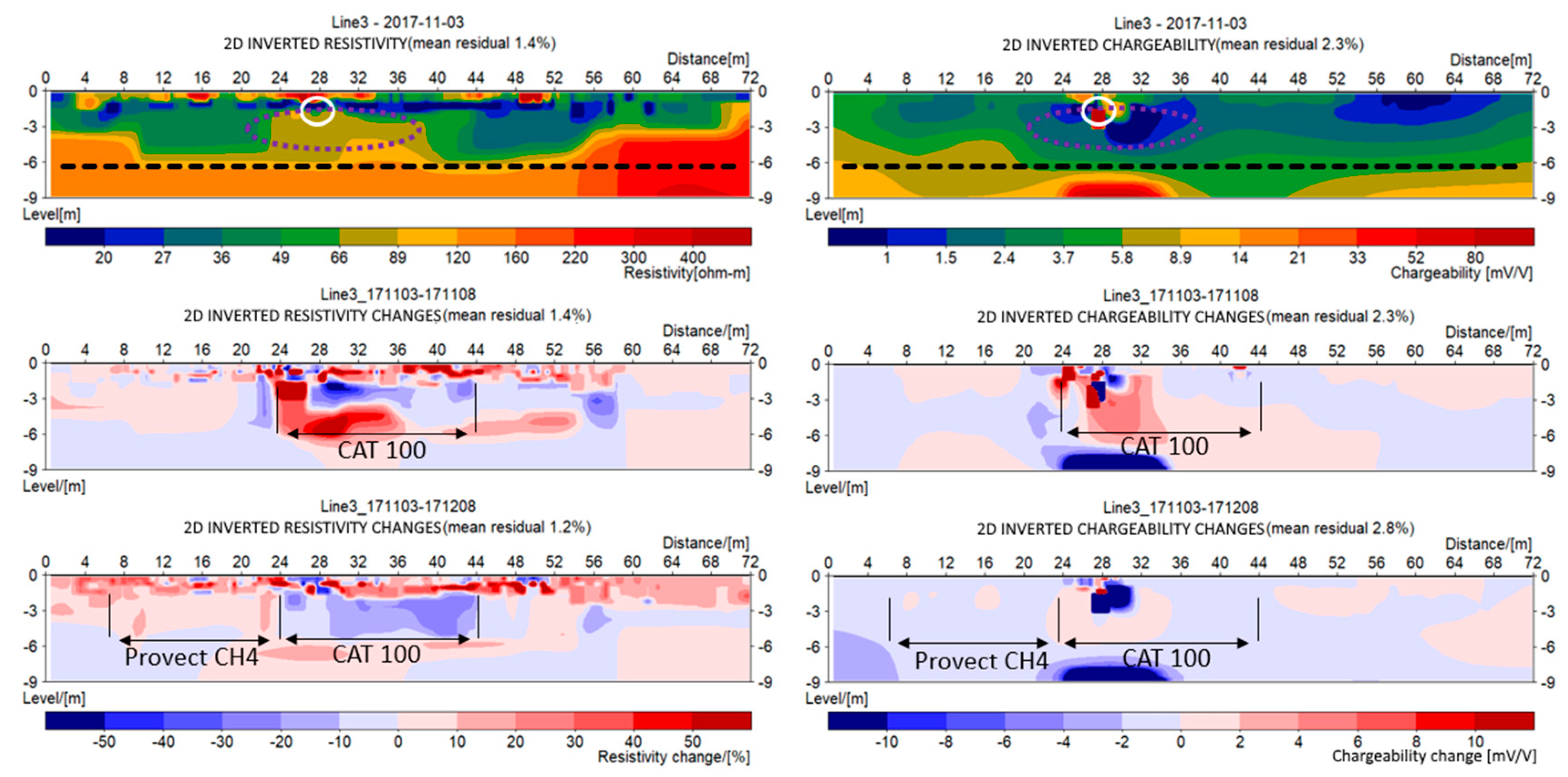
The results from the time-lapse inversion of Line 3, which crosses the area where the fluids were injected (
Figure 9), identify changes within the area of the injected products with an increased resistivity at the boundaries of the injection area. The changes in the resistivity following the injection of CAT100
TM (East, see
Figure 3) shows zones of increase as well as decrease in resistivity over the area during the injection of the product (
Figure 9 middle-left) where two weeks after the injection the same area appears with a decrease in the resistivity (
Figure 9 bottom-left) in comparison with the baseline survey. On the other hand, the area where the Provectus ERD-CH4
TM was injected (West, see
Figure 3) shows an increase in resistivity with distinct boundaries which corresponds to the injected volume (
Figure 9 bottom-left). The temporal changes in chargeability (
Figure 9 right) are rather small and are mainly around the pipe buried at 20 m from the start of the DCIP-line, either due to the more permeable area surrounding the pipe being filled up with injection liquids or due to artifacts introduced by the time-lapse inversion algorithm.
The temporal changes seen from Line 4, which is located outside the injection area (
Figure 3) show an increase in resistivity at the depth of 6–7 m (
Figure 10 middle-left), which coincides with the coarse (sand and gravel) layer that appears to be present in the area at that depth. The hydraulic conductivity of the coarse layer should be higher than the upper (clay) and lower (bedrock) geological units; therefore, one possible interpretation is that the injection fluids, most likely the CAT100™, show up due to flushing through the coarse-grained unit and into this down gradient area. The temporal changes in the chargeability are very low, meaning that there is no direct effect in the chargeability signature of the subsurface due to the injection, at least not in the time-step following the injections. The very small changes also strengthen the previous observation that the changes in the chargeability in Line 3 could be due to artifacts of the time-lapse inversion caused by the strong responses from the buried infrastructure.
6. Discussion
The contaminant is heavier than water and would, therefore, gravitationally sink in the ground, until it reaches an impermeable layer, which, in our study area, is probably the crystalline bedrock. Thus, it is imperative to know the boundaries of the bedrock interface. The results from the seismic refraction tomography indicate that the bedrock is dipping towards north-northwest, which, in combination with the groundwater flow, explains the migration of the PCE that led to the formation of the plume as showed from the MIP-soundings (
Figure 2). Furthermore, we utilize the seismic results to extrapolate the previous knowledge about the sediment-bedrock interface to investigate the possibility of the PCE to migrate in different directions. Based on our conceptual model for the area and the results from the geophysics, a scenario with spreading in other directions is highly unlikely, because neither the bedrock interface slope nor the groundwater flow would contribute to that. On the other hand, if the bedrock is fractured, it could be possible for the contaminant to migrate deeper into the bedrock; however, there is no such indication of that from the data collected in this work. This scenario needs to be carefully re-evaluated in the future.
The rather limited depression in the bedrock (
Figure 6a), which was identified by the MIP soundings MIP31, MIP32, MIP33 [
28] is not visible in the seismic refraction tomography. This is due to a limitation of the refraction seismic method, which, in this case, is unable to resolve small scale variations in the bedrock interface, because the first arrivals are not coming from the vertical direction but from the sides of the narrow depression. Therefore, the updated map for the depth to bedrock combines the information from the drillings (ground-truth) with the information from the geophysics. This is done to generate the depth to bedrock map (
Figure 6c) that better represents the area of investigation.
The results from the resistivity Line 4 are in good agreement with the conceptual model and the seismic survey, where the MIP soundings also indicate an interesting anomaly in the area where the contaminant has higher concentrations. The contaminant appears in the geophysical section as an increase in the resistivity, which is supported by previous studies of DNAPL contaminated sites [
4]. The results from the resistivity Line 3 shows some influence from the infrastructure, mainly the buried objects (power cables, water pipes etc.) and the foundation of the building. However, the increase of the resistivity response is in good correlation with the information from the MIP soundings and the conceptual model. The pattern is similar with the one observed in Line 4, which is interpreted as the geophysical signal from the contaminant.
The model that was proposed by Johansson [
4] describes a rise in the chargeability due to the degradation products of PCE (TCE, DCE, VC and Cl
-). We can identify an increase in the chargeability in the surface layouts that are not affected by the infrastructure (Line 3 and Line 4). Unfortunately, the infrastructure increases the complexity in the chargeability signal close to the building because the buried objects (mainly metal pipes) have high responses, which masks the expected lower responses coming from the degradation products of the contaminant.
The results from the cross-borehole tomography (
Figure 8) are very important in order to extract more detailed information about the subsurface over a smaller area. The electrodes are placed in the ground through drilling; therefore, the resolution is not reduced with depth as is the case with the surface layouts. The resistivity results (
Figure 7) indicate that the subsurface is not as homogeneous as previously described by the resistivity results of Line 3 and Line 4. The resistivity in the upper clay layer varies significantly, which could be explained by the presence of several silt and/or sand lenses in the clay, which is also verified by the drilling and MIP soundings. The results from the chargeability illustrate a strong borehole effect from the filling material around the well, which is bentonite pellets down to approximately the last meter and a half where it is sand (well filter). Of great importance is the clear anomaly of a high chargeability response at the bottom levels of the boreholes, which is depth-wise in excellent correlation with the contaminant and its degradation products measured with the MIP method (
Figure 8).
The temporal changes observed in Line 4 show no direct effect of the injection products on the chargeability signature of the subsurface, at least for the period right after the injections took place. The temperature of the injection fluids can partly explain the increase in the resistivity because the fluids are expected to be colder than the groundwater, since they were stored in the parking lot area during the cold winter where the temperature was close to 0 °C. The resistivity changes in Line 3 are very promising for using the method in order to identify injection fluids; however, more precise work needs to be done in order to extract quantitative results of the fluid distribution in the subsurface. The temporal resistivity changes, which correspond to the coarse layer present at Line 4, suggest that the injection fluids may have been flushed through the high hydraulic permeability media, the sand and gravel, in the direction down gradient of the injection area. The value of the injection fluids can be questioned if injected directly into high hydraulic permeability media, and this should be carefully considered, to avoid that the fluids flushes away from the area of interest.
The composition of the two consortiums differs significantly; the CAT100™ (east) contains iron particles to enhance the degradation process, while the Provectus™ (west) is essentially a cocktail of microbes that will actively feed from the contaminant reducing its concentration. Therefore, it is expected that the geophysical response from the two consortiums will be different as we can observe looking at the time-lapse results from Line 3 (
Figure 9) and Line 4 (
Figure 10).
7. Conclusions/Future Work
In this work, we have used seismic refraction, direct current and time-domain induced polarization tomography to investigate a site contaminated by chlorinated hydrocarbons. Geophysical data were used to expand previous knowledge of the area based on direct push drillings, with the membrane interface probe (MIP) sounding method.
The results from the MIP method were analyzed to create a simplified conceptual model for the area of interest and the geophysical data were used to expand that model. The formation of the DNAPL plume can be explained by the dipping of the bedrock (impermeable layer) and the ground water flow. Based on the bedrock topography and the groundwater flow direction we do not expect that the contaminant would have migrated in different paths, apart from possibly into bedrock fractures beneath the bedrock surface.
The resistivity results can identify the plume boundaries due to the increase in resistivity, whereas results from the chargeability can verify the presence of degradation products. A challenge arises in the interpretation of the results, especially the chargeability, in areas where the buried infrastructure generates strong responses, masking the much lower responses coming from the contamination. In such cases, it is important to have good quality borehole data, and to acquire data that would be less influenced by the infrastructure.
The time-domain resistivity and induced polarization results from Line 3, Line 4 and the cross-hole tomography appear to be very promising for the monitoring of the pilot test launched in late 2017. The method can provide qualitative information about the contaminant and the degradation products since the contaminant can be identified in the baseline survey. Therefore, the monitoring is expected to show promising results, since we can already observe changes, for the understanding of the impacts of in-situ remediation of chlorinated solvents as well as to pinpoint where actual samples need to be taken to verify changes in the underground.
Author Contributions
Conceptualization, A.N.; Data curation, A.N.; Formal analysis, A.N., T.D. and M.R.; Funding acquisition, T.D. and C.S.; Investigation, A.N., T.D. and M.R.; Methodology, A.N., T.D. and M.R.; Project administration, T.D. and C.S.; Visualization, A.N., M.R. and N.H.; Writing—original draft, A.N.; Writing—review and editing, A.N., T.D., M.R., N.H. and C.S.
Funding
This work has been carried out within the MIRACHL project (
http://mirachl.com/). Funding is provided by the Swedish Research Council Formas—The Swedish Research Council for Environment, Agricultural Sciences and Spatial Planning (ref. 2016-20099), SBUF—The Development Fund of the Swedish Construction Industry (ref. 13336), ÅForsk (ref. 14-332), SGU—Swedish Geological Survey, Sven Tyréns stiftelse, Västra Götalandsregionen and Lund University.
Acknowledgments
The authors would also like to acknowledge the valuable contribution of Stefano Fanari for assisting with the processing of the seismic refraction data, Ulf Winnberg for sharing the MIP raw data and Roger Wisén for his input while planning and carrying out the seismic refraction survey.
Conflicts of Interest
The authors declare no conflict of interest. The founding sponsors had no role in the design of the study; in the collection, analyses or interpretation of data; in the writing of the manuscript; and in the decision to publish the results.
Abbreviations
| MIP | membrane interface probe |
| DCIP | direct current time-domain induced polarization tomography |
| NAPLs | non-aqueous phase liquids |
| PCE | tetrachloroethylene |
| TCE | trichloroethene |
| DCE | dichloroethane |
| VC | vinyl chloride |
| DNAPLs | dense non-aqueous phase liquids |
| SGU | Swedish geological survey |
| SEPA | Swedish environmental protection agency |
| SRT | seismic refraction tomography |
References
- Swedish Environmental Protection Agency. Nationell Plan för Fördelning av Statliga Bidrag för Efterbehandling; Report 6617; Swedish Environmental Protection Agency: Stockholm, Sweden, 2014; Volume 30. (In Swedish) [Google Scholar]
- Lin, K.S.; Mdlovu, N.V.; Chen, C.Y.; Chiang, C.L.; Dehvari, K. Degradation of TCE, PCE, and 1,2–DCE DNAPLs in contaminated groundwater using polyethylenimine-modified zero-valent iron nanoparticles. J. Clean. Prod. 2018, 175, 456–466. [Google Scholar] [CrossRef]
- Scheffer, B.; van de Ven, E. Experiences of Perozone and C-Sparge at Two Former Dry Cleaner Sites in the Netherlands. Ozone Sci. Eng. 2010, 32, 130–136. [Google Scholar] [CrossRef]
- Johansson, S.; Fiandaca, G.; Dahlin, T. Influence of non-aqueous phase liquid configuration on induced polarization parameters: Conceptual models applied to a time-domain field case study. J. Appl. Geophys. 2015, 123, 295–309. [Google Scholar] [CrossRef]
- Flores Orozco, A.; Williams, K.H.; Kemna, A. Time-lapse spectral induced polarization imaging of stimulated uranium bioremediation. Surf. Geophys. 2013, 11, 531–544. [Google Scholar] [CrossRef]
- Bernstone, C.; Dahlin, T.; Ohlsson, T.; Hogland, W. DC-resistivity mapping of internal landfill structures: Two pre-excavation surveys. Environ. Geol. 2000, 39, 360–371. [Google Scholar] [CrossRef]
- Chambers, J.E.; Kuras, O.; Meldrum, P.I.; Ogilvy, R.D.; Hollands, J. Electrical resistivity tomography applied to geologic, hydrogeologic, and engineering investigations at a former waste-disposal site. Geophysics 2006, 71, B231–B239. [Google Scholar] [CrossRef]
- Gazoty, A.; Fiandaca, G.; Pedersen, J.; Auken, E.; Christiansen, A.V. Mapping of landfills using time-domain spectral induced polarization data: The Eskelund case study. Surf. Geophys. 2012, 10, 575–586. [Google Scholar] [CrossRef]
- Ustra, A.T.; Elis, V.R.; Mondelli, G.; Zuquette, L.V.; Giacheti, H.L. Case study: A 3D resistivity and induced polarization imaging from downstream a waste disposal site in Brazil. Environ. Earth Sci. 2012, 66, 763–772. [Google Scholar] [CrossRef]
- Power, C.; Tsourlos, P.; Ramasamy, M.; Nivorlis, A.; Mkandawire, M. Combined DC resistivity and induced polarization (DC-IP) for mapping the internal composition of a mine waste rock pile in Nova Scotia, Canada. J. Appl. Geophys. 2018, 150, 40–51. [Google Scholar] [CrossRef]
- Ntarlagiannis, D.; Robinson, J.; Soupios, P.; Slater, L. Field-scale electrical geophysics over an olive oil mill waste deposition site: Evaluating the information content of resistivity versus induced polarization (IP) images for delineating the spatial extent of organic contamination. J. Appl. Geophys. 2016, 135, 418–426. [Google Scholar] [CrossRef]
- Wemegah, D.D.; Fiandaca, G.; Auken, E.; Menyeh, A.; Danuor, S.K. Spectral time-domain induced polarisation and magnetic surveying—An efficient tool for characterisation of solid waste deposits in developing countries. Surf. Geophys. 2017, 15, 75–84. [Google Scholar] [CrossRef]
- Park, S.; Yi, M.-J.; Kim, J.-H.; Shin, S.W. Electrical resistivity imaging (ERI) monitoring for groundwater contamination in an uncontrolled landfill, South Korea. J. Appl. Geophys. 2016, 135, 1–7. [Google Scholar] [CrossRef]
- Leroux, V.; Dahlin, T.; Rosqvist, H. Time-domain IP and Resistivity Sections Measured at Four Landfills with Different Contents. In Proceedings of the Near Surface 2010—16th Europe Meeting of Environment and Engineering Geophysics (EAGE), Zurich, Switzerland, 6–8 September 2010. [Google Scholar]
- Kuras, O.; Wilkinson, P.B.; Meldrum, P.I.; Oxby, L.S.; Uhlemann, S.; Chambers, J.E.; Binley, A.; Graham, J.; Smith, N.T.; Atherton, N. Geoelectrical monitoring of simulated subsurface leakage to support high-hazard nuclear decommissioning at the Sellafield Site, UK. Sci. Total Environ. 2016, 566–567, 350–359. [Google Scholar] [CrossRef] [PubMed]
- Rosqvist, H.; Leroux, V.; Dahlin, T.; Svensson, M.; Lindsjö, M.; Månsson, C.-H.; Johansson, S. Mapping landfill gas migration using resistivity monitoring. Proc. Inst. Civ. Eng.—Waste Resour. Manag. 2011, 164, 3–15. [Google Scholar] [CrossRef]
- Steelman, C.M.; Klazinga, D.R.; Cahill, A.G.; Endres, A.L.; Parker, B.L. Monitoring the evolution and migration of a methane gas plume in an unconfined sandy aquifer using time-lapse GPR and ERT. J. Contam. Hydrol. 2017, 205, 12–24. [Google Scholar] [CrossRef]
- Flores Orozco, A.; Kemna, A.; Oberdörster, C.; Zschornack, L.; Leven, C.; Dietrich, P.; Weiss, H. Delineation of subsurface hydrocarbon contamination at a former hydrogenation plant using spectral induced polarization imaging. J. Contam. Hydrol. 2012, 136–137, 131–144. [Google Scholar] [CrossRef]
- Power, C.; Gerhard, J.I.; Karaoulis, M.; Tsourlos, P.; Giannopoulos, A. Evaluating four-dimensional time-lapse electrical resistivity tomography for monitoring DNAPL source zone remediation. J. Contam. Hydrol. 2014, 162–163, 27–46. [Google Scholar] [CrossRef]
- Johansson, S.; Sparrenbom, C.; Fiandaca, G.; Lindskog, A.; Olsson, P.-I.; Dahlin, T.; Rosqvist, H. Investigations of a Cretaceous limestone with spectral induced polarization and scanning electron microscopy. Geophys. J. Int. 2017, 208, 954–972. [Google Scholar] [CrossRef]
- Simyrdanis, K.; Papadopoulos, N.; Soupios, P.; Kirkou, S.; Tsourlos, P. Characterization and monitoring of subsurface contamination from Olive Oil Mills’ waste waters using Electrical Resistivity Tomography. Sci. Total Environ. 2018, 637–638, 991–1003. [Google Scholar] [CrossRef]
- Maurya, P.K.; Balbarini, N.; Møller, I.; Rønde, V.; Christiansen, A.V.; Bjerg, P.L.; Auken, E.; Fiandaca, G. Subsurface imaging of water electrical conductivity, hydraulic permeability and lithology at contaminated sites by induced polarization. Geophys. J. Int. 2018, 213, 770–785. [Google Scholar] [CrossRef]
- Sparrenbom, C.J.; Åkesson, S.; Johansson, S.; Hagerberg, D.; Dahlin, T. Investigation of chlorinated solvent pollution with resistivity and induced polarization. Sci. Total Environ. 2017, 575, 767–778. [Google Scholar] [CrossRef] [PubMed]
- Caterina, D.; Flores Orozco, A.; Nguyen, F. Long-term ERT monitoring of biogeochemical changes of an aged hydrocarbon contamination. J. Contam. Hydrol. 2017, 201, 19–29. [Google Scholar] [CrossRef] [PubMed]
- Flores Orozco, A.; Velimirovic, M.; Tosco, T.; Kemna, A.; Sapion, H.; Klaas, N.; Sethi, R.; Bastiaens, L. Monitoring the injection of microscale zerovalent iron particles for groundwater remediation by means of complex electrical conductivity imaging. Environ. Sci. Technol. 2015, 49, 5593–5600. [Google Scholar] [CrossRef] [PubMed]
- Göransson, M.; Bergström, U.; Shomali, H. Beskrivning till Bergkvalitetskartan Alingsås Kommun. Sveriges Geologiska Undersökning. 2007. Available online: http://resource.sgu.se/produkter/k/k68-beskrivning-bergkvalite.pdf (accessed on 20 February 2018).
- Balzarini, T.; Van Herreweghe, S. EnISSA campaign, WSP SVERIGE AB, Tvätterigatan 3, Alingsås (SE). Project reference: 17/171. 2017; unpublished work. [Google Scholar]
- Winnberg, U. (SGU, Stockholm, Sweden). Personal communication, 2018.
- Loke, M.H.; Chambers, J.E.; Rucker, D.F.; Kuras, O.; Wilkinson, P.B. Recent developments in the direct-current geoelectrical imaging method. J. Appl. Geophys. 2013, 95, 135–156. [Google Scholar] [CrossRef]
- Olsson, P.-I.; Dahlin, T.; Fiandaca, G.; Auken, E. Measuring time-domain spectral induced polarization in the on-time: Decreasing acquisition time and increasing signal-to-noise ratio. J. Appl. Geophys. 2015, 123, 316–321. [Google Scholar] [CrossRef]
- Olsson, P.-I.; Fiandaca, G.; Larsen, J.J.; Dahlin, T.; Auken, E. Doubling the spectrum of time-domain induced polarization by harmonic de-noising, drift correction, spike removal, tapered gating and data uncertainty estimation. Geophys. J. Int. 2016, 207, 774–784. [Google Scholar] [CrossRef]
- Dahlin, T.; Zhou, B. A numerical comparison of 2D resistivity imaging with 10 electrode arrays. Geophys. Prospect. 2004, 52, 379–398. [Google Scholar] [CrossRef]
- Loke, M.H.; Dahlin, T.; Rucker, D.F. Smoothness-constrained time-lapse inversion of data from 3D resistivity surveys. Surf. Geophys. 2014, 12, 5–24. [Google Scholar] [CrossRef]
- Yi, M.-J.; Kim, J.H.; Chung, S.-H. Enhancing the Resolving Power of Least-Squares Inversion with Active Constraint Balancing. Geophysics 2003, 68, 931–941. [Google Scholar] [CrossRef]
- Kim, J.H.; Supper, R.; Tsourlos, P.; Yi, M.-J. 4D Inversion of Resistivity Monitoring Data through Lp Norm Minimizations. Geophys. J. Int. 2013, 195, 1640–1656. [Google Scholar] [CrossRef]
- Sheehan, J.R.; Doll, W.E.; Mandell, W.A. An evaluation of methods and available software for seismic refraction tomography analysis. J. Environ. Eng. Geophys. 2005, 10, 21–34. [Google Scholar] [CrossRef]
© 2019 by the authors. Licensee MDPI, Basel, Switzerland. This article is an open access article distributed under the terms and conditions of the Creative Commons Attribution (CC BY) license (http://creativecommons.org/licenses/by/4.0/).

 ,
, 


