The Use of a Grid Structure for Reconstructing and Forecasting the Value of Real Estate in Selected Measurement Epochs

Abstract

The absence of sufficiently long time series of data relating to real estate prices in a selected location prevents accurate analyses and the development of precise forecasts that play an important role in a market economy. New methods and solutions are being sought to address this problem. This paper proposes an original method for reconstructing, forecasting and archiving data relating to real estate value. The proposed method involves a GRID (regular square nets) structure and it relies on the prices quoted in successive years (epochs) of measurement in a selected object. Irregularly distributed measurement data (real estate prices) acquired in successive years are transformed into a regular GRID structure to develop digital surface models that describe the distribution of data. The nodes of the GRID structure are described with the coefficients of an approximating polynomial to reconstruct and forecast real estate value in a specific location at any point in time. A GRID structure supports a comparison of changes in real estate value over time in a given node or group of nodes selected from successive measurement epochs. Individual coefficients of an approximating polynomial are generated, allocated to selected nodes, and automatically adapted to local changes in value. As a result, the observed changes can be described in a given period of time. Source data covering multiple epochs are replaced with a single file containing coefficients of approximating polynomials to reduce the size of the stored datasets and facilitate data management.

1. Introduction

Residential real estate plays an important role in the spatial structure of a town or a city, and it is an important element of the urban management system which considerably influences economic development, in particular decision-making processes. Housing constitutes a large subsector of the real estate market, and the majority of market transactions involve residential real estate. This segment of the real estate market is characterised by high levels of activity that are reflected in the number of conducted transactions. The demand for housing is affected by numerous factors, where residential needs play the key role. The supply of housing is determined by the existing resources and new development projects. The real estate market is a complex system that is characterised by broad spatial coverage, a large number of transactions, highly dynamic market phenomena, and large amounts of data. At the same time, the real estate market is highly diverse due to the location and physical attributes of real estate, political factors, information flow, macroeconomic and microeconomic factors, as well as global and national shocks. As a result, the real estate market is difficult to analyze [1,2,3,4]. The variability of prices over time and real estate values cannot be easily identified due to the low frequency of transactions in a specific location (the overall number of transactions is high, but the number of transactions in a specific location can be very low). Depending on the purpose of the analysis, real estate value can be determined in the past, present or future. The variability of real estate prices over time has been analyzed by numerous authors [5,6,7,8,9,10,11,12,13,14,15,16,17]. Such analyses involve time series methods, fuzzy logic methods, time trends, multiple regression, hedonistic regression, spatiotemporal forecasting, spatiotemporal autoregression, price modelling, and indicators of variation in real estate prices. The absence of sufficiently long time series of data relating to real estate prices in a selected location prevents accurate analyses and the development of precise forecasts that are important in a market economy. New methods and solutions are being sought to address this problem. In this study, the GRID method was used to prepare data for spatiotemporal analysis based on a complete network of nodes. The proposed approach supports the determination of time intervals at any point in the analyzed space (node) as well as the approximation of changes that occur over time in every epoch with the use of a polynomial with an automatically determined degree.

Spatial Information Systems (SIS) support the acquisition, collection, processing, and sharing of spatial and descriptive data relating to various objects [18,19,20,21,22,23]. Therefore, these systems are increasingly often used to perform operations where the location and identity of objects in a spatial frame of reference play the main role. Spatial information systems are commonly used to describe, analyze, explain, interpret, and predict different kinds of spatial phenomena [24,25,26]. Due to the growing demand for information, the applicability of modern SIS is determined mainly based on their ability to collect large amounts of data in the shortest possible time as well as their dynamic updating, processing and data-sharing capabilities. Various types of data change dynamically within a relatively short time. Such changes can be identified through multiple analyses of the data relating to the same area in successive measurement epochs. In this approach, the studied object (or economic and physical phenomena) is measured at different points in time, which leads to a rapid increase in the volume of the processed data. The above applies particularly to situations where various aspects of reality are measured (not only spatial coordinates of objects, but also their quality attributes), and analyses are conducted in real time [27,28]. Therefore, the requirements for SIS continue to increase with a growing volume of collected and processed data (especially data collected during several measurement epochs at various points in time). Data gathering methods and processing techniques have to evolve to meet those requirements.

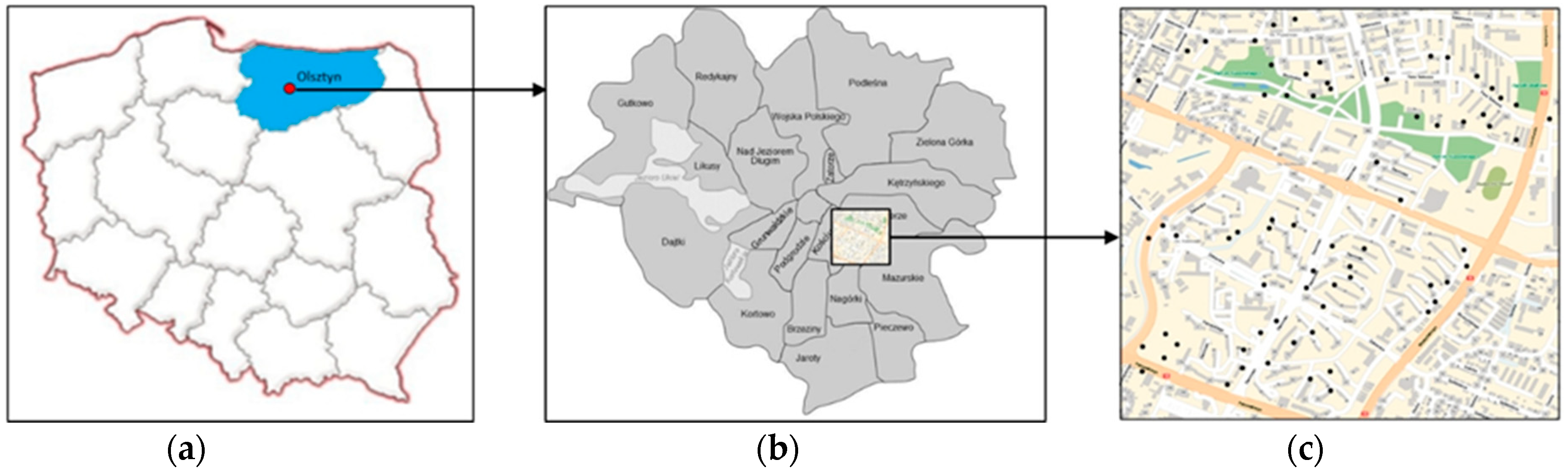
This paper proposes a method for reconstructing, forecasting and archiving data relating to the values of residential property in successive years of measurements in a selected object (measurement epochs which denote successive years of data registration). In this study, the term “reconstruction” denotes the search for missing data (in nodes or epochs) based on the values recorded in nodes or in the neighbouring epochs. “Measurement points” denote the geometric centre of a building where the analyzed transaction took place (Section 3.1). Modelling and calculations were performed with the use of dedicated software developed by the authors. In the proposed approach, one of the many interpolation methods was deployed to generate a GRID network and extract the values allocated to individual network nodes in successive measurement epochs.

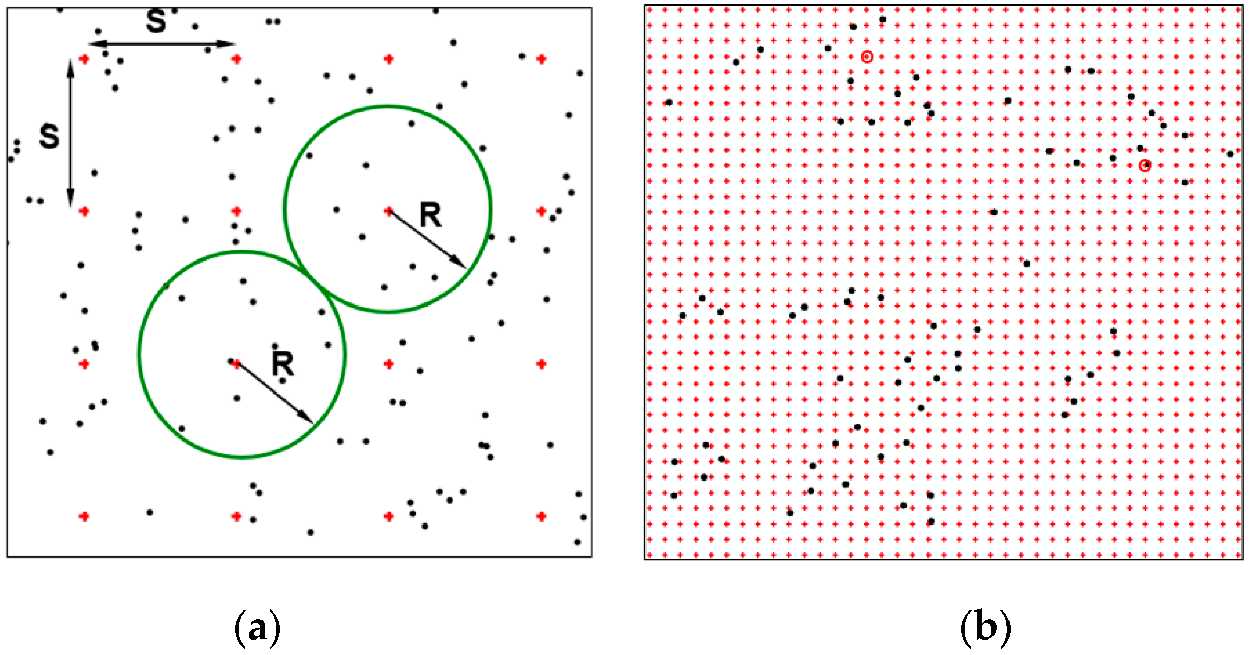
Irregularly distributed measurement data (real estate prices) acquired in successive years are transformed into a regular GRID structure to develop digital surface models. The models describe the distribution of prices in an object in each epoch. In the simplest terms, real estate prices constitute points whose spatial distribution can be interpolated. This approach is based on the assumption that space is continuous, and that real estate is an element of space; therefore, the surface of a variable (the price of real estate) is also continuous (in consequence, the value can be estimated at each point). A variable is also space-dependent (the value in a specific location is associated with the values in adjacent locations). The data (prices) which make up a time series are described by the coefficients of polynomials whose degree is determined automatically. The description of GRID nodes with the coefficients of approximating polynomials supports the reconstruction and prediction of real estate value at any point in time in the measurement epoch. As a result, the number of points stored in a database can be reduced without compromising the precision of spatial models generated in the process. The size of the datasets to be incorporated into SIS is optimized, and data are archived effectively, which considerably facilitates analysis.

The proposed method relies on GRID structures generated in successive measurement epochs to prepare data for time-series analysis. The data from each measurement epoch are used to generate a GRID structure with a complete network of nodes. This approach generates a full set of data in every epoch (node), which supports the determination of specific time intervals at every point in the analyzed space. Values that change over time are selected in each node (at the same point in each epoch), and they are approximated with the use of a polynomial with an automatically determined degree. The polynomial supports the description of changes over time with the use of coefficients that are allocated to each node. The data recorded in multiple measurement epochs are stored in a single file, which reduces the volume of the resulting dataset. The above improves the effectiveness of archiving operations, accelerates data exchange and facilitates resource management. In each node, the coefficients of approximating polynomials contain information about changes in real estate value, and they can also be used to generate surfaces that are allocated to a selected epoch and to reconstruct values at any point in time.

The coefficients of approximating polynomials are used to reconstruct the value of nodes with the same location (x, y) based on individually determined polynomials. This approach supports the reconstruction of the time series in each node. The coefficients are generated independently for each node in every epoch, and they are influenced by the degree of the polynomial describing changes in node values over time. The time interval between the reconstructed epochs can be freely set, which supports the determination of intermediate epochs. As a result, data can be reconstructed at any point in time without the need to archive the entire dataset, which reduces the volume of data required for the recreation of a complete GRID structure for a given point in time. The resulting database contains only the coefficients of approximating polynomials which describe changes in the examined phenomenon, which supports comprehensive analyses.

2. Materials and Methods

Subject Matter of the Study

The analyses were conducted based on the information about market transactions involving residential real estate (apartments). This approach was adopted due to a high number of transactions which formed a homogeneous dataset. The traded apartments were characterised by low levels of diversity (they were highly similar in terms of legal status, construction technology, year of construction—age of the buildings of 35–40 years, renovation and insulation standards, technical condition and wear, utility parameters—comparable usable floor area of 40 to 60 m², and dense development in a residential estate); therefore, the average price of a model apartment in a given location could be accurately determined.

The accumulated data cover 2005–2014, and they reflect the dynamics of changes on the market. The analyzed period covers the global financial crisis which affected the trends on local real estate markets. The proposed method was tested on the real estate prices quoted in different periods.

The proposed method is highly versatile and can be applied to any object. The studied objects were apartments in the residential estate of Pojezierze (Figure 1b) in the city of Olsztyn (Region of Warmia and Mazury, Poland) (Figure 1a) because the relevant data were widely available and the results could be verified. The spatial distribution of the buildings featuring apartments that were analyzed in each year is marked with points and presented in Figure 1c.

3. Results

3.1. Interpolation of Real Estate Prices with a GRID Structure

The data collected for each of the 10 measurement periods (successive years) were stored at one level in a database with three fields. Each record contained geographic coordinates (in the adopted frame of reference—WGS 84 Web Mercator) of the geometric centre of a building where the traded apartment was situated, and the average unit price (PLN/m²) in a given location. The data from each measurement set were marked with a rectangle (N: 53.763744–53.781306; E: 20.491453–20.510377) with an area of 2.3543 km² to produce equally-sized samples for analysis. Ten separate datasets covering the same area in each measurement epoch were created. Due to the specificity of the real estate market, apartments are geographically dispersed (Figure 1c). The location differed in subsequent measurement epochs. The resulting datasets describing the location and the prices of the examined apartments differed across years, which complicated the analysis.

The volume of data and the location of examined apartments also differed in successive measurement epochs (year-volume of data): 2005-72; 2006-54; 2007-71; 2008-75; 2009-64; 2010-72; 2011-67; 201-70; 201-85; 201-72.

The modelling of continuous phenomena requires the reconstruction and forecasting of values at any point in the generated object. The measurement points registered in a given measurement epoch can be represented by a digital model of continuous surfaces [29,30]. In practice, the complex morphology of the modelled surface can be conveniently rendered with the use of simple geometric figures. This task can be accomplished in the simplest manner by applying the simplest approach which involves the creation of a network of triangles that form a Triangulated Irregular Network (TIN) in the analyzed object [31,32]. The TIN represents the modelled surface with the use of neighbouring and non-overlapping triangles. The registered measurement points directly denote triangle vertices. In the discussed example, the location of a point on the XY plane is defined by the geographic coordinates of the geometrical center of the building where the examined apartment is situated, whereas the price is the third coordinate. Due to non-uniform distribution of the measurement points and considerable variations in triangle shapes, the TIN is not always recommended for the interpolation or spatial analysis. The direct use of such measurement data hinders uniform interpolation at a specific point in space. The accuracy of the resulting spatial model varies at different points in each epoch, and the changes in price in a given location (in a selected point) of the spatial model are difficult to analyze over time. The examined object cannot always be uniformly covered with a network of triangles; therefore, the relevant calculations have gaps where the data required for the generation of surfaces are missing. The above leads to stepped interpolation of isolines and obstructs comparative analyses of the models generated in different years.

A regular network of nodes forming a GRID structure can be applied to better organize the data that describe digital surfaces and to provide missing data in the modelled surfaces without compromising the model’s continuity [33,34,35]. In a GRID structure, the location of square vertices (nodes) on the XY plane in a given surface segment is determined by a fixed distance interval (S = constant) in both directions on the axes (Figure 2a) relative to a point with known coordinates. The distance between nodes determines the network’s resolution and, ultimately, the number of points that generate a model in a given area. Each node is allocated a mathematically defined pair of coordinates (x, y—the geometric centre of the building), whereas the third coordinate (apartment price) is determined based on the registered transaction price. The arithmetic mean of transaction prices was adopted in buildings where several transactions took place. Points from measurement datasets that are located in the vicinity of each node, usually within a specified search radius R, are identified for this purpose (Figure 2a). The search radius is defined based on the interpolation algorithm [36]. The general procedure for identifying measurement points around a node is presented in Figure 2a. Based on irregularly distributed measurement points, the selected interpolation algorithm determines the values of regular network nodes and creates a GRID structure.

The generation of a GRID structure involves the selection of an interpolation algorithm as well as the determination of processing parameters that generate highly accurate results. The most important processing parameters include the distribution of measurement points, resolution of the generated structure, number of searched measurement points within the specified search radius, the location of measurement points around the node, and individual interpolation parameters for a given algorithm [37,38,39,40]. The side length of the base square (S) in the node network determines the resolution of the generated structure, and it constitutes the base field where data are analyzed. The process of setting the resolution of the nodes which will be used to generate a surface is an important part of the modelling process. The number of nodes per unit area of the created model determines the model’s quality and its suitability for analyses. During the determination of GRID parameters, the resolution of the node network can be freely defined by adapting it to the density of measurement points or the predicted accuracy of analysis. A network whose node resolution exceeds the density of measurement points can also be created (Figure 2b). An increase in the resolution of nodes forming a surface (number of points in the model) enhances the model’s accuracy in selected locations and supports analyses between measurement points in successive epochs.

In the presented example, the differences between TIN and GRID models were presented with the use of 2012 measurement data. The node network (Figure 2b) forming the GRID structure (Figure 3b) was developed based on the measurement points (Figure 1c) that create the TIN structure (Figure 3a). The network’s resolution was set by allocating one measurement point to one base field created by the base square of the GRID structure. The network resolution was set at 0°.0005 in the adopted frame of reference (WGS 84 Web Mercator), which generated 1,404 nodes (Figure 2b) in the analyzed object in each measurement epoch. Node points were interpolated by kriging with a linear semi-variogram for all measurement points. In kriging, the search radius is selected automatically for a given semi-variogram to account for all measurement points that influence the value of a given node. The data from each measurement epoch were used to create 10 separate GRID structures (one in each year from 2005 to 2014) with the same network resolution in each epoch.

The surfaces of TIN and GRID models in a selected measurement epoch (2012), when real estate prices (PLN/m²) were classified into 10 equal intervals, are compared in Figure 3.

In the created interpolation model, the prices quoted in the analyzed object were maintained in base fields. Nodes are evenly distributed in the GRID structure, and the missing fragments of the modelled surface were provided without compromising the model’s continuity. An organised GRID structure supports optimal data storage. The information about the model’s shape can be effectively preserved without storing all points in the model. The only information that is stored in the database are the coordinates of the first point in a group, the constant distance interval between nodes, and node values. As a result, compression algorithms can be used to store only one value in each node. A regular node network supports effective data processing and the effective use of the generated structure. Coherence and completeness are important attributes of the created structure, and they determine the model’s spatial continuity and its applicability for analyses of changes over time.

3.2. Creation of Time Series by Polynomial Approximation

If measurement data registered in the same object in various measurement epochs are available, each epoch can be converted into an independent GRID structure with identical node location parameters (x, y). As a result, the values that change over time in the same location of the examined object (in a selected node point or in a group of points) can be compared. The above data can be used to identify a point in space (selected node) and allocate time series data from subsequent epochs to that point. Time series data can be additionally described with polynomial coefficients.

The procedure of creating and analysing datasets from multiple epochs (Figure 4) was illustrated with two GRID nodes that are marked with a circle in Figure 2b and Figure 3b. The first node (1008) was located near the measurement point in the corner of the base field covering that point. The second node (1263) was situated between measurement points, and it was separated by a distance of two base fields from the nearest point. The source data for the above operations were complete GRID structures that were generated for successive measurement epochs in 2005–2014. The values allocated to the same node in successive years were isolated and presented in a time series. The data selected for two nodes (Figure 2b and Figure 3b) are presented in Figure 4. In the remaining nodes, price changes can be described with the use of an interpolating or an approximating polynomial in one variable, and the relevant information can be stored in a single file.

In the first example, the coefficients of a polynomial of a given degree (n) were determined based on the values from all analyzed epochs that were allocated to a specific node. The changes in values in successive measurement epochs were approximated, and a file containing the coefficients of polynomials describing these changes was created. The degree of an approximating polynomial can be determined based on the set of equations presented below (1). The free choice of a polynomial degree is useful for controlling the number of redundant equations for determining the coefficients of approximating polynomials (approximate solution). Approximation takes place when the number of epochs (nodes) is higher than the degree of the polynomial (n+1) used in the calculations. When a given number of measurement epochs is taken into account, the below set of Equations (1) can also be used for polynomial interpolation where the polynomial passes through all nodes in the calculations (exact solution).

E < n+1 − no solutions,
E = n + 1 − exact solution (interpolation),
E > n+1 − approximate solution (approximation),

(1)

where:

• E—number of epochs (nodes) used in calculations,
• N—degree of polynomial.

In the presented example, one node was selected from each epoch, and the created set of nodes (depending on the number of epochs) supported the creation of the required number of equations for determining polynomial coefficients (2). The degree of a polynomial was determined by the number of analyzed epochs to find a polynomial that best fits the analyzed group of nodes. In each case, a different group of nodes (with the same location in each epoch), which is always determined by the number of the analysed epochs, is used to determine the coefficients of a polynomial. Polynomial equations are developed based on groups of nodes selected from each epoch and the adopted constant time interval between epochs.

$$W\left(t\right) = {\sum }_{i = 0}^n{a}_i{t}_i$$

(2)

where:

• t—location of an epoch on the time axis,
• a—coefficients of the polynomial,
• n—degree of the polynomial.

The system of equations is solved to determine the coefficients of the polynomial. For approximating polynomials, redundant equations are used to find a solution by the least squares method. An individual polynomial that best fits a given group of nodes is selected to find a solution for each dataset (values for successive epochs that were allocated to a given node). This approach supports the determination of the coefficients of individual polynomials that describe changes over time independently for each group of nodes in a time series. Polynomial coefficients are stored as a series of values allocated to each node. The procedure ends with the generation of a single output file containing the coordinates (x, y) of all nodes (with identical distribution in each epoch) with the assigned coefficients of polynomials (2) with an individually determined degree. The generated resource is used to replace a series of datasets from multiple epochs with a single output file which is archived. The generated file enables the reconstruction of a complete GRID structure in successive measurement epochs. In polynomial interpolation (exact solution), where the polynomial passes through all calculation nodes, real estate prices (in successive years in each location at a given level of accuracy) are reconstructed without losses. A time series (with a horizontal time axis) illustrating changes in real estate prices in 10 successive measurement epochs (years) in two selected nodes (Figure 2b and Figure 3b) is presented graphically in Figure 4.

The real estate prices from successive epochs in a given node are the original values. These values were used to calculate the coefficients of polynomials of various degrees (n = 3, n = 6 and n = 9). In the next stage, the coefficients were used to reconstruct the values in individual nodes separately for each polynomial. The values calculated from polynomial coefficients (n = 3, n = 6 and n = 9) are presented as the reconstructed values in Figure 4. The original values in two nodes of the GRID structure (blue) were compared with the reconstructed values (brown) in 10 successive measurement epochs for various polynomial degrees to illustrate the differences in each epoch. The presented diagrams indicate that the degree of fit between reconstructed values and the original values increases with an increase in the degree of the polynomial. In polynomial interpolation (number of epochs E = 10; polynomial degree n = 9; Equation (1)), the values from each epoch are reconstructed with practically zero loss. Similar relationships are also present in the remaining nodes. Polynomial interpolation supports lossless reconstruction and forecasting of node values in successive GRID structures in all epochs.

4. An Analysis of the Fit between Reconstructed and Original Values

The fit between the reconstructed surface and the reference surface (based on market data) can be analyzed with the use of the RMS (root mean square) coefficient (3) [41,42,43]. In this approach, the fit between two surfaces is presented by a single numerical coefficient. The smaller the value of RMS, the better the fit between both surfaces (between the points that create both surfaces).

$$RMS = \sqrt{\frac{1}{n}{\displaystyle \sum }_{i = 1}^n{(r_i-p_i)}^2}$$

(3)

where:

• r_i—value of a node in the reconstructed network,
• p_i—value of a node in the original network,
• n—number of node points.

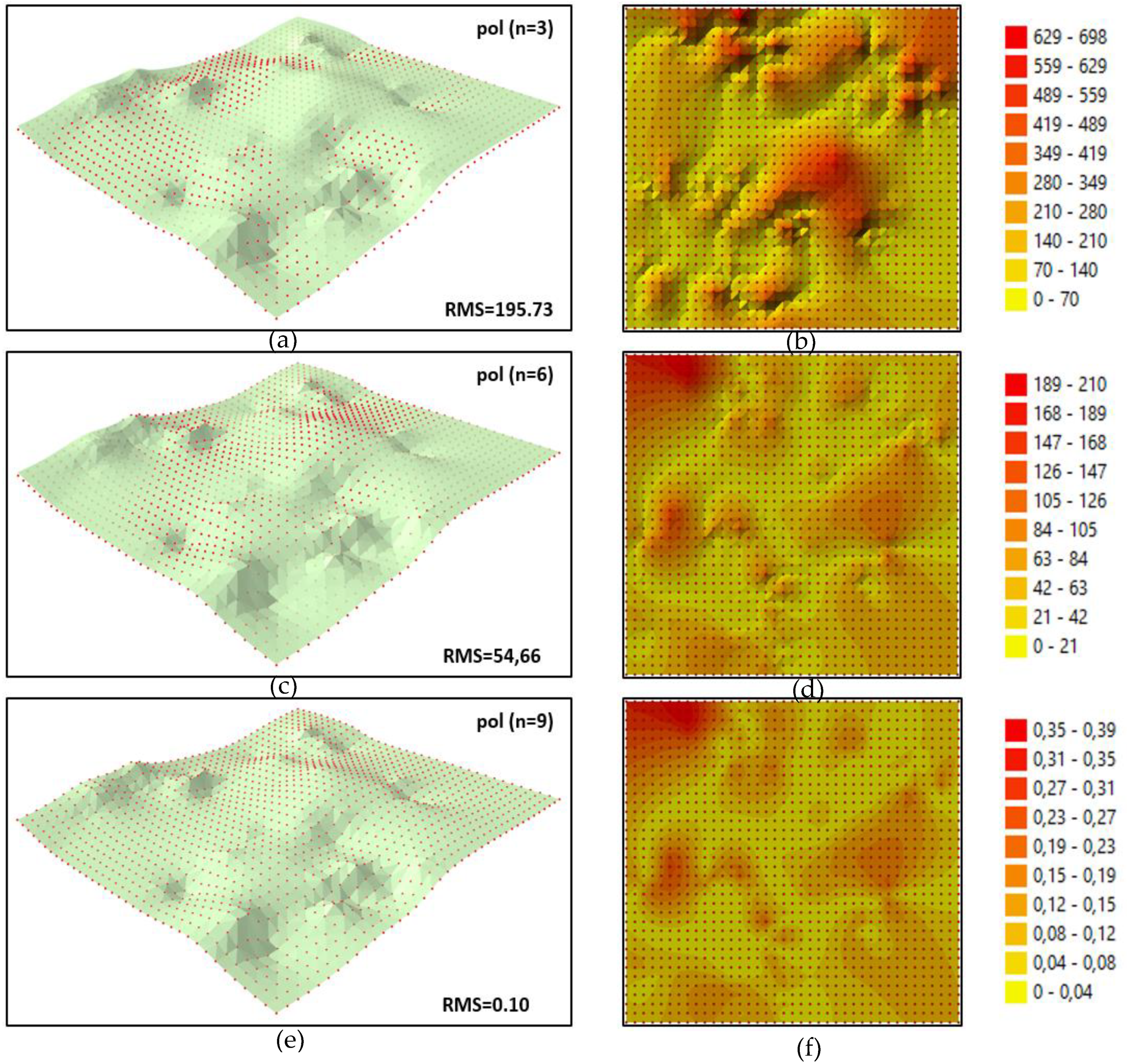
In the presented example, the original surface was created with the use of a GRID structure (t) generated directly from measurement points. The reconstructed surface was generated based on the GRID structure (r) calculated from polynomial coefficients. The differences in node values in both structures were used to determine the RMS. These differences were also used to create differential diagrams presenting the degree of fit between both surfaces. The accuracy with which the reconstructed nodes of the GRID structure were fit to the original surface (2012 data) for different degrees (n) of polynomials generated with the use of all measurement epochs is presented in Figure 5a,c,e.

Differential diagrams generated based on the absolute differences |r_i − p_i| (3) in each node are presented on the right hand side of each diagram. The differences were divided into 10 class intervals. Class intervals differ between diagrams due to considerable differences in the presented values. The RMS coefficient and the presented diagrams support an assessment of the degree of fit between both surfaces and the accuracy with which a given epoch was reconstructed. For nodes that were reconstructed with the coefficient of an approximating polynomial of the 3rd degree (Figure 5a; n = 3), the surfaces were characterised by the worst fit, and the coefficient was the highest (RMS = 195.73). In Figure 5, several reconstructed nodes are positioned above the original surface, whereas other nodes are located under that surface. In the corresponding differential diagram, the digital surface is most deformed at measurement points and in the central part of the model. Most of the presented values are situated within the 0 to 210 interval, which can be attributed to the considerable generalisation of the values reconstructed with the use of the n = 3 polynomial (cf. Figure 4a, b).

The approximating polynomial of the 6th degree (Figure 5; n = 6) better fits reconstructed nodes to the original surface; the RMS is smaller (RMS = 54.66). The differences presented in Figure 5d are three times smaller than in the previous case, and their distribution is similar to interpolation values (Figure 5). Most of the values in Figure 5d are positioned in the 0 to 63 interval, which can be attributed to the smaller generalisation of the values reconstructed in individual nodes of the model (cf. Figure 4d,c). The best fit was achieved for the nodes reconstructed by the interpolating polynomial of the 9th degree (Figure 5e; n = 9), and the differences were within the round-off error. The RMS for the entire object was determined at RMS = 0.10. In the differential diagram for the interpolating polynomial, the distribution of deformations is similar to that observed in the previous case, but most of the presented values are located within the 0 to 0.12 interval. The values determined with the coefficients of the interpolating polynomial can be regarded as error-free (within the range of computational error).

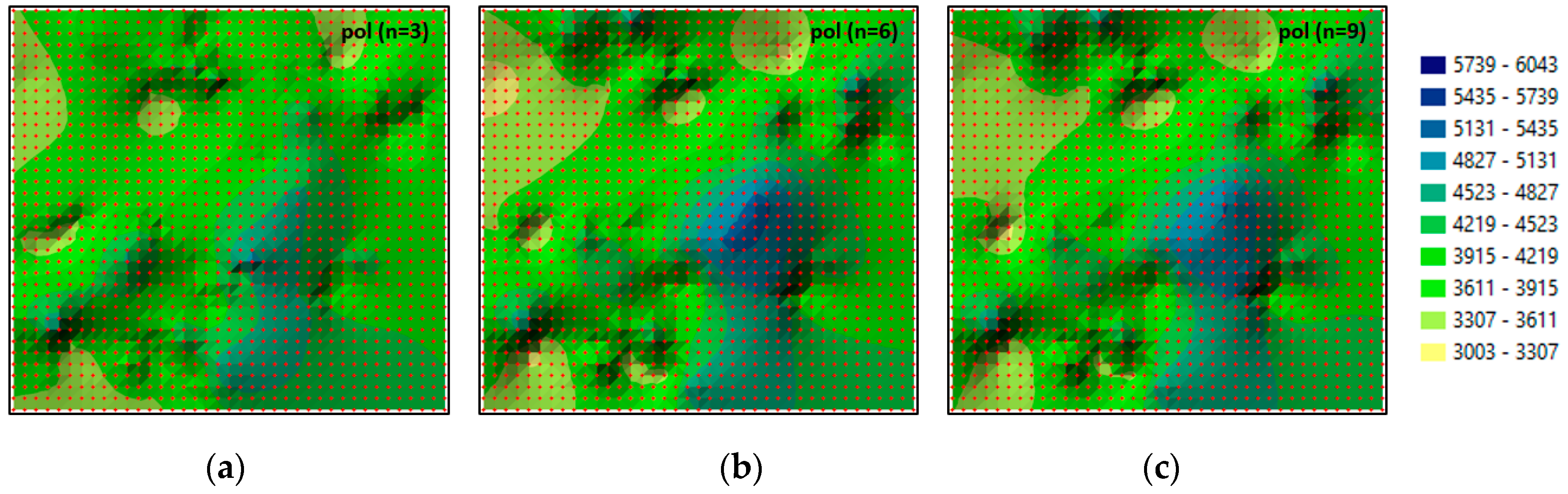
The interpolation surfaces of real estate prices reconstructed for 2012 based on GRID nodes generated for various degrees (n) of polynomials for all measurement epochs are presented in Figure 6. In the presented example (Figure 6), the original surface (Figure 3b) is reconstructed with increasing accuracy based on the nodes generated with the use of polynomials of increasing degree. The original surface (Figure 3b) and the reconstructed surfaces (Figure 6) are presented for identical class intervals. Successive surfaces are increasingly less generalised. The 2012 surface created based on the interpolating polynomial (Figure 6c; n = 9) does not differ from the original 2012 surface (Figure 3b).

An interpolating polynomial also supports the lossless reconstruction of values in all GRID nodes in each epoch. The same surface (reconstructed from a GRID structure) can be generated in a selected epoch (as the original GRID structure) based on measurement data. This approach can be used to reconstruct values in each measurement epoch with the desired accuracy, and the generated values do not have to be saved in separate files. The creation of a single dataset cuts data carrier costs by 25% and speeds up data transfer.

5. Time Series Forecasting for a Selected Measurement Epoch

Individual polynomial coefficients are allocated to each GRID node; therefore, the coefficients saved in a single file can be used to forecast complete GRID structures at any point in time (in any measurement epoch or between epochs). In the predicted structure, each point is determined by solving a system of equations for a curve described by the coefficients of a polynomial (2) and a straight line intersecting the epoch on the time axis (t). In general, the number of generated epochs depends on the time interval adopted for the differences between epochs, which does not have to be identical for individual epochs. If the number of epochs is identical to the number of epochs for determining polynomial coefficients, successive epochs are forecast at the same intervals as the source intervals. A time interval can be freely adjusted, which supports the generation of any number of intermediate epochs or a specific epoch at a given point on the time line (Figure 4 and Figure 7). This missing intermediate structure can be generated based on the nodes created in the neighbouring measurement epochs.

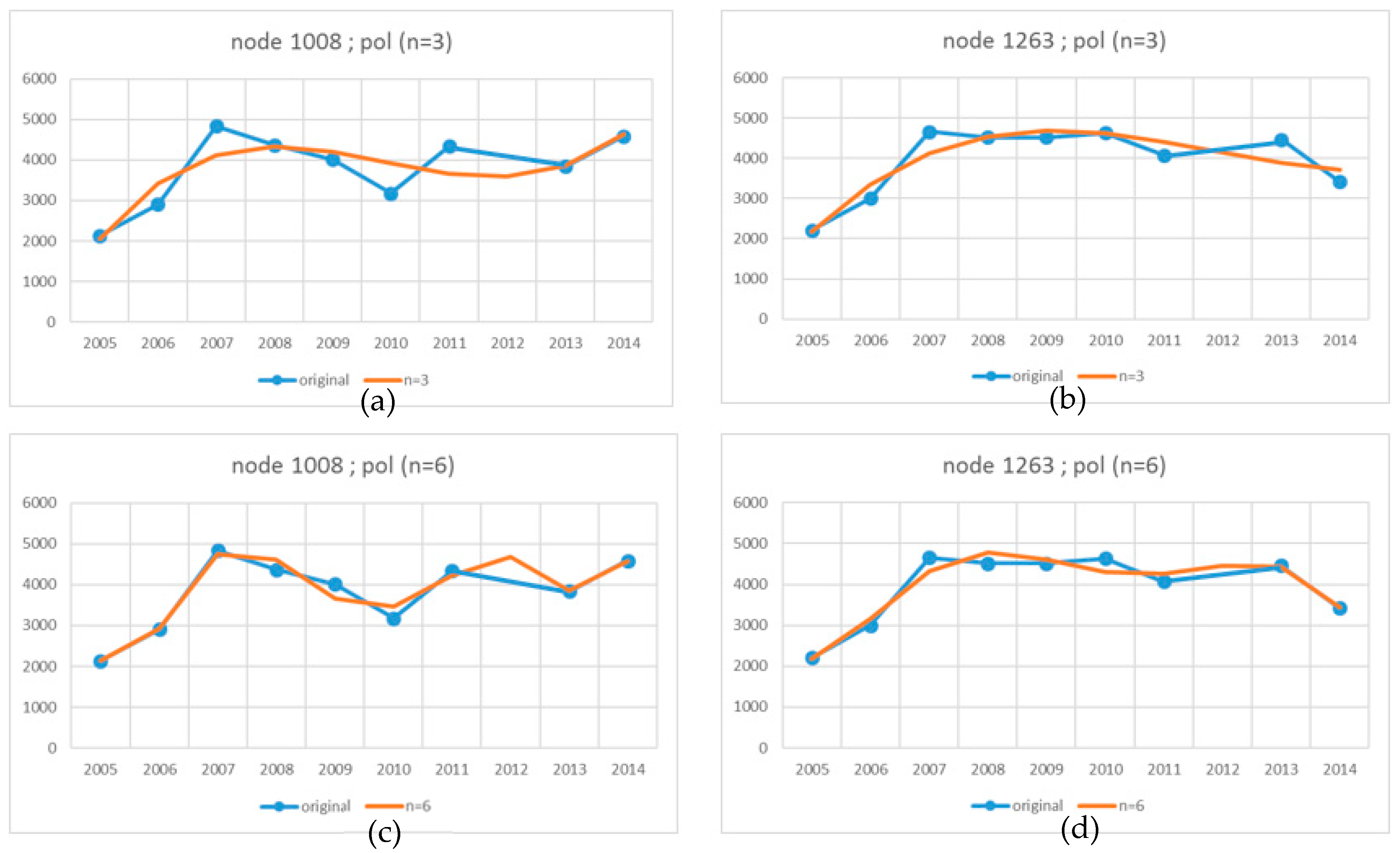
The procedure of forecasting a missing GRID structure is presented on the example of the two nodes that were used in the previous case (Figure 2b and Figure 3b). The missing structure was created with the use of the same measurement data acquired in the 10 epochs, but the 2012 epoch was randomly eliminated. The previously described procedure was used to allocate data from each epoch to all nodes and create a time series (without the 2012 epoch). The selected values were used to calculate the coefficients of polynomials of various degrees (n = 3; n = 6 and n = 8). According to the presented set of equations (1), an interpolating polynomial of the highest degree (n = 8) could be created based on the nine available measurement epochs (E = 9). Individually calculated polynomial coefficients were allocated to each node in a complete GRID structure and saved in a single file. The file containing polynomial coefficients was used to generate all nodes in the measured epochs and in the missing 2012 epoch. The value of (t) was substituted into equation (2) of the polynomial described by the coefficients, and node values were determined in each epoch.

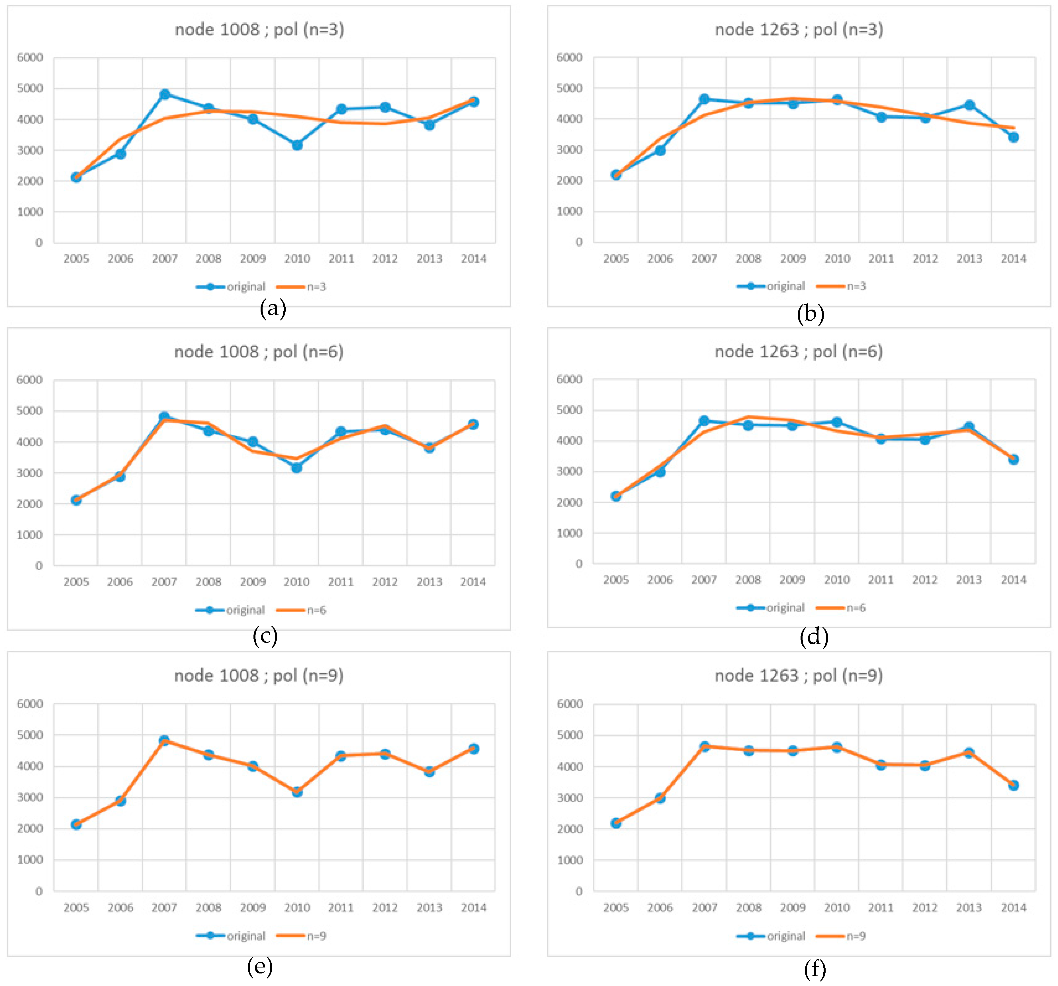
The set of nodes generated for a specific intermediate epoch constitutes an intermediate forecast GRID structure which enables the generation of an intermediate surface at a given point in time. The changes in the original and forecast values in two selected nodes in successive measurement epochs for different degrees (n) of polynomials generated in the absence of the 2012 epoch are compared in Figure 7 (refer to Figure 4 for the legend). 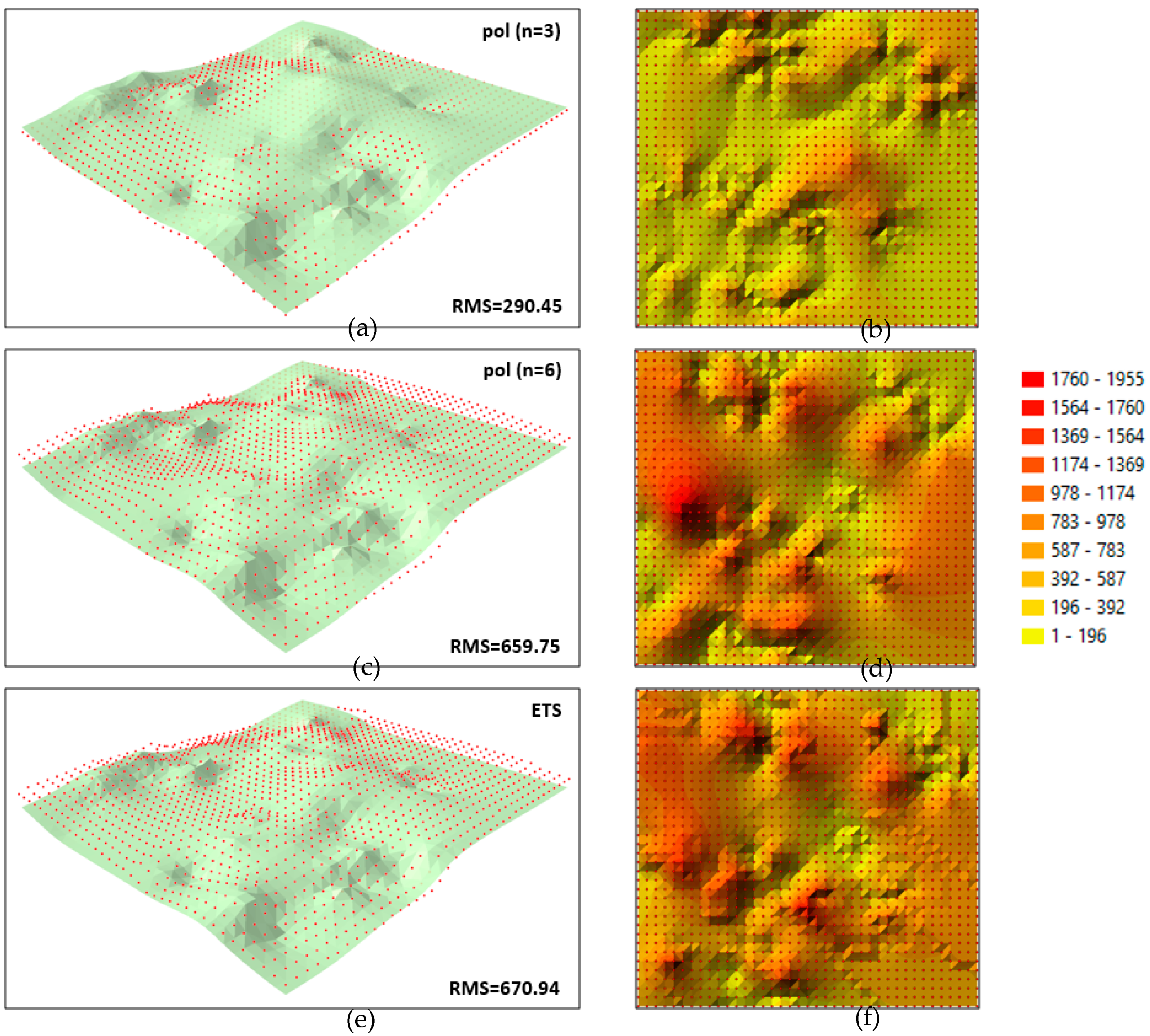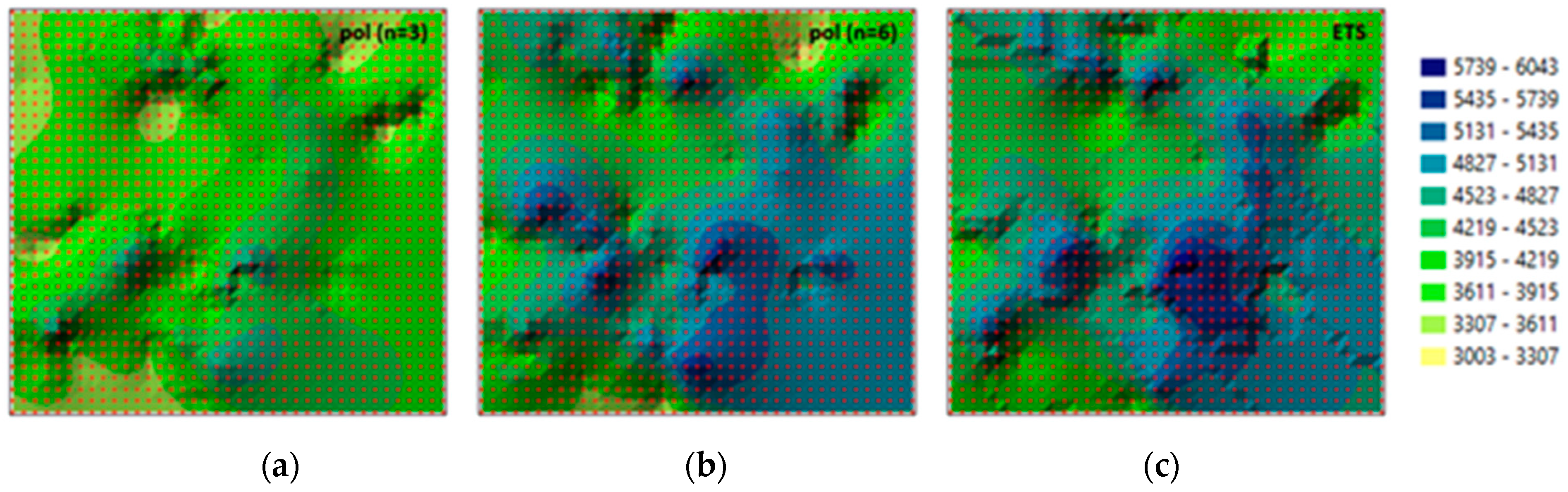Despite the absence of the 2012 epoch, the forecast values are characterised by similar relationships to those in Figure 4 in all cases. Similarly to the previous case, the RMS (3) was calculated and differential diagrams were generated to analyze the accuracy with which the missing 2012 epoch was forecast. The diagrams present the fit between the original surface created based on the measurement points for 2012 and the surface forecast based on the coefficients of polynomials determined in the absence of the 2012 epoch. The accuracy with which the forecast nodes of the GRID structure fit the theoretical surface generated with the use of various methods in the absence of the 2012 epoch is compared in Figure 8. The same interval classification was applied to compare all cases. For the 3rd degree polynomial (Figure 8 a; n = 3), the fit between the forecast surface and the theoretical surface was similar to that presented in Figure 5a. The location of nodes relative to the theoretical surface was similar, and the RMS coefficient was not significantly higher (RMS = 290.45). The differential diagram (Figure 8b) generated for this case was also characterised by a similar pattern of deformations to that presented in Figure 5b. In turn, the 6th degree polynomial produced a less satisfactory fit than when all the measurement epochs were used to determine polynomial coefficients. The majority of the forecast nodes are situated above the original surface (Figure 8c). The RMS for the forecast epoch increased to RMS = 659.75. The differential diagram generated for this case (Figure 8d) is characterised by extreme local deformations which also affect the value of the RMS. Node values were forecast with even lower accuracy when the interpolating polynomial (n = 8) was used. The RMS coefficient was determined at RMS = 2050.63 when this polynomial was applied to forecast the missing 2012 epoch, which makes it unsuitable for use.

The values forecast with the REGLINX.ETS function in MS Excel were also forecast for comparative purposes (REGLINX.ETS calculates or predicts a future value based on historical values by using the AAA version of the Exponential Smoothing (ETS) algorithm.). This function forecasts time series, and it supports the prediction of values based on historical data. The function relies on Exponential Triple Smoothing (ETS) which is an advanced machine learning algorithm. A forecast value is a continuation of historical values on a specified target date which extends the time axis [44,45].

The fit between the nodes generated by ETS and the original surface created for the 2012 epoch based on measurement data is presented in Figure 8e. Similarly to the polynomial (n = 6), the majority of the forecast nodes are situated above the original surface. The value of the RMS is also similar at RMS = 670.94. However, unlike in the previous cases, the differential diagram generated based on ETS results (Figure 8f) is characterized by local stepped surface deformations.

The interpolation surfaces of real estate prices forecast for 2012 based on the GRID nodes generated with the use of various methods (in the absence of the 2012 epoch) are presented in Figure 9. The classification of the forecast real estate prices was identical to that applied to the original surface. The generated surface differs from the original surface (Figure 3b) in all cases (Figure 9). The smallest differences are observed when the 3rd degree polynomial is used (Figure 9a). These differences are similar to the values forecast with the use of the coefficients of the 3rd degree polynomial based on all measurement epochs (Figure 6a).

The surfaces forecast with the use of the 6th degree polynomial (n = 6) and ETS are comparable. In both cases, extreme forecast values have identical locations in the model. Local stepped deformations of the surface model are additionally encountered in the ETS approach. A comparison of the models indicates that the highest forecast values have an identical location to the values in the original model in all cases.

6. Conclusions

The determination of real estate value is of key importance for all operations on the real estate market. Real estate values are the main criterion in investment decisions, and they have an informative role in the economy and real estate management. The appraisal of real estate values requires a thorough knowledge of selling prices and trends in a given time interval; therefore, it is similar to forecasting. In most cases, real estate values are forecast on a local (residential estate, city), regional or national scale, but the results do not contribute information on a given scale. The above can be attributed to the fact that observations at a given “point” are not continuous—real estate transactions are not conducted in a given location at constant time intervals. The proposed methodology can be used to forecast real estate value at a given point in time in a given location, which is of particular importance in real estate market analyses.

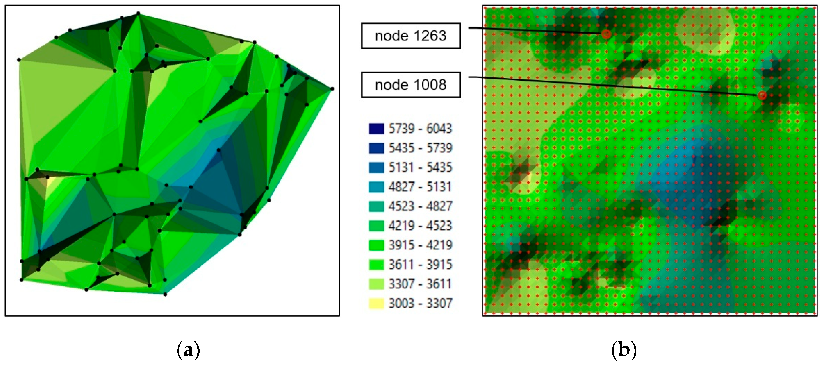
An interpolation algorithm is used during the generation of a GRID structure to determine real estate values at regular network intervals based on irregularly distributed measurement points. One of the greatest weaknesses of GRID structures is that unlike TIN structures, they do not support surface modelling based on the original measurements. However, the desired accuracy can be achieved by selecting the appropriate GRID resolution and the appropriate interpolation parameters. When a TIN structure has a small number of measurement points, the generated digital terrain model (DTM) is characterized by low resolution and low quality. This is not always the case when a GRID structure is applied, because the resolution of nodes in the generated network exceeds the density of measurement points (Figure 3). The above task is not easily accomplished in other structures (TIN, linear models). The resulting model is more accurate in selected locations when surface nodes have higher resolution. An increase in the model’s resolution supports more accurate analyses in selected points, and a complete node network can be used to analyse successive measurement epochs. At the same time, the selected spatial elements can be excluded from interpolation because the resolution of GRID structures is scalable, and therefore, selected nodes can be excluded from analyses.

The solutions presented in this paper can be used to identify data for comparing the prices of real estate registered in various epochs, reconstructing and forecasting price changes over time, and effectively archiving data resources. Data that support the creation of time series for each GRID node can be used to analyze and compare changes in the measured space at selected points of the examined object. The generation of uniform structures in each epoch enables the selection of the values that change over time in each node (located at the same point in each epoch) and the approximation of the observed changes with the use of polynomials of any degree. The information about changes in values in each node is stored in the form of polynomial coefficients, and it can be used to generate the surface of a model allocated to any epoch and to reconstruct and forecast the searched values at any point in time with the required precision. Interpolating polynomials support data reconstruction without loss. A complete GRID structure can be generated in each epoch, and the measured values can be reconstructed and forecast in a given base field with minimum error. Approximating polynomials of a lower degree produce better results in the absence of the forecast measurement epoch. In turn, approximating polynomials of a higher degree generate results that are comparable with the ETS approach, whereas interpolating polynomials are not useful in practice. Polynomial approximation supports the description of changes over time in each node by deploying a series of coefficients that are allocated to each node, which are stored in a single file. The volume of stored data can be reduced by organizing the records from multiple measurement epochs and storing them in a single file. The information stored in databases can be used dynamically with the minimum processing time when the volume of the stored data is minimized. The reduction in the size of the archived datasets speeds up data access and supports real-time analysis. These considerations are particularly important during mass appraisals that rely on extensive sets of data about real estate transactions and prices in analyses covering large areas and long time intervals.