1. Introduction
The study of the sediment yield/supply from the slopes is very important because it has implications for flood hazard—if the volume of sediment exceeds the stream power, the aggradation of the riverbed and the raising of the free surface of the water occur. The process can lead to the overcoming of the river banks/leeves and to the flooding of the alluvial plain [
1,
2]. The correlation between morphological changes in riverbeds, processes of aggradation or degradation and consequent changes in water levels is widely debated and demonstrated, particularly for events with a high return period [
3,
4,
5]. The above mentioned authors suggest that in hydraulic risk modelling to support landscape planning, solid transport and the consequent morphological variations of the riverbed should also be considered. While in lowland areas it is possible that floods are mainly determined by flow discharges—especially for flows with low return period—in mountain environments (small basins with steep slopes) floods are practically always related to strong sedimentary inputs due to landslides and debris flows [
6,
7,
8]. Therefore, a detailed knowledge of sediment production (both in terms of supplying areas and in quantitative terms) is important to correctly define the conditions of hydrogeological hazard and risk in mountain environments.
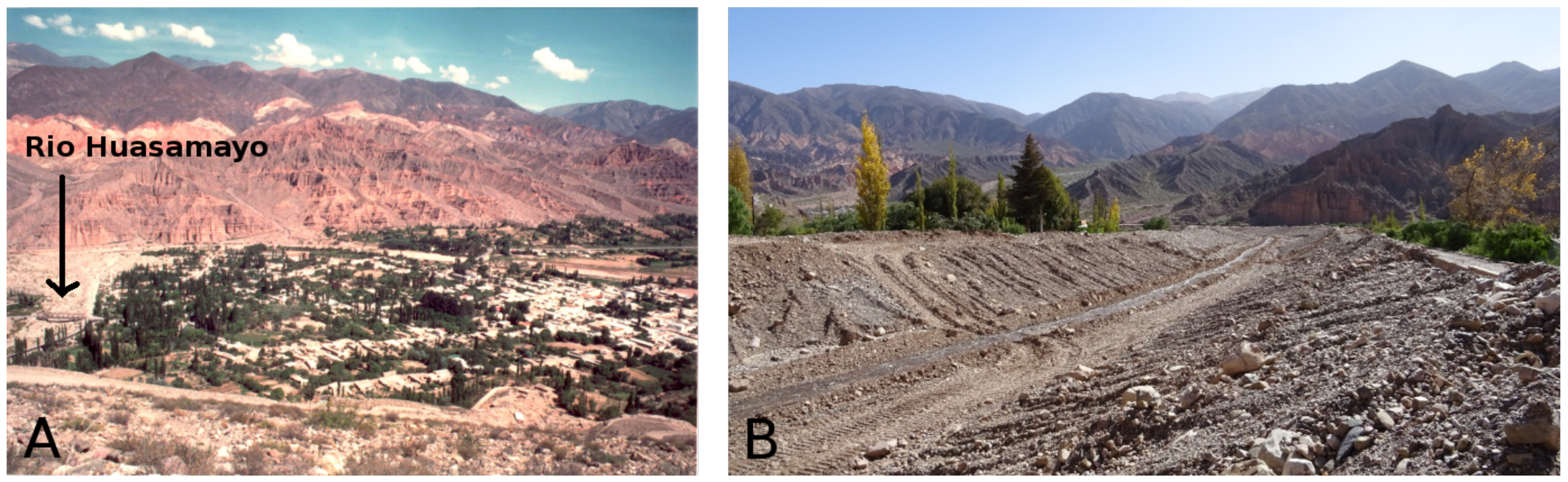
The paper examines a case study—the village of Tilcara, located in the median valley of the Quebrada de Humahuaca (nothwestern Argentina) on the left bank of the Rio Grande, above the large alluvial fan of the Rio Huasamayo, a tributary of the Rio Grande itself (
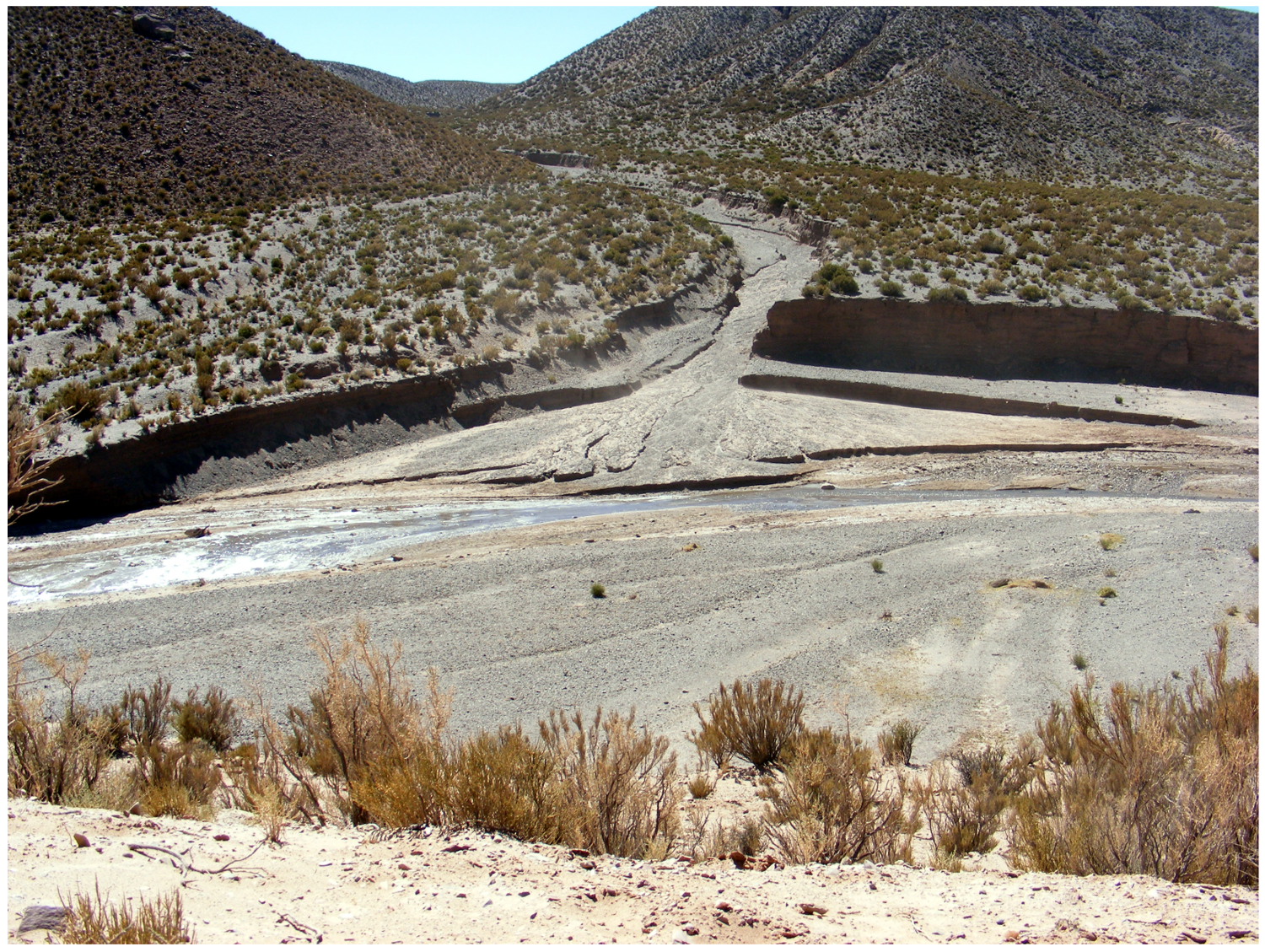
Figure 1A). The final reach of this stream has a superelevated riverbed, forced by artificial banks (
Figure 1B) to flow at higher altitudes than the residential area. This represents a situation of high risk of flooding, as already happened also in the recent past [
9]. Under these conditions, the assessment of the production of sediment within the Rio Huasamayo basin is necessary for the analysis of the causes that have led to the aggradation of the riverbed and therefore to the current conditions of hydrogeological hazard.
To this aim, two methods were used in combination—the Gavrilovic method (Erosion Potential Method (EPM)) and the CORINE method.
Gavrilovic’s model [
10] was originally developed and applied on small basins, with torrential riverbeds; it was later modified, first by Zemljic [
11] and later by Djorovic and Gravilovic [
12]. The last version of the model, applied here, is the one proposed by Gavrilović [
13] in 1988. Several authors have applied the method, especially in non-instrumented basins in the Mediterranean area [
2,
14,
15,
16,
17,
18,
19,
20,
21,
22]. Nevertheless, a comparison with the PSIAC method [
23,
24] showed the same pattern for the predicted sediment yield, with a correlation coefficient of 0.95; it confirms the applicability of the EPM method for semi-arid and arid catchments [
25,
26]. Even the dimensions of the basins studied by these authors are comparable with the analyzed here.
The CORINE method Commission of European Community [
27] allows to identify from a qualitative point of view, the spatial distribution of areas characterized by intense erosion, by obtaining two indexes—PSER (Potential Soli Erosion Risk) and ASER (Actual Soil Erosion Risk—see Methods Section for detail).
The application of the two methods allowed the identification of the main areas of sediment supply and the assessment of the produced sediments. The results were used to define the priorities, types and areas of intervention, at basin level, for the mitigation of the aggradation process in the riverbed.
2. Material (The Study Area): The Quebrada De Humahuaca and the Basin of the Rio Huasamayo
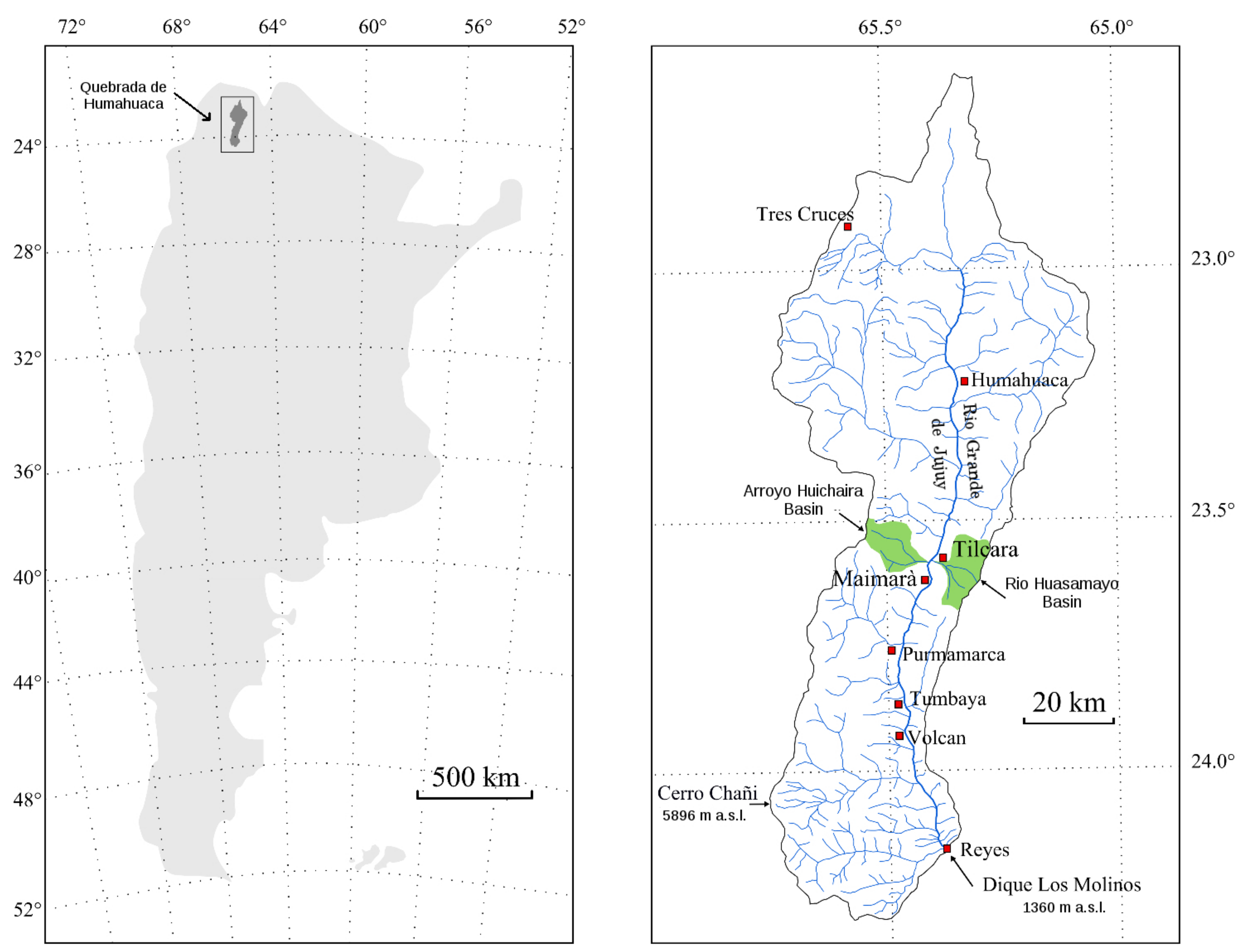
The basin of the Quebrada de Humahuaca, that is, Upper Valley of Rio Grande de Jujuy (Rio San Francisco basin, northwestern Argentina) extends in N–S direction in an area of 6615 km
and is elongated in the same direction of the main geological structures of the Cordillera Oriental of Andes. The difference in altitude is about 4600 m, from Cerro Chani (5896 m a.s.l.), located in the southern part of the basin, until Dique Los Molinos, close to San Salvador de Jujuy, at 1298 m a.s.l. The riverbed, of braided type, is entrenched in a narrow valley extended from the boundary of Bolivia (Tres Cruces) until San Salvador de Jujuy, with an average gradient of 1.4% (see
Figure 2).
The main morphogenetic process affecting the Quebrada de Humahuaca is the physical weathering which, associated with a strong fracturing of the outcropping rocks, produces an intense erosion of the slopes [
28], generating great volumes of unconsolidated material. The concentrated runoff, the gravitational processes and the mass removal (due to frequent and widespread debris flows) cause the over-flooding of the valley floors and the riverbeds aggradation. The consequence of this systematic aggradation is the generation of superelevated riverbeds which, during the rainy season, increase the flooding hazard of the areas close to the streams.
The Quebrada de Humahuaca was elected World Heritage Site by UNESCO in 2003. Therefore, the tourist flow has increased since that date. However, most of the Quebrada is subject to hydrogeological hazard mainly caused by the mobilization of material from the slopes through debris flow processes and by the conspicuous sediments supply from the side tributaries that often cause flooding of the main valley. For example, the Ferrocarril G.ral Belgrano, the only rail link between Argentina and Bolivia, has long since been abandoned due to the frequent flooding that imply high maintenance costs.
2.1. Climatic Characteristics
There are not many meteorological stations in northwestern Argentina and this is a big problem for the hydrogeological monitoring. During the period 1934–1990, in the whole Quebrada de Humahuaca, they were 18; to date, they are less than a dozen and each of them is managed by different Bodies. The data often have no continuity and are difficult to correlate with each other.
Based on the available data, the climate of the Quebrada de Humahuaca appears to be of an arid continental type, with scarce but intense rainfall in the summer season and with very dry winters. Average temperatures are between −5 °C and + 5 °C in winter, reaching a maximum of 25 °C up to 30 °C in summer. Average annual rainfalls fluctuates around 300 mm/yr, concentrated in the austral summer months (December-March). The rainfall gauge that records the minimum rainfalls is Maimarà, located just south of Tilcara (119 mm/yr). To the south this value increases rapidly, so much so that in Termas de Reyes (1800 m a.s.l.), located at the southern portion of the Quebrada de Humahuaca, values of just over 1500 mm/yr are recorded.
Chayle and Aguero [
29] distinguish two zones, inside the Quebrada, clearly different from the climatic and vegetational point of view, located respectively at N and S of Tilcara—(1) the northern one, characterized by a marked absence of vegetation (excluding some xerophilous species, more widespread near Tilcara), with scarce rainfalls and high daily temperature range; (2) the southern one, with higher values of rainfalls, lower daily thermal excursion and with more abundant vegetation, which can reach the characteristics of a humid tropical climate in the sector close to San Salvador de Jujuy.
The average annual temperature in Tilcara is 13 °C, with a maximum of 17.1 °C in January and a minimum of 7.1 °C in July [
30]. However, the daily thermal excursion is very high. Braun Wilke [
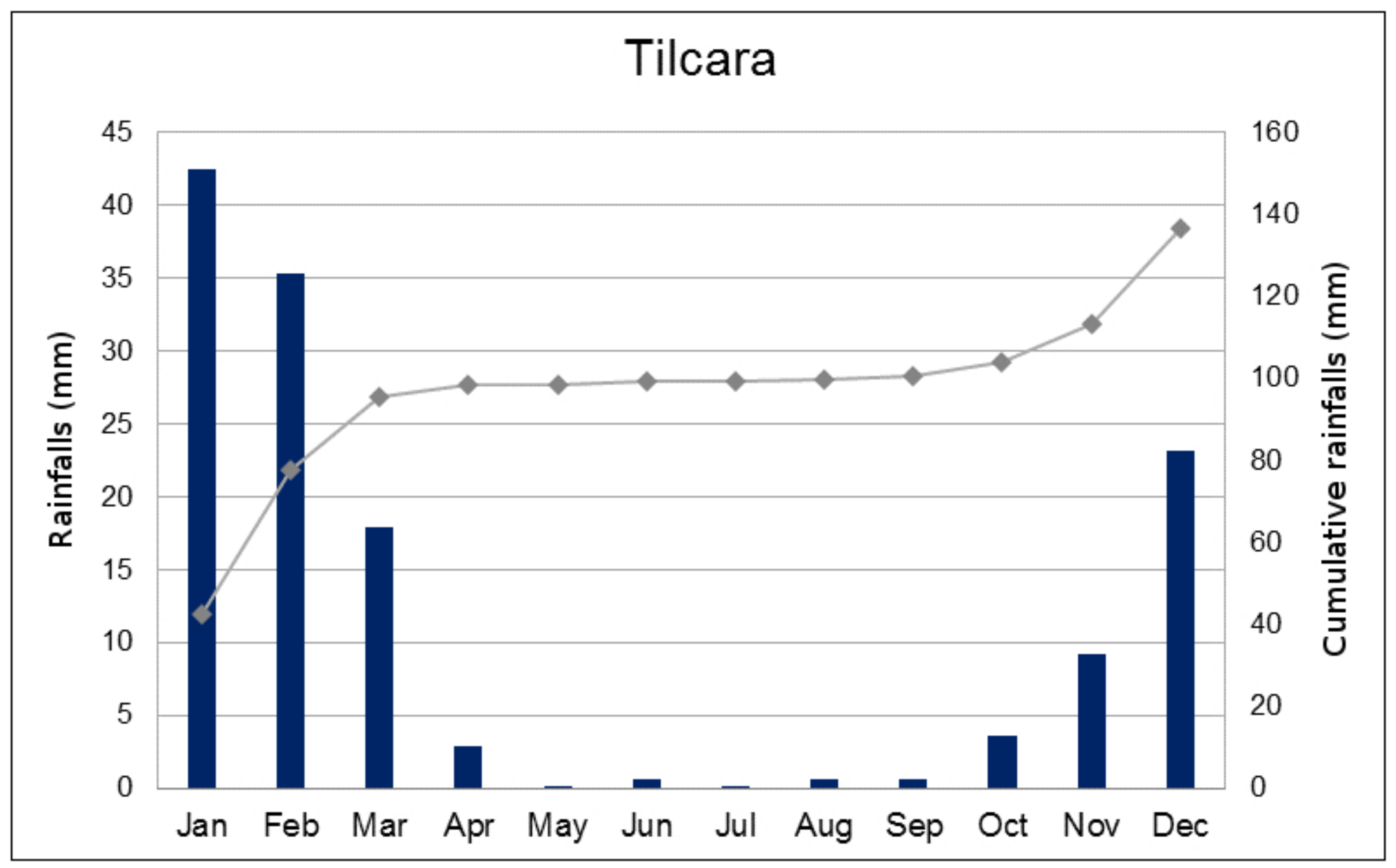
31] determined a temperature gradient for the whole Quebrada which decreases approximately 0.55 °C every 100 m of altitude. The rainfalls regime recorded in the Tilcara gauge (
Figure 3), recorded in the period 1934–1990, shows a dry winter and a rainy summer. The average annual precipitation is 136 mm, as a consequence of the orographic precipitations that are generated with the arrival of the Atlantic anticyclone.
The precipitations regime, with rainfalls concentrated in the summer periods and characterized by intense meteoric events, is the predisposing element to the occurrence of degradation phenomena on the slopes, bare of vegetation, triggering debris flows [
28].
2.2. General Geological Characteristics
In the Quebrada de Humahuaca basin, large outcrops of Precambric and Lower Paleozoic formations prevail, while the formations of the Upper Paleozoic (from Silurian onwards) are practically absent. A stratigraphic gap extends from the Paleozoic to the Lower Cretaceous. However, Tertiary sediments are also present in scarce and fragmented outcrops [
32].
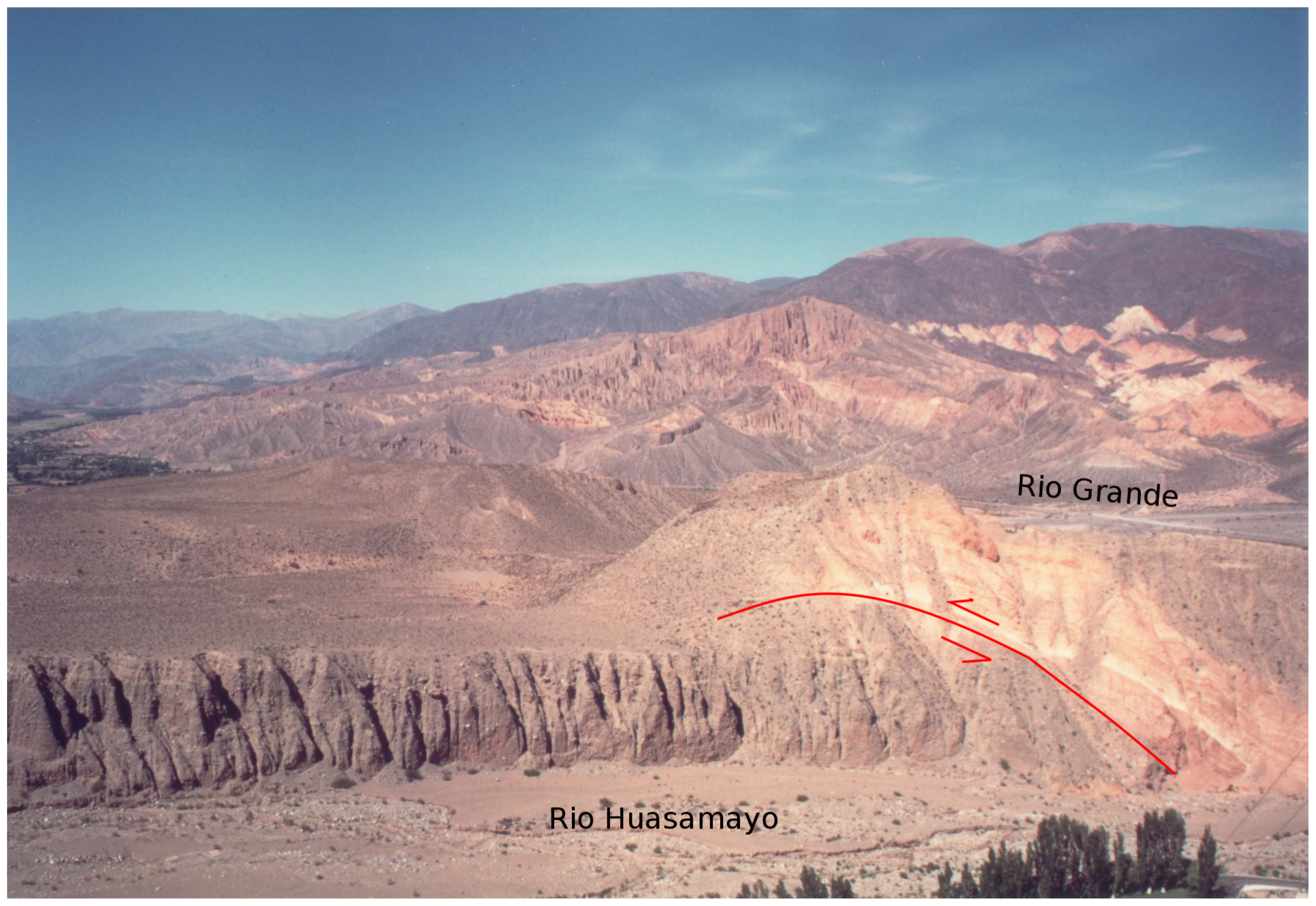
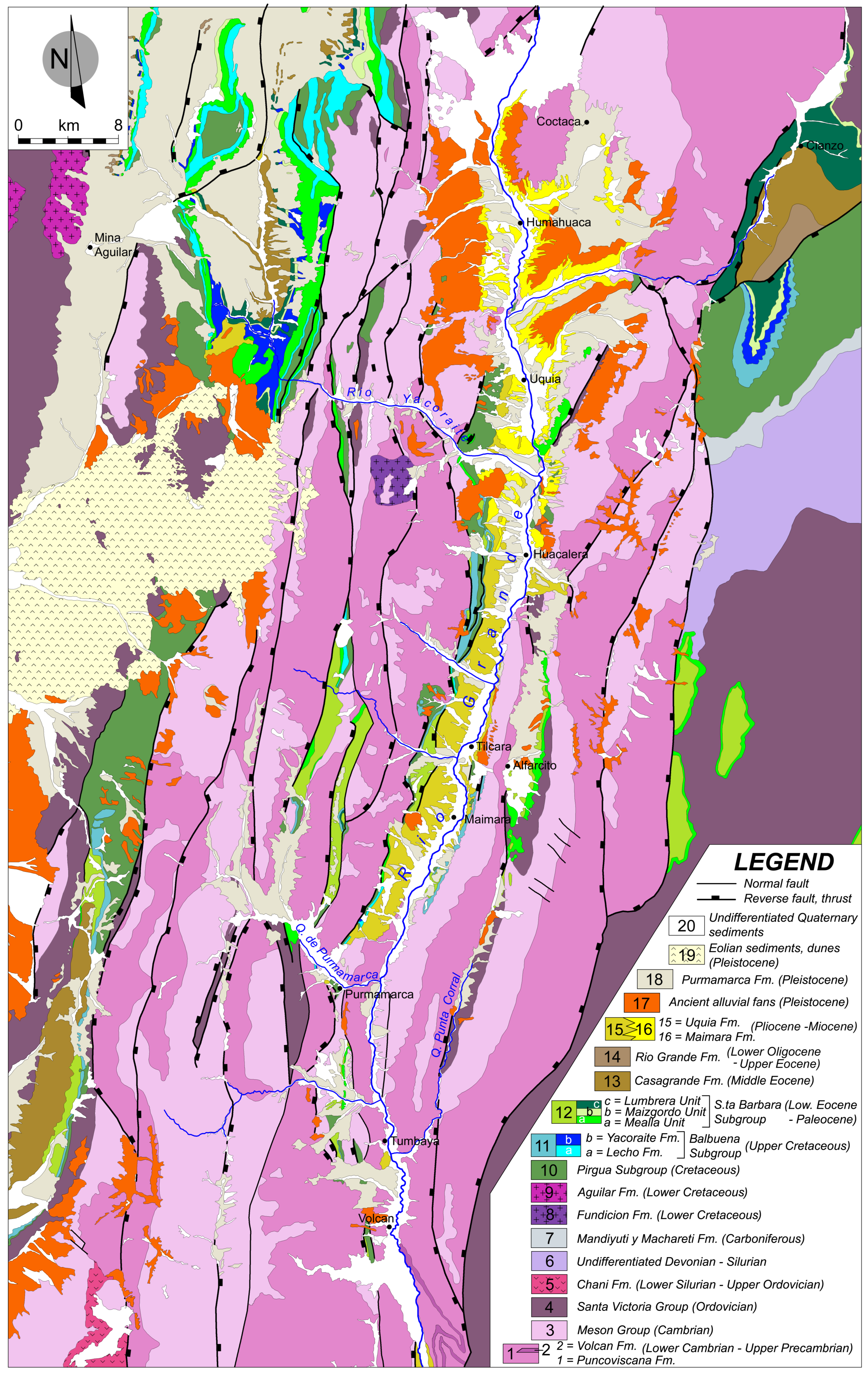
It should be highlighted, instead, the abundant presence of Pliocene and Quaternary clastic sediments that mainly occupy the central area of the valley, just around Tilcara, often affected by tectonic phases (Solis, 1993—
Figure 4). Telescopic fans mark the different uplift phases and the consequent fluvial re-incision of the sediments themselves (
Figure 5).
The most ancient outcropping formation is the
Formación Puncoviscana, of Precambrian age [
33,
34,
35,
36]; it is a very thick formation, about 1500 m, weakly metamorphosed and made up of shales, phyllites, greywackes and quartzites. Conglomerates and sandstones of continental environment, in river facies, belonging to the Units of the
Grupo Mesón of the Cambrian [
33] and conglomerates, sandstones and clays in continental shelf facies, belonging to the Units of the
Grupo Santa Victoria of the Ordovician [
33,
37,
38,
39] overlap with angular unconformity.
There are few outcrops of formations referable to the Upper Paleozoic; the outcrops of the Mesozoic formations should instead be highlighted. The oldest are magmatic rocks from the Lower—among these, particular mention should be made of the
Formación Aguilar, a granitic pluton, very important from an economic point of view for its Pb and Zn mineralizations [
40,
41,
42,
43,
44,
45], still object of mining cultivation (Mina Aguilar, at W of Humahuaca).
The Mesozoic-Tertiary sedimentary cycle (Cretaceous-Paleogene) is represented by
Grupo Salta [
46,
47], subdivided into the subgroups
Pirgua, Balbuena and
S.ta Barbara [
48,
49,
50]. The formations of the
Grupo Salta are almost entirely in continental facies and constitute the deposits of an intracratonic rifting phase [
51] to which the placement of the already named Aguilar granites is connected in the study area. The overlapping formations,
Formación Casagrande (Middle Eocene) [
52,
53,
54] and
Formación Río Grande (Miocene) [
55], show the same depositional environment and consist of conglomerates and sandstones in fluvial facies (braided type), with clayey levels, which are rarer upwards. The following formations are also found in continental facies—the
Formación Maimará [
56] which covers the central sector of the Quebrada, consisting of sandstones and conglomerates with clayey matrix; referable to ancient syntectonic alluvial fans raised with respect to the current thalweg of the Rio Grande; and in heteropia of facies towards the north-west, the
Formación Uquía [
57], consisting of yellow sands with intercalated conglomerates in more frankly fluvial facies (braided). The sediments of the ancient alluvial fans of Quaternary age are the product of the recent morphological evolution of the Quebrada and they are in great quantity inside the depression of Humahuaca. They consist of gravels that also incorporate large boulders with a stratified structure and levels of volcanic scoriae.
The
Formación Purmamarca of the Pleistocene age [
32,
58], on the other hand, has more morphological than chronostratigraphic significance; although it is made of the same material of alluvial formations as already described, it represents a morphological reference level of local importance and it is especially present in the Quebrada de Purmamarca, from which it takes its name. The gravels and the embedded boulders of phyllites and tillites come mainly from the
Formación Puncoviscana which outcrops in the neighboring areas. Its structures and the poor sorting make it possible to refer to deposits produced by debris flows processes and, secondarily, by fluvial processes, connected to the Pleistocene periglacial climatic conditions. The dune fields refer instead to accumulations of aeolian processes affecting the Puna, west of the Quebrada. These are aeolian sands that constitute alignments of longitudinal dunes and barchans. Finally, all the more recent deposits, from the Pleistocene to the Holocene, of predominantly fluvial origin (gravels, sands, the last generation of alluvial fans, more recent terraced sediments of the Quebrada) are identified with the term “Undifferentiated Quaternary”.
Figure 6 (from Cencetti [
28]) shows a medium-scale geological map of the central portion of the Quebrada de Humahuaca, more specifically the subject of this note.
2.3. The Rio Huasamayo
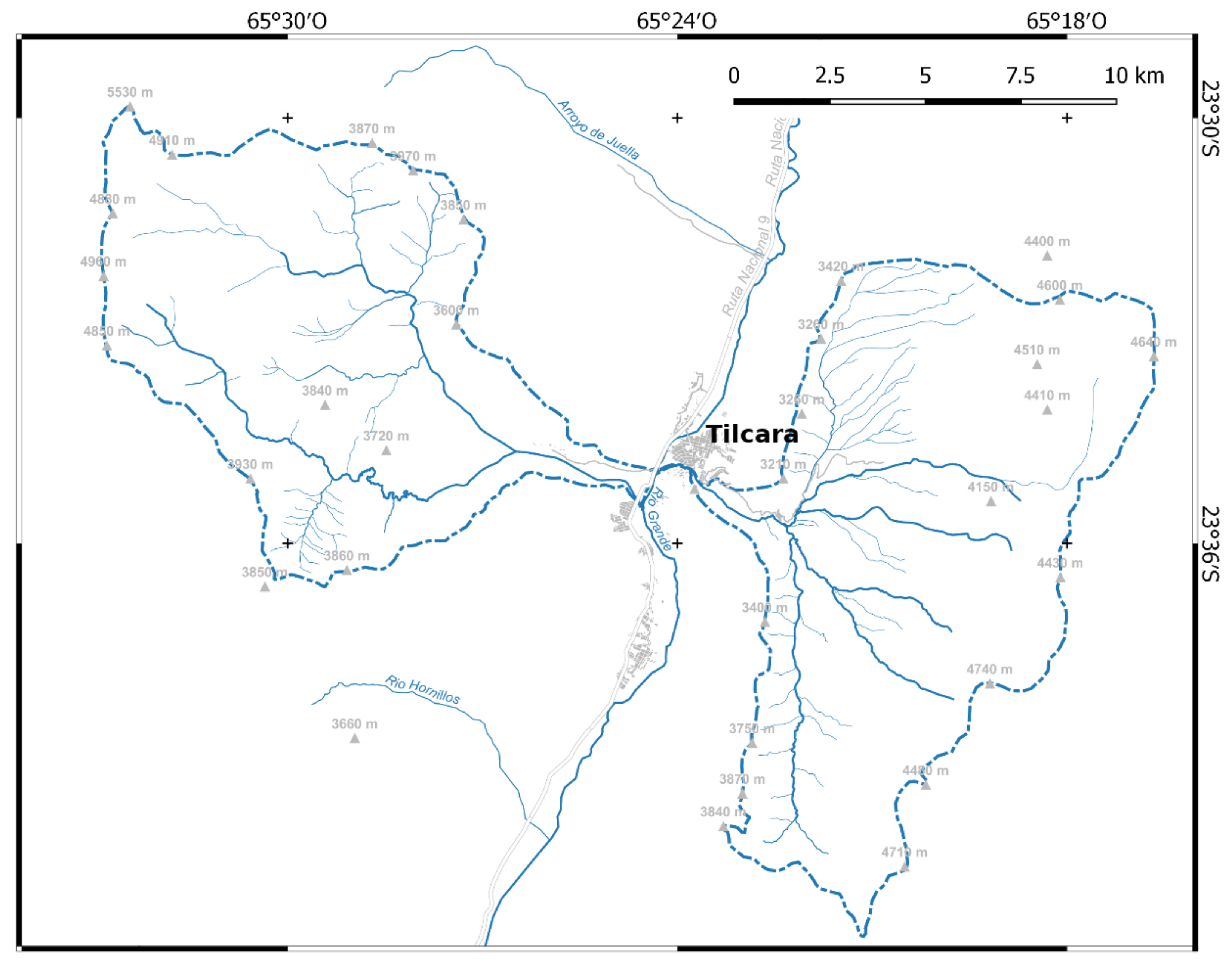
The village of Tilcara is located close to the confluence between the Rio Grande and two tributaries (
Figure 7), respectively the Rio Huichaira on the right bank, and the Rio Huasamayo on the hydrographic left. The Rio Huasamayo, subject of this note, originates from the confluence of five streams and reaches the Rio Grande (Quebrada de Humahuaca) at 2450 m a.s.l., with a length of just 4 km and with a very high average gradient (12%). Its watershed has an area of about 114 km
; its tributaries originate between Ovejería and Suncho Grande mountains, at altitudes between 4600 and 4850 m a.s.l., and flow along slopes characterized by high steepness, into a gorge (
Garganta del Diablo).
The Rio Huasamayo, starting from about 95,000 years, built an alluvial fan extending for about 5 km
[
59] where the town of Tilcara is located. It is a mixed-type alluvial fan, formed both by the systematic aggradation of material brought by the stream and by gravitational processes such as debris flows [
9,
59].
Actually, the Rio Huasamayo is forced to flow into a narrow fan sector within an artificial bed. This condition and the continuous aggradation have led to an increase in altitude of its thalweg, which is located at a higher altitude than the inhabited area of the village of Tilcara. This situation represents a clear risk of flooding for the town. Rivelli and Zelarayan [
9] have carried out a census, based on historical data, of the floods caused by the Rio Huasamayo, identifying over twenty catastrophic events from 1867 (the first documented) to 2016. The same authors have carried out a hazard analysis, through a zoning of the Tilcara alluvial fan, identifying the areas that have been most affected in the past (and therefore may be in the future) by the Rio Huasamayo floods.
To solve the problem, Marcato et al. [
60] proposed the deviation of the Rio Huasamayo before the village, building an artificial channel working as drainage channel. The preservation of Tilcara, however, would not reduce the hydraulic risk, which would only be transferred downstream the Quebrada towards the village of Maimará. Then, we propose an alternative solution, intervening at the origin of the problem. By way of direct observations and the study of existing maps and satellite images, by applying the method proposed by Gavrilovic and using the CORINE Project data, it is possible to estimate the volume of material produced by the Rio Huasamayo watershed, identifying the main supplying areas where focused interventions for the control of solid transport could be realized [
9].
3. Methods
In the literature there are several formulations and quantitative models that allow assessment of soil erosion, that is, USLE—
Universal Soil Loss Equation (i.e., References [
61,
62,
63]; RUSLE—
Revised USLE [
64,
65,
66]; USPED—
Unit Stream Power—based Erosion Deposition [
67]. They differ in the input data and in the processing and accuracy of the results. Nevertheless, they are not usable due to the lack of necessary input data such as specific data about rainfalls.
So, in order to estimate soil erosion in the Rio Huasamayo catchment area, the following methods have been used:
CORINE (COoRdination of INformation on the Environment) method [
27], of qualitative type, useful for identifying the distribution of areas characterized by intense erosion;
EPM (Erosion Potential Method) proposed by Gavrilovic [
10], of quantitative type, capable of evaluating the average production of sediments in a watershed. This model is based on empirical formulas that allow us to obtain the volume value of sediment production. It takes into consideration some geomorphological, climatic, lithological and vegetation parameters and allows a theoretical estimate of the volume of material produced by erosion in a river basin. The model uses a reduction coefficient, to consider that not all the produced material reaches the closing section of the hydrographic basin due to redeposition processes. Then the amount of debris carried by the stream through closing section is determined.
3.1. Application of the CORINE Method
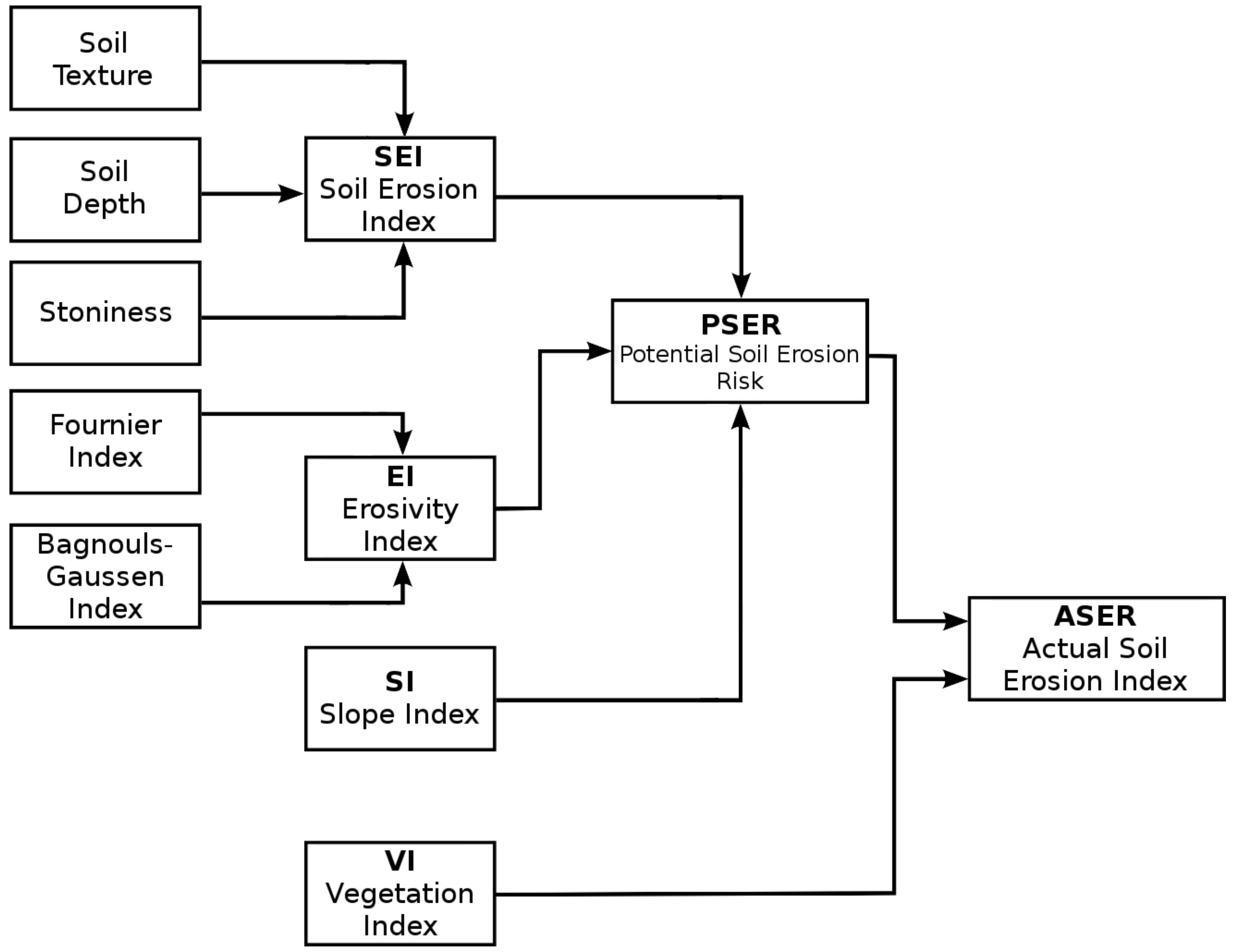
The CORINE method allows to obtain two indexes:
PSER (Potential Soil Erosion Risk) which indicates the susceptibility of soils to erosion, considering the factors linked to land use, climatic and topographic conditions;
ASER (Actual Soil Erosion Risk) which indicates erosion under current conditions of land use and vegetation cover.
The estimation of erosion according to this method develops through two main phases (
Figure 8).
In a first step the PSER index is calculated, by adding the Soil Erosion Index (SEI), the Erosivity Index (EI, due to climate conditions), and the topographyc Slope Index (SI, due to the incline of the slope), by determining values that correspond to different classes. With this operation we obtain a value of soil susceptibility to erosion, just called Potential Soil Erosion Risk (PSER).
In particular, the
Soil Erosion Index (SEI) is evaluated considering the
texture of soil, its
depth (i.e., its thickness, interpreted as the distance between the surface and the upper part of the bedrock or of the original unaltered material, divided into 3 classes: >750 mm; 250–750 mm; <250 mm), and the superficial
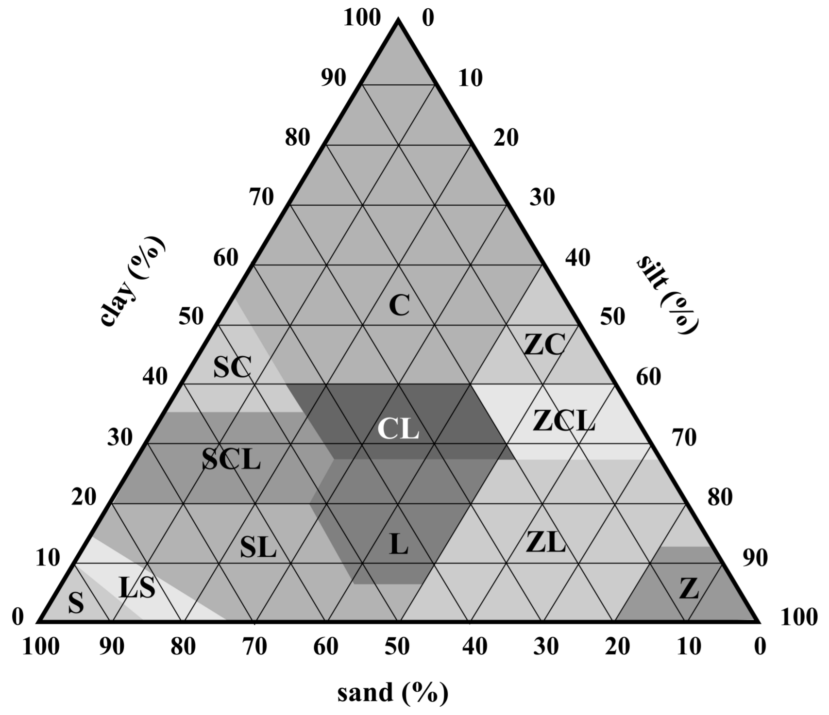
stoniness, that is, the greater or lesser presence of unconsolidated material of coarse grain size (>20 mm of average diameter), divided into 2 classes—completely protected soil (percentage of coverage% >10); not protected soil (percentage of coverage% <10). The grain-size characteristics of the soil allow to define three granulometric classes (
Figure 9;
Table 1) obtained on values proposed by the United States Department of Agriculture (USDA [
68]).
The value of
Soil Erosion Index (SEI) is obtained from the product:
and based on the result, the index value is assigned as shown in
Table 2.
The
Erosivity Index (EI) is obtained starting from the Fournier-Arnoldus index (FI: Fournier Index, Arnoldus, [
69]) and from the aridity index of Bagnouls-Gaussen (BGI, Gaussen, [
70,
71]). The Fournier index, modified by Arnoldus, is obtained from the expression:
where:
The value of FI is assigned as in
Table 3.
Bagnouls-Gaussen’s aridity index (BGI) is calculated on the basis of the monthly moisture balance, estimating the evapotranspiration starting from the temperature. It is obtained by applying the equation:
where:
i = month ith;
= average monthly temperature (°C);
= average monthly rainfalls (mm);
= proportion of month , where (obtained by linear interpolation).
To estimate the value of BGI, it is necessary to calculate by linear interpolation the dates in which the period begins or ends where
. For this reason, it is assumed that the temperature and precipitation values are produced on the fifteenth day of the month. The value of BGI is then assigned as in
Table 4.
The value of the climatic
Erosivity Index (EI) is then obtained from the product:
assigning to EI class the value as in
Table 5.
The
Slope Index (SI) is established starting from topographical characteristics, dividing the territory into square cells (1 km
), in which the average value of the slope is calculated. The SI is assigned to this slope according to the range of values as in
Table 6.
The
Potential Soil Erosion Risk (PSER) is then obtained by the product:
and its value is attributed as in
Table 7.
In the second step, the
Actual Soil Erosion Risk (ASER) is obtained by integrating the PSER with the
Vegetation cover Index of the soil (VI). In particular, the VI is obtained by dividing the land according to the type of vegetation, as in
Table 8.
The ASER is obtained starting from the PSER and from the VI, using the matrix shown in
Table 9.
The result of the application of the CORINE model allows us to define the areas with high risk of erosion (class 3), where control practices are necessary, areas of medium and low risk (class 2 and 1), where agricultural practices do not require specific conservation techniques, and finally, areas with zero risk (class 0).
3.2. Application of the EPM (Gavrilovic)
The evaluation of material leaving the basin (
G) is based on the following relation:
where
W is the volume of solid material produced annually by erosion (m
yr
), obtained by the Equation (
7), and
R is the reduction factor (Equation (
10)):
where:
T = temperature coefficient, defined by Equation (
8).
h = average annual rainfalls (mm);
z = coefficient of relative erosion, defined by Equation (
9);
n = experimental coefficient (generally = 3);
F = area of the basin (km).
where
is the average annual temperature in the basin (C).
with:
X = soil coefficient, depending on the vegetational cover;
Y = soil erosivity coefficient, as a function of the prevalent outcropping lithotypes;
= coefficient that expresses the degree and type of erosive processes;
I = mean slope of the basin, expressed in percentage.
In
Table 10,
Table 11 and
Table 12 are reported the values of X, Y and
to be assigned to the various areas (sub-basins), having homogeneous lithological, vegetational and geomorphological characteristics, in which the main river basin is subdivided (Gavrilovic, [
13]).
To define the coefficient
z the weighted averages of the values are used of each coefficient relative to the corresponding areas. The reduction factor
R, according to Zemljic [
11], is given by the following expression:
where:
O = basin perimeter (km);
D = mean elevation, determined by the hypsometric curve (km);
L = lenght of the main stream in the basin (km);
= cumulative lenght of the tributaries (km);
F = basin area (km).
4. Data and Results
Applying the method proposed by Gavrilovic [
13] and using the data from the CORINE Project [
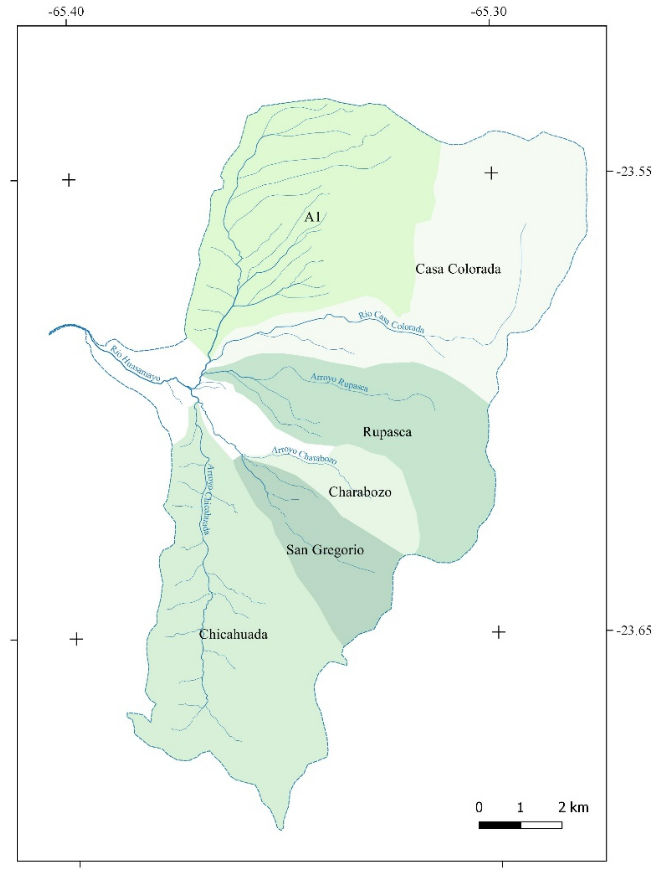
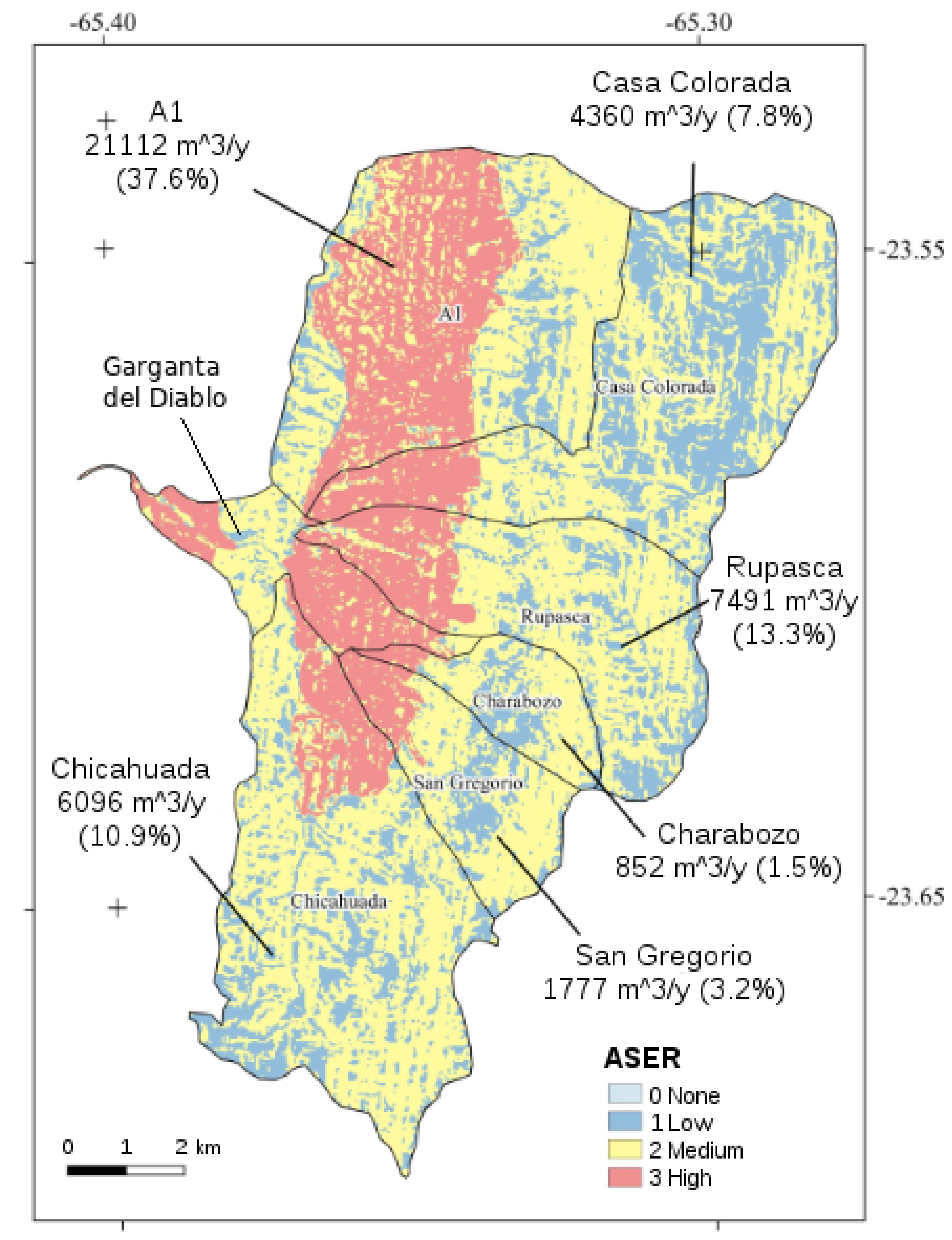
27], the volume of material produced by the Rio Huasamayo basin was estimated and the main areas that constitute the source of this material were identified, that is, characterized by greater erosion. In order to better analyze the dynamics of the Rio Huasamayo, its basin has been divided into six sub-basins (
Figure 10) renamed as follows—A1, Casa Colorada, Rupasca, Charabozo, San Gregorio and Chicahuada (their main physiographic parameters are reported in
Table 13).
The method was applied by generating, in a GIS environment, a layer for each index proposed by the CORINE method [
27]. The Soil Erosion Index (SEI) was determined taking into consideration the geological map
“Ciudad de Libertador General San Martin, 2366-IV”, in scale 1:250,000 and the respective explanatory notes [
72], as well as the observations made in the field and from aerial photos by the authors. The classification proposed by the method has been adapted according to the outcropping lithotypes (
Table 14).
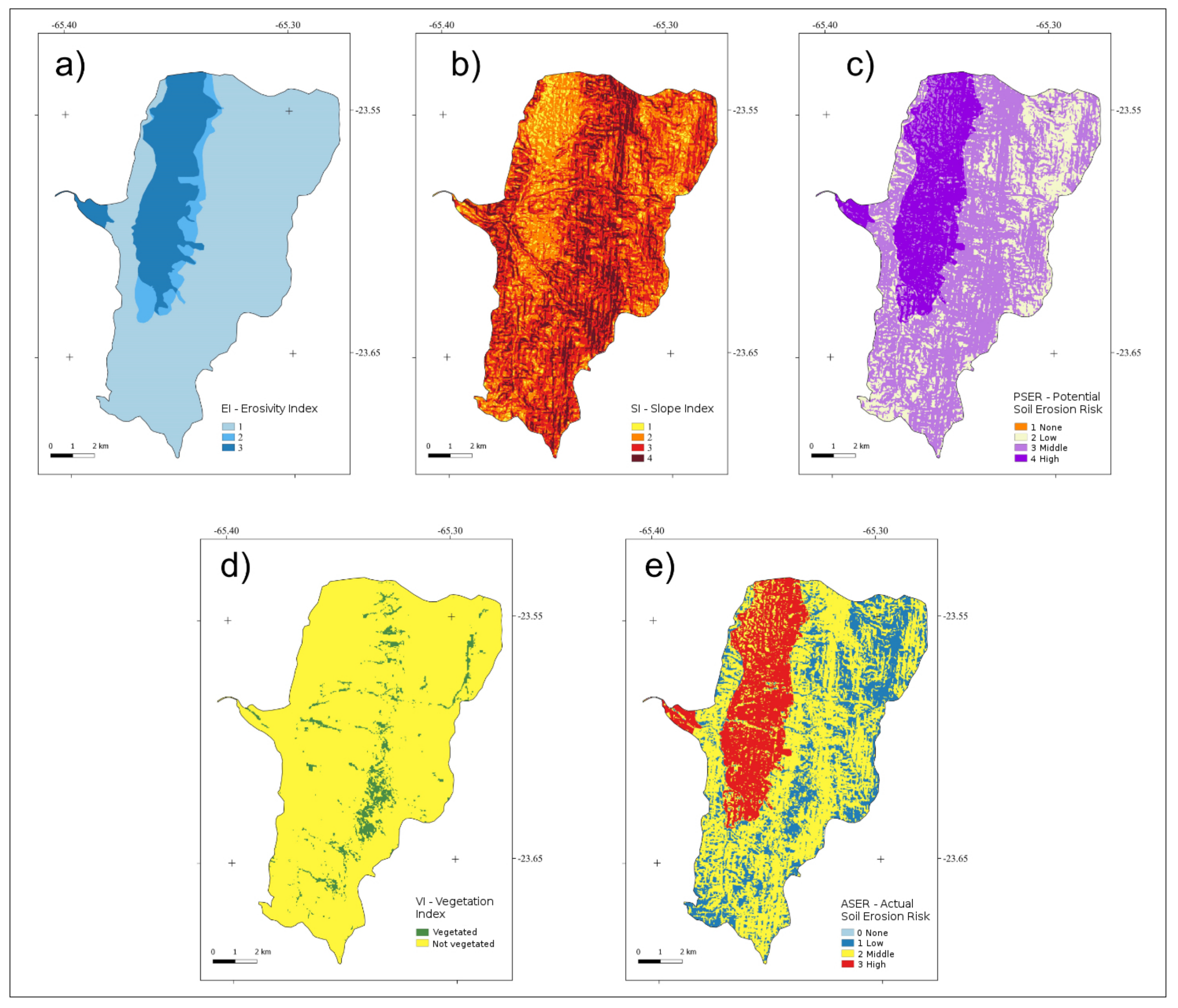
Due to the lack of meteorological data available and above all the temporal continuity of the measurements, for the determination of the climate erosion index EI (Erosivity Index) the records of rainfalls and temperature acquired by the Tilcara rain gauge were used in its last year of activity, 1990. The Fournier-Arnoldus index (FI) and the Bagnouls-Gaussen index (BGI) were applied homogeneously for each sub-basin—respectively, a value of 46 was obtained, which corresponds to class 1 (very low) and a value greater than 180 (maximum value for classification), thus assuming a class 4 (very arid). The value of the Erosivity Index (EI), obtained from the product of these two, falls therefore in the middle class (2). The Slope Index (SI) was determined using a special function in GIS environment that allows to calculate and classify in pixels the slopes, starting from the ASTER GDEM (30 m resolution).
The ASTER GDEM Validation Team [
73] estimated a vertical accuracy of 6.1 m in flat and open areas and 15.1 m in mountainous areas, largely covered by forest.
The presence of vegetation in the basin was determined through the use of Landsat satellite images that allowed, again in the GIS context, the calculation of the NDVI index [
74]. This index is determined by the ratio between the reflectance values NIR (Near InfraRed) and R (Red), according to the relation:
The terms refer to the spectral absorption of chlorophyll in the Red (R, band 3 of the Landsat) and in the near Infrared, where the same reflectance is strongly influenced by the leaf structure (NIR, band 4). By means of this index, it was possible to identify the vegetated areas and then to define a layer for the Vegetation Index with non-vegetated areas and vegetated areas (
Figure 11).
The method proposed by Gavrilovic [
13] has allowed estimation of the average production of sediments in the Rio Huasamayo basin and its sub-basins. As a first step, the values of the parameters used by this method (coefficients X, Y and
) have been attributed, based on
Table 10,
Table 11 and
Table 13.
For other parameters, derived by meteorological data, temperature and rainfall gradients with respect to elevation have been considered. This choice allowed us to assign appropriate values for each basin.
4.1. Pluviometric Gradient
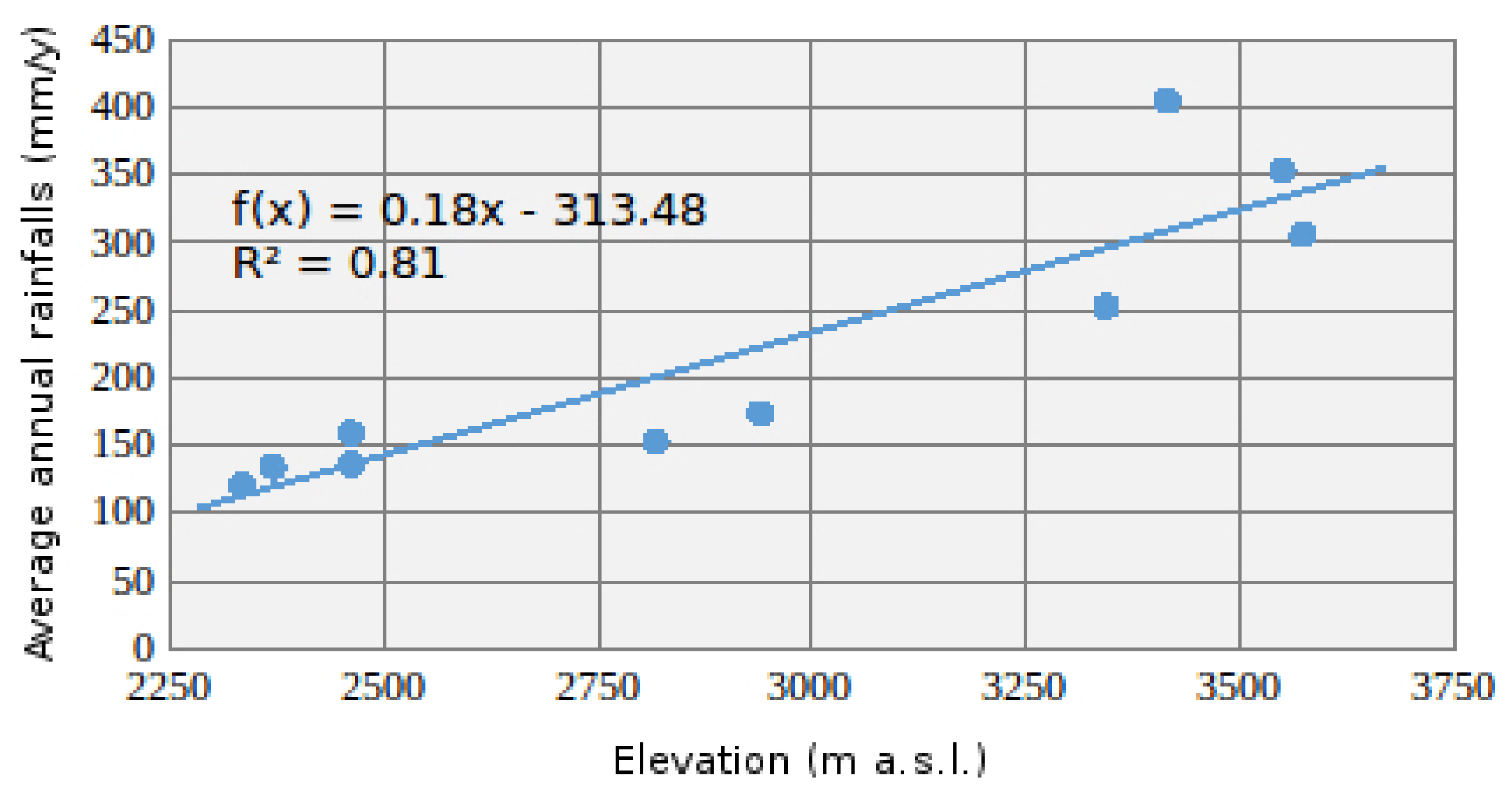
For the rainfalls, a regression line has been defined, examining the gauges of Maimará, Vivero Hornillos, Tilcara, Huacalera, Uquia, Humahuaca, Iturbe, Cianzo, Placa de Aparzo and Coctaca. These record a linear trend (
) with a positive precipitation gradient which increases by about 18 mm every 100 m (
Figure 12), according to the following equation:
4.2. Temperature Gradient
Regarding the temperature values, the gradient proposed by Braun Wilke [
31] was used. The temperature decreases of about 0.55 °C every 100 m, according to the following equation:
5. Results Obtained From the Application of the Method
The results obtained are shown in
Table 15. The Gavrilovic method estimates an annual production of 56,179 m
yr
for the Rio Huasamayo basin, of which 74.2% comes from the analyzed sub-basins. In particular, the percentage incidence for each sub-basin is—Chicahuada 10.9%, A1 37.6%, Casa Colorada 7.8%, Rupasca 13.3%, San Gregorio 3.2%, and the Charabozo 1.5%.
The combined application of the two methods made it possible to identify the sub-basins that provide a greater sediment supply. The areas with a high ASER Index (class 3—
Figure 13) are distributed downstream of the Garganta del Diablo, an area in which the Rio Huasamayo basin narrows towards the confluence with the Rio Grande de Jujuy and, above all, in the area with the NS direction between the Sierra de Tilcara (4600 m a.s.l.) and the Cordon de Alfarcito (3200 m a.s.l.).
These two areas have in common the outcrop of Quaternary clastic rocks, consisting of conglomerates with coarse sandy matrix. The lithological characteristics of these sectors played a fundamental role in determining the high ASER index obtained. This observation is reflected in the Gavrilovic method. In fact, the sub-basin A1, which has most of its area in class 3, potentially generates about 37.6% (21,112 m yr) of the total sediments exported by the entire Rio Huasamayo basin. The sub-basin A1 has also the maximum value of G (specific G = volume of solid material produced annually by erosion per km).
6. Discussion
6.1. Causes of the Hydrogeological Risk in Tilcara
The main problem affecting the village of Tilcara is its position, because the village grew on the alluvial fan at a lower level than the Rio Huasamayo riverbed, in natural aggradation.
To eliminate the hydrological risk that characterizes the town of Tilcara, Marcato et al. [
60] proposed to divert the Rio Huasamayo from the section immediately downstream of the Garganta del Diablo, up to the left bank of the Rio Grande, close to Maimará (a village south of Tilcara). This operation would require excavation in the Pliocene sediments on the left bank of the Rio Huasamayo, to create an artificial channel that would divert it and the construction of an earth-dam to force it to follow the new path, abandoning its natural riverbed.
We think that the proposal of this kind of work could safeguard the city of Tilcara, not reducing, however, the hydrological risk but transferring it further downstream at the expense of the village of Maimará.
We retain that the main problem is the high watershed sediments supply that causes the aggradation of river streams and increases the hydrogeological hazard and risk.
The result obtained combining the CORINE method and the Gavrilovic method allowed to identify the sectors in which it is possible to carry out targeted interventions, reducing the erosion and the debris removal from the slopes of the Rio Huasamayo basin, so avoiding the triggering of debris flows and the aggradation of the riverbed.
6.2. Possible Solutions
Local-scale works of hydrological risk-reduction should be coupled with basin-scale works (i.e., design solutions that affect not only the riverbed but also the slopes of the entire basin) to reduce sediment supply. These basin-scale works would make easier all maintenance operations that can be planned and carried out downstream. In the absence of this, levees should be periodically over-elevated and checked dams should be maintained more frequently.
It is therefore considered appropriate to act at the root of the problem, creating erosion control works, both active (e.g., slope coverings with wire mesh, with geogrids or geomats) and passive type, such as the construction of weirs along the minor fluvial channels of the basin, which would have the dual purpose of decreasing the average slope of the channels themselves and retaining the solid transport, working, that is, both as consolidation weirs and as holding weirs (hard structures).
An option could be the construction of soft-medium structures, that is, flexible ring net barriers [
75,
76], which adapt very well to fluvial cross sections and allow solid transport to be retained without hindering water flows. Furthermore, if compared to similar concrete works, they are easier to make at a lower cost. In addition, this type of intervention would surely have a lower visual impact compared to a possible single dam near the Garganta del Diablo, which is today an important tourist destination.
The choice of the type of defense work, the location and the dimensions require careful planning by experts, who must also take into account maintenance operations following any impact. In the case of flexible ring net barriers, in addition to removing the retained material, the ropes, anchors and brakes of the net must be overhauled to prevent a subsequent event from overriding the obstacle or even completely destroying the structure.
Finally, the need to install a network of rain gauges in the Rio Huasamayo basin is underlined, capable of recording the rainfalls and communicating data instantly with the GPRS system, to the local authorities.
7. Conclusions
The hydrogeological hazard and risk conditions affecting the Tilcara area (northwestern Argentina) have been addressed by identifying the underlying causes. The enormous sedimentary supply from the slopes of the Rio Huasamayo is undoubtedly the main cause of the process of aggradation of the Rio Huasamayo riverbed at the apex of the alluvial fan built at the mouth of the Rio Grande valley (Quebrada de Humahuaca). This process of aggradation of the riverbed and therefore of potential hydrogeological hazard, combined with the presence of a built-up area (Tilcara) in the area of the fan (which leads to a high territorial vulnerability), involves obvious conditions of hydrogeological risk. Therefore, the problem consists of:
identifying the areas of greatest debris production from the slopes of the Rio Huasamayo basin;
quantifying the sediment supply to the Rio Huasamayo;
proposing solutions for the mitigation of hydrogeological risk.
The problem was not easy to solve, especially due to the lack of hydrometeorological data in the area of Tilcara (and, more generally, in the whole Quebrada de Humahuaca valley) which does not allow the application of the most used methods in the literature (i.e., USLE, RUSLE), which are certainly more rigorous for assessing the erodibility of slopes and sediment supply.
The novelty of the proposed approach is to use the combination of two methods (Gavrilovic and CORINE) which, on the one hand, allow the identification of the areas of greatest detrital production (CORINE) and, on the other hand, quantify the sediment supply (Gavrilovic).
In particular, the Gavrilovic method—originally used only for Mediterranean area basins—has been extensively tested in other contexts and has demonstrated its application validity even in sub-arid climate areas, such as the examined one. Some precautions have been taken; in particular, the temperature gradient of Braun Wilke was used and a precipitation gradient with respect to the altitude was estimated. These choices have allowed appropriate attribution and more reliable values for each sub-basin of the Rio Huasamayo.
In the application of the CORINE method, the problem related to meteorological data was presented again. In particular, the Fournier-Arnoldus index and the Begnouls-Gaussen index, defined to obtain the climatic Erodibility Index (EI), were determined considering the last year of recording (1990) of the meteorological station of Tilcara. This represents a limitation of the application of the method, which however cannot be avoided due to the lack of more recent data; however, these are the only data available and in any case are able to provide reliable information on the Quebrada meteorological conditions, necessary for the application of the CORINE method.
This approach has led to results that can have a good degree of reliability, in order to estimate which areas of the Rio Huasamayo basin are affected by great erosion processes and the total amount of sediment yield upstream of the Tilcara village.
We suggest that local scale works of hydrological risk-reduction, as proposed by Marcato et al. [
60], should be coupled with basin-scale works to reduce sediment supply. This approach would reduce the hydrogeological hazard and make easier all maintenance operations for the works realized in the downstream reach. In the absence of these interventions, levees should be periodically over-elevated and checked dams should be maintained more frequently.
The obtained results allow the identification of watershed areas where interventions for the solid transport control would be most effective. The estimation of the sediment yield, obtained with the Gavrilovic method, can be used for a first analysis on the frequency and on the dimensions of the works.
These appear irrepressible, also considering the high tourist vocation of the area, which since 2003 has become a UNESCO World Heritage Site.

 ,
, 
