Quantification of Modelling Uncertainties in Bridge Scour Risk Assessment under Multiple Flood Events


Abstract
:1. Introduction
2. Probabilistic Framework for Scour Progression
2.1. Markov Process for Describing Scour Progression
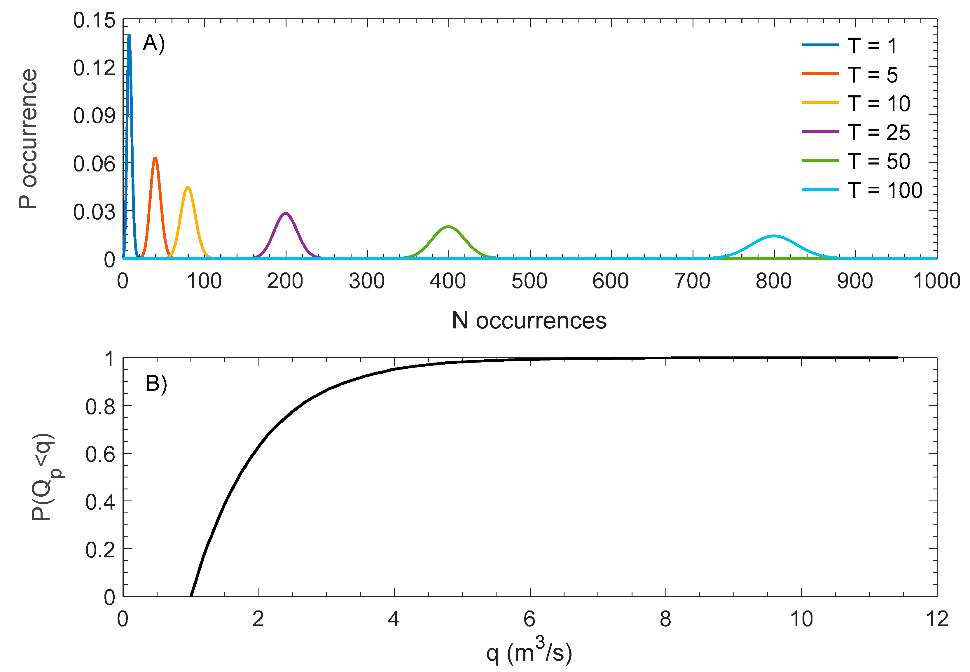
2.2. Hydrologic and Hydraulic Analysis
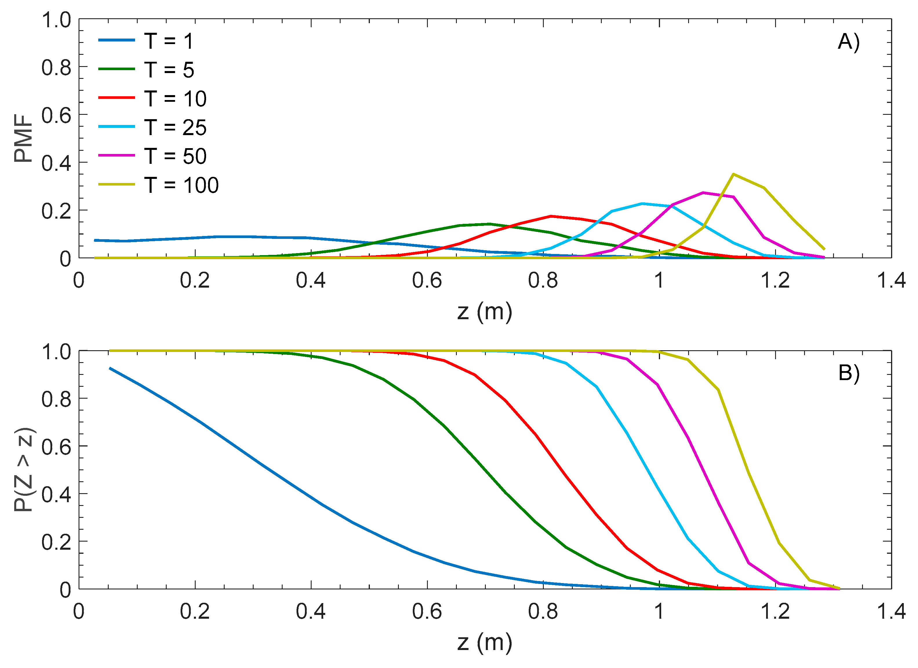
2.3. Scour Analysis
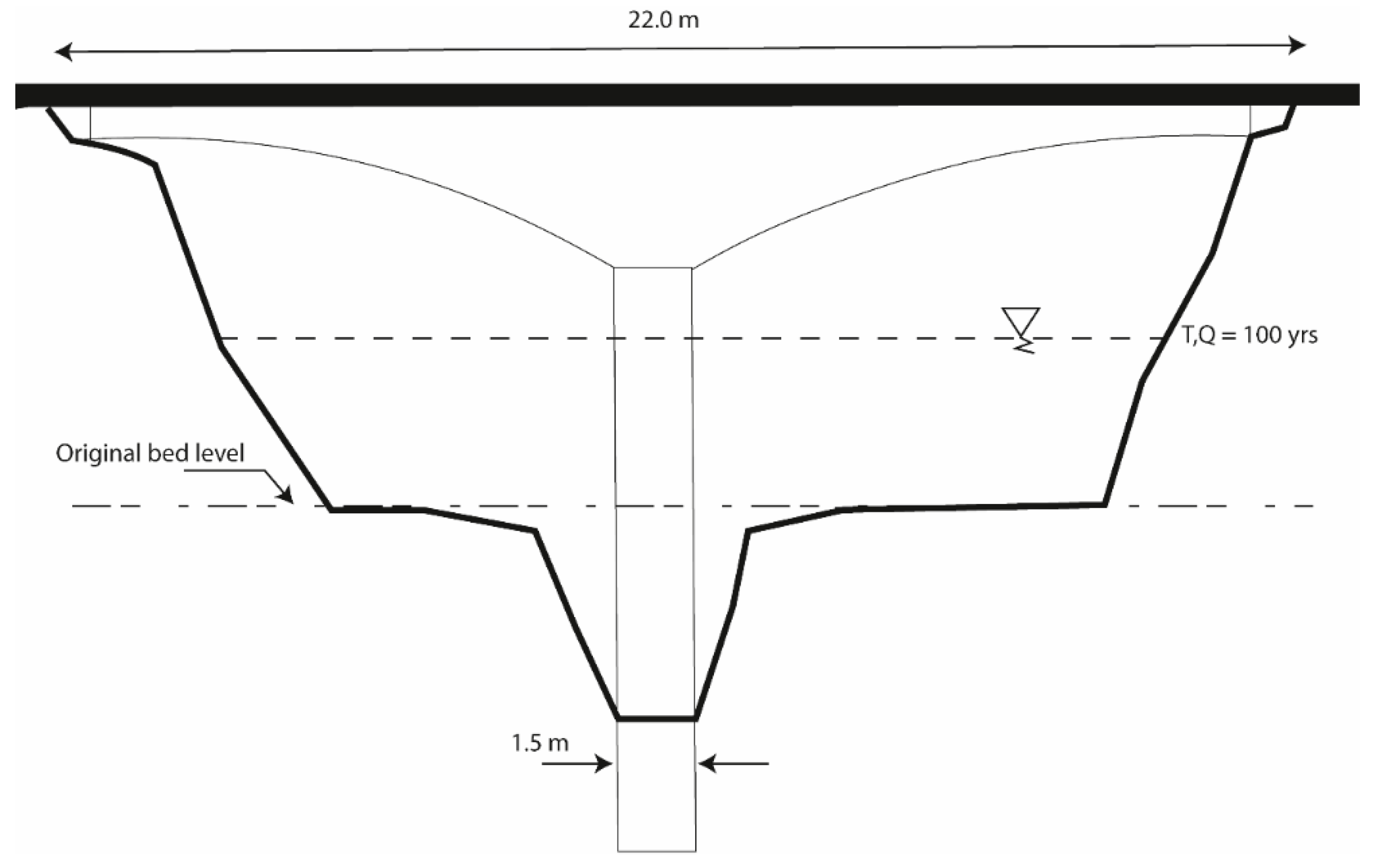
3. Case Study
4. Influence of Hydrograph Shape and Model for Describing the Temporal Evolution of Scour
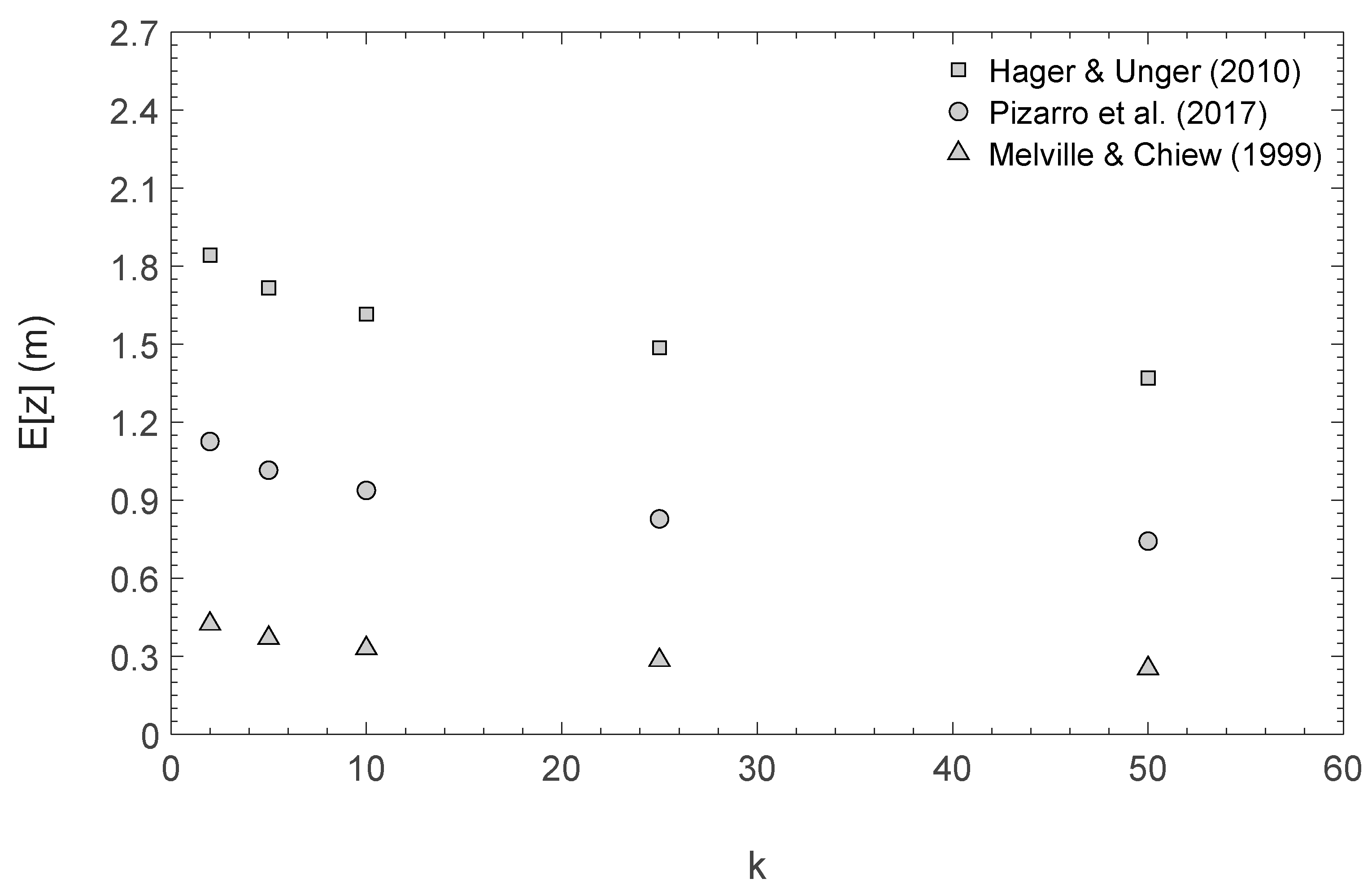
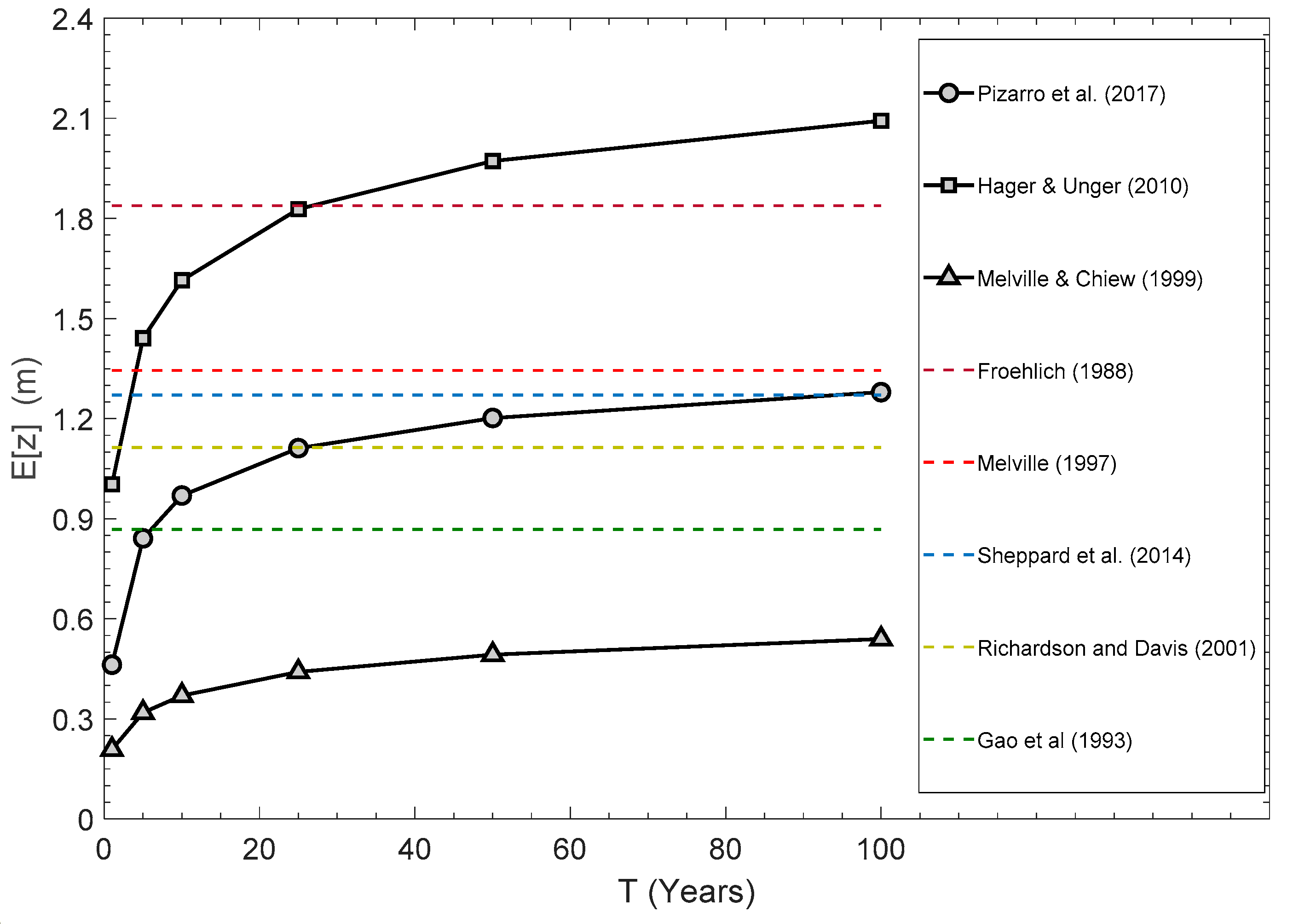
5. Comparisons with Estimates Based on Equilibrium Scour
6. Conclusions
Author Contributions
Funding
Conflicts of Interest
References
- Briaud, J.L.; Brandimarte, L.; Wang, J.; D’Odorico, P. Probability of scour depth exceedance owing to hydrologic uncertainty. Georisk 2007, 1, 77–88. [Google Scholar] [CrossRef]
- Cook, W. Bridge failure rates, consequences, and predictive trends. Ph.D. Thesis, Utah State University, Logan, UT, USA, May 2014. [Google Scholar]
- Imam, B.M.; Marios, K. Causes and consequences of metallic bridge failures. Struct. Eng. Int. 2012, 22, 93–98. [Google Scholar] [CrossRef]
- Kattell, J.; Eriksson, M. Bridge Scour Evaluation: Screening, Analysis, & Countermeasures; USDA Forest Service, San Dimas Technology and Development Center: San Dimas, CA, USA, 1998. [Google Scholar]
- Smith, D.W. Bridge failures. In Proceedings of the Institution of Civil Engineers, London, UK, August 1976; Volume 60, pp. 367–382. [Google Scholar]
- Wardhana, K.; Hadipriono, F.C. Analysis of recent bridge failures in the United States. J. Perform. Constr. Facil. 2003, 17, 144–150. [Google Scholar] [CrossRef]
- Proske, D. Bridge Collapse Frequencies Versus Failure Probabilities; Springer: Berlin, Germany, 2018; ISBN 3319738321. [Google Scholar]
- Kirby, A.; Roca, M.; Kitchen, A.; Escarameia, M.; Chesterton, O. Manual on Scour at Bridges and Other Hydraulic Structures; CIRIA: London, UK, 2015; ISBN 0860177475. [Google Scholar]
- MOP Highways design manual 2000. Available online: http://www.vialidad.cl/areasdevialidad/manualdecarreteras/Paginas/default.aspx (accessed on 17 October 2019).
- Richardson, E.V.; Davis, S.R. Evaluating Scour at Bridges. Hydraulic Engineering Circular (HEC) No. 18; U.S. Department of Transportation Federal Highway Administration: Washington, DC, USA, 2001.
- Arneson, L.A.; Zevenbergen, L.W.; Lagasse, P.F.; Clopper, P.E. Evaluating Scour at Bridges (Hydraulic Engineering Circular No. 18); US DOT: Washington, DC, USA, April 2012. [Google Scholar]
- Melville, B.W.; Coleman, S.E. Bridge Scour; Water Resources Publication: Highlands Ranch, CO, USA, 2000; ISBN 1887201181. [Google Scholar]
- TSO UK Design Manual for Roads and Bridges UK Roads Liaison Group: Background Briefing on Highway Bridges; Chartered Institution of Highways & Transportation: London, UK, 2009.
- Hamill, L. Bridge Hydraulics; CRC Press: Boca raton, FL, USA, 2014; ISBN 148227163X. [Google Scholar]
- Koutsoyiannis, D.; Montanari, A. Statistical analysis of hydroclimatic time series: Uncertainty and insights. Water Resour. Res. 2007, 43. [Google Scholar] [CrossRef]
- Dimitriadis, P. Hurst-Kolmogorov dynamics in Hydrometeorological processes and in the microscale of turbulence. Ph.D. Thesis, National Technical University of Athens, Athens, Greece, December 2017. [Google Scholar]
- Markonis, Y.; Moustakis, Y.; Nasika, C.; Sychova, P.; Dimitriadis, P.; Hanel, M.; Máca, P.; Papalexiou, S.M. Global estimation of long-term persistence in annual river runoff. Adv. Water Resour. 2018, 113, 1–12. [Google Scholar] [CrossRef]
- Koutsoyiannis, D. HESS Opinions “A random walk on water.”. Hydrol. Earth Syst. Sci. 2010. [Google Scholar] [CrossRef]
- Barbe, D.E.; Cruise, J.F.; Singh, V.P. Probabilistic approach to local bridge pier scour. Transp. Res. Rec. 1992. Available online: http://hdl.handle.net/1969.1/164643 (accessed on 17 October 2019).
- Johnson, P.A. Reliability-based pier scour engineering. J. Hydraul. Eng. 1992, 118, 1344–1358. [Google Scholar] [CrossRef]
- Brandimarte, L.; Montanari, A.; Briaud, J.-L.; D’Odorico, P. Stochastic flow analysis for predicting river scour of cohesive soils. J. Hydraul. Eng. 2006, 132, 493–500. [Google Scholar] [CrossRef]
- Kwak, K.; Briaud, J.L.; Chen, H.C. SRICOS: Computer program for bridge pier scour. Proceedings of The International Conference on Soil Mechanics and Geotechnical Engineering; Aa Balkema Publishers: Rotterdam, The Netherlands, 2001; Volume 3, pp. 2235–2238. [Google Scholar]
- Johnson, P.A.; Ayyub, B.M. Assessing time—variant bridge reliability due to pier scour. J. Hydraul. Eng. 1992, 118, 887–903. [Google Scholar] [CrossRef]
- Johnson, P.A.; Hell, T.M. Bridge Scour—A Probabilistic Approach. Infrastructure 1996, 1, 24–30. [Google Scholar]
- Yanmaz, A.M.; Üstün, I. Generalized reliability model for local scour around bridge piers of various shapes. Turkish J. Eng. Environ. Sci. 2001, 25, 687–698. [Google Scholar]
- Manfreda, S.; Link, O.; Pizarro, A. A theoretically derived probability distribution of scour. Water 2018, 11, 520. [Google Scholar] [CrossRef]
- Lagasse, P.F.; Ghosn, M.; Johnson, P.A.; Zevenbergen, L.W.; Clopper, P.E. Risk-Based Approach for Bridge Scour Prediction; National Cooperative Highway Research Program Transportation Research Board National Research Council: Washington, DC, USA, 20 October 2013. [Google Scholar]
- Tubaldi, E.; Macorini, L.; Izzuddin, B.A.; Manes, C.; Laio, F. A framework for probabilistic assessment of clear-water scour around bridge piers. Struct. Saf. 2017, 69, 11–22. [Google Scholar] [CrossRef] [Green Version]
- Oliveto, G.; Hager, W.H. Temporal evolution of clear-water pier and abutment scour. J. Hydraul. Eng. 2002, 128, 811–820. [Google Scholar] [CrossRef]
- Hager, W.H.; Unger, J. Bridge pier scour under flood waves. J. Hydraul. Eng. 2010, 136, 842–847. [Google Scholar] [CrossRef]
- Melville, B.W.; Chiew, Y.-M. Time scale for local scour at bridge piers. J. Hydraul. Eng. 1999, 125, 59–65. [Google Scholar] [CrossRef]
- Link, O.; Castillo, C.; Pizarro, A.; Rojas, A.; Ettmer, B.; Escauriaza, C.; Manfreda, S. A model of bridge pier scour during flood waves. J. Hydraul. Res. 2017, 55. [Google Scholar] [CrossRef]
- Pizarro, A.; Samela, C.; Fiorentino, M.; Link, O.; Manfreda, S. BRISENT: An Entropy-Based Model for Bridge-Pier Scour Estimation under Complex Hydraulic Scenarios. Water 2017, 11, 889. [Google Scholar] [CrossRef]
- Pizarro, A.; Ettmer, B.; Manfreda, S.; Rojas, A.; Link, O. Dimensionless Effective Flow Work for Estimation of Pier Scour Caused by Flood Waves. J. Hydraul. Eng. 2017. [Google Scholar] [CrossRef]
- Manning, R. On the Flow of Water in Open Channels and Pipes. Trans. Inst. Civ. Eng. Irel. 1891, 20, 161–207. [Google Scholar]
- Salas, J.D.; Maidment, D. Handbook of Hydrology. In Analysis and Modeling of Hydrologic Time Series; McGraw-Hill Book Co.: New York, NY, USA, 1993. [Google Scholar]
- Rogger, M.; Kohl, B.; Pirkl, H.; Viglione, A.; Komma, J.; Kirnbauer, R.; Merz, R.; Blöschl, G. Runoff models and flood frequency statistics for design flood estimation in Austria–Do they tell a consistent story? J. Hydrol. 2012, 456, 30–43. [Google Scholar] [CrossRef]
- Kothyari, U.C.; Garde, R.C.J.; Ranga Raju, K.G. Temporal variation of scour around circular bridge piers. J. Hydraul. Eng. 1992, 118, 1091–1106. [Google Scholar] [CrossRef]
- Chang, W.-Y.; Lai, J.-S.; Yen, C.-L. Evolution of scour depth at circular bridge piers. J. Hydraul. Eng. 2004, 130, 905–913. [Google Scholar] [CrossRef]
- Froehlich, D.C. Analysis of onsite measurements of scour at piers. In Hydraulic Engineering: Proceedings of the 1988 National Conference on Hydraulic Engineering, New York, NY, USA, 8–12 August 1988; ASCE: New York, NY, USA, 1988; pp. 534–539. [Google Scholar]
- Melville, B.W. Pier and abutment scour: Integrated approach. J. Hydraul. Eng. 1997, 123, 125–136. [Google Scholar] [CrossRef]
- Sheppard, D.M.; Melville, B.; Demir, H. Evaluation of existing equations for local scour at bridge piers. J. Hydraul. Eng. 2014, 140, 14–23. [Google Scholar] [CrossRef]
- Gao, D.; Pasada, L.; Nordin, C.F. Pier Scour Equations Used in the Peoples Republic of China; FHWA-SA-93-076; US Department of Transportation: Washington, DC, USA, 1993.
- Sheppard, D.M.; Melville, B. Scour at wide Piers and Long Skewed Piers. In Scour at wide Piers and Long Skewed Piers; NCHRP Report 682; Transp. Res. Board Natl. Acad.: Washington, DC, USA, March 2011. [Google Scholar]
- Johnson, P.A.; Torrico, E.F. Scour Around Wide Piers in Shallow Water. Transp. Res. Rec. 1994, 1471, 66–70. [Google Scholar]
- MATLAB, R2019a; MathWorks: Netik, MA, USA, 2019; [Computer software].
- Cunderlik, J.M.; Ouarda, T.B.M.J. Regional flood-duration—Frequency modeling in the changing environment. J. Hydrol. 2006, 318, 276–291. [Google Scholar] [CrossRef]


| Authors | Mathematical Expression | Observations | Eq. N° |
|---|---|---|---|
| Melville and Chiew [31] | Subscript “eq” means equilibrium. | (6) | |
| Hager and Unger [30] | Subscript “M” means at maximum or peak conditions. | (7) | |
| Pizarro et al. [33] | (8) |
| Authors | Mathematical Expression | Observations | Eq. N° |
|---|---|---|---|
| Froehlich [40] | = Projected width of pier. = flow depth. = Froude number. = Factor for pier shape. | (9) | |
| Melville [41] | = Factor for angle of attack. | (10) | |
| Sheppard et al. [42] | (11) | ||
| Richardson and Davis [10] | = Factor for mode of sediment transport. = Factor for armouring by bed material. = Factor for very wide piers after Johnson and Torrico [45]. | (12) | |
| Gao et al. [43] | = Incipient velocity for local scour at a pier. = Shape and alignment factor. | (13) |
| k | Hager & Unger [30] z1/ z1(k = 2) | Pizarro et al. [33] z2/ z1(k = 2) | Melville & Chiew [31] z3/ z1(k = 2) | (z1-z3) / z1(k = 2) % |
|---|---|---|---|---|
| 2 | 1.00 | 0.61 | 0.23 | 77.2 |
| 5 | 0.93 | 0.55 | 0.20 | 73.4 |
| 10 | 0.88 | 0.51 | 0.18 | 70.1 |
| 25 | 0.81 | 0.45 | 0.15 | 65.8 |
| 50 | 0.74 | 0.40 | 0.14 | 60.9 |
| Equilibrium Equation | ZEq (m) | P(Z > z) | ||
|---|---|---|---|---|
| Melville and Chiew [31] | Pizarro et al. [33] | Hager and Unger [30] | ||
| Froehlich [40] | 1.84 | 0% | 0% | 95% |
| Gao et al. [43] | 0.87 | 0% | 100% | 100% |
| Melville [41] | 1.34 | 0% | 33% | 100% |
| Richardson and Davis [10] | 1.11 | 0% | 100% | 100% |
| Sheppard et al. [42] | 1.27 | 0% | 76% | 100% |
© 2019 by the authors. Licensee MDPI, Basel, Switzerland. This article is an open access article distributed under the terms and conditions of the Creative Commons Attribution (CC BY) license (http://creativecommons.org/licenses/by/4.0/).
Share and Cite
Pizarro, A.; Tubaldi, E. Quantification of Modelling Uncertainties in Bridge Scour Risk Assessment under Multiple Flood Events. Geosciences 2019, 9, 445. https://doi.org/10.3390/geosciences9100445
Pizarro A, Tubaldi E. Quantification of Modelling Uncertainties in Bridge Scour Risk Assessment under Multiple Flood Events. Geosciences. 2019; 9(10):445. https://doi.org/10.3390/geosciences9100445
Chicago/Turabian StylePizarro, Alonso, and Enrico Tubaldi. 2019. "Quantification of Modelling Uncertainties in Bridge Scour Risk Assessment under Multiple Flood Events" Geosciences 9, no. 10: 445. https://doi.org/10.3390/geosciences9100445
APA StylePizarro, A., & Tubaldi, E. (2019). Quantification of Modelling Uncertainties in Bridge Scour Risk Assessment under Multiple Flood Events. Geosciences, 9(10), 445. https://doi.org/10.3390/geosciences9100445