Assessment of the Carbon Stock in Pine Plantations in Southern Spain through ALS Data and K-Nearest Neighbor Algorithm Based Models

Abstract

Accurate estimation of forest biomass to enable the mapping of forest C stocks over large areas is of considerable interest nowadays. Airborne laser scanning (ALS) systems bring a new perspective to forest inventories and subsequent biomass estimation. The objective of this research was to combine growth models used to update old inventory data to a reference year, low-density ALS data, and k-nearest neighbor (kNN) algorithm Random Forest to conduct biomass inventories aimed at estimating the C sequestration capacity in large Pinus plantations. We obtained a C stock in biomass (W_t-S) of 12.57 Mg·ha⁻¹, ranging significantly from 19.93 Mg·ha⁻¹ for P. halepensis to 49.05 Mg·ha⁻¹ for P. nigra, and a soil organic C stock of the composite soil samples (0–40 cm) ranging from 20.41 Mg·ha⁻¹ in P. sylvestris to 37.32 Mg·ha⁻¹ in P. halepensis. When generalizing these data to the whole area, we obtained an overall C-stock value of 48.01 MgC·ha⁻¹, ranging from 23.96 MgC·ha⁻¹ for P. halepensis to 58.09 MgC·ha⁻¹ for P. nigra. Considering the mean value of the on-site C stock, the study area sustains 1,289,604 Mg per hectare (corresponding to 4,732,869 Mg CO₂), with a net increase of 4.79 Mg·ha⁻¹·year⁻¹. Such C cartography can help forest managers to improve forest silviculture with regard to C sequestration and, thus, climate change mitigation.

1. Introduction

Forest ecosystems, covering 31% of the total land area globally, can help to mitigate the effects of climate change since carbon (C) is retained in phytomass through photosynthesis [1]. The world’s forest C stock was estimated to be 861 Pg C in 2011; biomass was the second major pool, representing 42% of this total amount [2]. At the global scale, approximately 80% of the total C contained in aboveground vegetation biomass is held in forests [3]. In the Mediterranean region, between 0.01 and 1.08 MgC·ha⁻¹ are sequestered in forest ecosystems annually [4]. For Spain, this means that around 19% of total CO₂ emissions are fixed by forests [5].

In addition to biomass, C is also stored in litter and forest soils. In fact, soils are the largest reservoir of terrestrial C, for both organic and inorganic forms [6]. Soil organic carbon (SOC) can be stored in soils for thousands of years under, suitable conditions, and is a vital component of plant nutrient cycles [7]. Forest management aimed at increasing stand growth has been shown to be effective in increasing the C sequestration capacity [8,9]. Thinning treatments improve health and tree vigor, increasing forest productivity [10], while the soil C content shows a slight decrease in the first stages, recovering its level and increasing once the canopy is restored [11].

Accurate estimation of forest biomass to produce spatially explicit mapping of forest C stocks over large study areas is of considerable interest nowadays [12]. In this regard, the field-based inventory is the most common method for evaluating the dendrometric characteristics and stand dynamics of forests. These classic forest inventories have a high demand for labor, are expensive, and require lots of field plots to obtain full inventory data for large areas on the ground [13,14]. Thus, with the advances in remote sensing techniques, these traditional methods are being replaced or supplemented with Light Detection and Ranging (LiDAR) techniques, which provide stand data over large areas, optimizing time and costs. LiDAR technology brings a new perspective to forest inventories by directly providing three-dimensional information on the entire surface [12].

LiDAR (Laser Imaging Detection and Ranging) systems from an airborne platform (airborne laser scanning, ALS) are equipped with a scanning device that distributes the emitted pulse across a swath width along the aircraft’s flight path [15]. ALS is currently considered a very useful technique for forest-characteristics estimation in both small- and large-scale studies and in different applications [14,16,17,18]. The main advantage of ALS is its ability to return forest vertical structure measurements directly, including tree crown heights, the topography of the sub-canopies, and the vertical distribution of intercepted surfaces (e.g., undergrowth). This large amount of data helps forest characterization and returns quantitative information to support forest management of large areas [19,20]. This is possible due to the strong relationship between these direct measurements and dendrometric parameters of forest stands, such as aboveground biomass and, thus, C content. By using ALS data, it is possible to produce qualitative and quantitative information about the function and productivity of forest areas. However, the use of ALS data also has limitations, like the high flight costs and the time lag between field data acquisition and the ALS flight date. In addition, commercial airborne lasers are only now becoming available on a cost-effective basis [15]. By using these techniques, forest attributes such as basal area, height, and tree diameter can be estimated using modelling algorithms and ALS data [21,22]. In Spain, in 2008–2009, the National Geographic Institute (IGN) started the capture of ALS data for a large part of Spain, within the National Plan of Aerial Orthophotography (PNOA), with low-density points in most of the flights. In Andalusia, the ALS flights were conducted between 2014 and 2016 with a pulse-density range of up to 0.5 points m⁻² (http://www.juntadeandalucia.es/medioambiente/site/rediam).

Among the wide range of algorithms used to estimate forest metrics through ALS analyses found in the literature, the k-nearest neighbor (kNN) model was selected in this study. The kNN techniques are multivariate, nonparametric methods, which find a group of k mostly similar objects for an unlabeled item and use them to assign a class label to match the class of the majority of the k-similar cases during the training [23]. These techniques have been progressively applied to forest inventory and remotely sensed data in order to map production or estimate forest attributes (e.g., forest biomass and volume stock). Particularly, the combination of a forest inventory and ALS data analysis together with the kNN technique has shown satisfactory results for the estimation of aboveground biomass [24,25].

Between the 1960s and 1970s, important reforestations were carried out in Southern Spain, mainly for soil protection purposes. In particular, at Sierra de Los Filabres (hereafter abbreviated as Filabres), these forest plantations involved different coniferous species, among which stand out—for their extension—Pinus halepensis Mill., Pinus pinaster Aiton., Pinus nigra Arnold., and Pinus sylvestris L. These plantations gave rise to forests of great homogeneity, but also of notable forestry and restorative interest [26]. This area, which also has traditional forest inventories carried out over its entire extension, is presented as a potential study area to demonstrate our hypothesis. In this regard, the general objective of this study was to combine growth models (used to update old inventory data to a reference year) and low-density ALS data to conduct biomass inventories aimed at estimating the C sequestration capacity in large plantation areas. The specific objectives were the following: (i) to collect and process classic forest inventories data, to create an updated database by applying growth models/equations; (ii) to collect SOC samples in areas under different thinning treatments; (iii) to develop C estimation models, to evaluate the sequestration capacity of a large area of forest plantations by using discrete, multiple-return, low-point-density ALS data; and (iv) to map the distribution of sequestered C as a basis for forestry management and systems optimization. The results are discussed in the context of adaptive forest management, using airborne ALS systems to monitor forest C stocks, and emission-reduction programs.

2. Materials and Methods

2.1. Study Area

The study area was located at Filabres (Andalusia region, Almería, Southeastern Spain, 37°22′ N, 2°50′ W; around 45,000 ha between 750 and 2168 m.a.s.l; Figure S1, Supplementary Materials). The mean annual precipitation is around 320 mm, while the monthly temperature oscillates between 7 and 16 °C. Present thermotypes range from the thermo-Mediterranean (below approximately 350 m) to the oro-Mediterranean, for the highest areas. The dominant soils are xerorthents regosols, mainly developed on schists and quartzites, with steep slopes (>35%) as the predominant topography [27]. The current vegetation shows a marked altitudinal gradient and is strongly influenced by reforestation programs carried out between 1955 and 1983. The most commonly used species were pines, including Pinus halepensis, P. pinaster, P. nigra, and P. sylvestris. Despite this regular plantation pattern, some reduced areas of native pine stands still exist in the area. Within Filabres, our study focused on forests owned by the Andalusia Forest Service, where most forest inventories were conducted (Figure S1. Supplementary Materials).

Our study used several data sets and required the development of remote sensing indices and data analysis procedures. Therefore, a flowchart outlining the steps and relationships of each process is provided in Figure 1.

2.2. Biomass Data

Dendrometric data were obtained from 2302 inventory plots measured in 2007, from both National Forest Inventory (IFN3) [28] and Forest Management Plans of Filabres public forests. In terms of species, there were 789, 740, 665 and 108 plots for P. halepensis, P. pinaster, P. nigra, and P. sylvestris, respectively. We considered all plots with a radius of 12.6 m and slope correction. In addition, the plot radius was used to generate vector files to divide the normalized LiDAR data, so that point clouds referring to each inventory plot were obtained. In this regard, coherence in the point clouds is needed so that their metrics are comparable and, thus, the subsequent statistical models are more robust.

In order to compare the ALS metrics with the dendrometric variables, tree diameter and height were updated to the ALS flight date (2014) by using the equations of Guzmán Álvarez et al. [29] (Equations (1) to (3)):

ln(d_i) = C₁ + C₂+ C₃ ln(N_i)+ C₄ IC_i

(1)

ln(H_i) = C₅ + C₆ ln(E_i)+ C₇ ln(IS)

(2)

where d_i is the diameter at breast height (dbh) in cm, Ni is the density (trees·ha⁻¹), IC_i is the competition index, H_i is the tree height (m), E_i is the tree age, all referred to diameter class i, C_1–7 are coefficients depending on the species and IS the site index. This index was obtained in raster format from the REDIAM data server (http://descargasrediam.cica.es/repo/s/RUR). ICi (in Equation (3)) is defined as a competition index (independent of the distance) that considered as competitors all individuals from diameter class i of the same species present in the plot, including the rest of the individuals of other species:

$${IC}_{\mathrm{i}}={\mathrm{d}}_{\mathrm{a}}·{\mathrm{N}}_{\mathrm{a}}+{{\displaystyle \sum }}_{j = 1, j \ne 1}^{Nc}{d}_{\mathrm{j}}\_N_j$$

(3)

where d_a and N_a are, respectively, the mean diameter at breast height (cm) and the total density (trees·ha⁻¹) of other species present in the plot, while d_j and N_j are, respectively, the diameter and density corresponding to the diameter class, j, of the analyzed species, where j is different from i, and Nc is the total number of diametric classes. In order to calculate this index, the plots were divided in different groups depending on the number of species present.

Given the costly procedure for updating IC, it was decided to assign a fixed value equal to the 2008 update. This is justified because this index is calculated with field inventory data, with relative centimeter-scale errors. The variation caused by the IC factor within the diameter equation ranges from precision values of hundredths to thousandths of a centimeter. Finally, the tree height and diameter of each diametric class and year were calculated for each species according to the expressions shown in Table S1 (Supplementary Materials). The tree age in the first update year (2007) was needed to start the data update for further calculation of tree height and, subsequently, tree diameter, and was inferred from previous equations (Table S1. Supplementary Materials), once the diameter and density were known from the inventory data.

The updated tree diameter and height data were used to estimate total biomass (W_t) as the sum of the biomass fractions (W_a = aboveground; W_r = root biomass), using equations from Ruiz-Peinado et al. [30] (Table S1. Supplementary Materials). Finally, a standard biomass/C coefficient of 0.5 was applied to obtain the overall C stock in biomass (W_t-S) [31]. All calculations were made for 5 cm diameter classes between 10 and >70 cm.

2.3. SOC Data

In July 2017, 36 soil point survey samples per species were taken systematically using a steel auger that was 8 cm in diameter and transported to the laboratory undisturbed. In the laboratory, all the soil soundings were cut into four sections: 0–10, 10–20, 20–30, and 30–40 cm, in the first part of the mineral soil. All the soil samples were air-dried, and then coarse particles were removed with a sieve (mesh size 2 mm); the resultant fine-earth fraction was ground to pass through a 0.5 mm mesh and stored for SOC determination. In the sieving process, all particulate organic matter (rootlets, leaves, seeds, and other plant material) was manually extracted. The gravel (>2 mm) was weighed and stored separately. For each soil sample, three replicates of each measurement were performed in the laboratory.

The organic carbon content of the fine-earth was determined through wet oxidation by the Walkley and Black method [32]. The bulk density (BD) of fine-earth in every soil layer was estimated as follows (g·cm⁻³) (Equation (4)):

BD = W_(fe)/(Vol_cil. − (W_(gr)/BD_(gr))

(4)

where W_(fe) is the weight of fine-earth fraction, Vol_cil. is the volume of the cylinder (10 cm height), W_(gr) is the weight of gravel fraction and, BD_(gr) is the bulk density of the gravels, obtained in every case by the quotient between the weight of gravels ant its volume obtained by the displacement of water.

The soil organic carbon stock (SOC-S, Mg·ha⁻¹) was computed for each layer and expressed in kg·m⁻², by Equation (5) [33,34]:

SOC-S = (SOC/100) × BD × C_m × D × 10

(5)

where SOC is soil organic carbon concentration, in weight percent (%), BD is bulk density of fine-earth (g·cm⁻³), D is thickness of the analyzed layer (cm), and 10 is the factor for conversion from g/cm³ to kg/m². C_m is the fraction of the volume occupied by fine-earth, obtained from Equation (6):

C_m = Vol_<2mm/Vol_whole = (%_(fe)/BD_(fe))/(%_(fe)/BD_(fe) + %_(gr)/BD_(gr))

(6)

where %_(fe) is the fine-earth percentage, BD_(fe) is the bulk density of fine-earth, %_(gr) is the gravels percentage, and BD_(gr) is the bulk density of gravels. The overall soil organic carbon stock (SOC₄₀-S) in the first 40 cm from the soil surface was calculated by adding together the values obtained for each layer. A sub-meter global satellite receiver (Leica Zeno 20 GIS, Leica Geosystems, Switzerland) was used to survey plot centers and soil samples.

2.4. ALS Data and Processing

Low-density ALS data were provided by the PNOA (http://pnoa.ign.es/presentacion) through the IGN website. The objective of the LiDAR-PNOA project is to cover the entire Spanish national territory in point clouds with X, Y, and Z coordinates obtained by airborne ALS sensors, with a density of 0.5 points m⁻² and altimetric accuracy better than 20 cm. In our study area, the ALS flight was performed in 2014. Data were provided in 2 km × 2 km tiles of raw data points in a LAZ binary file (compressed LAS files), containing x and y coordinates (EPSG: 25,830 ETRS 1989/UTM Zone 30) and ellipsoidal elevation Z. The ALS data were processed in FUSION LDV 3.80 [35]. Before starting the work, the LAZ files were decompressed using the Laszip command from the LAStools software [36], to obtain the LAS files. Due to the large extension of the study area, all files were divided in different lots, so the software could handle the heavily normalized surface files obtained throughout the process. The working flow, using FUSION commands to process and normalize ALS data, is shown below, in order of execution.

In summary, the ALS point clouds were first filtered to generate a surface model (cell size 0.5 m), and ALS metrics were computed for each inventory plot after normalizing the data by subtracting the DTM from the point clouds [37]. Finally, 2302 metrics records were obtained, including 99 statistical parameters for each one. Before implementing the analyses, statistical parameters without forest significance were deleted (mainly intensity-derived parameters) [38]. Finally, 50 out of the 99 original parameters were used as regressors, including the mean, maximum, and minimum values, mode, standard deviation, variance, interquartile distance, coefficients of skewness and kurtosis, average absolute deviation, and percentiles. In addition, the percentage of returns above 2 m (above this height is considered canopy), mean, and mode were selected (Table S2. Supplementary Materials).

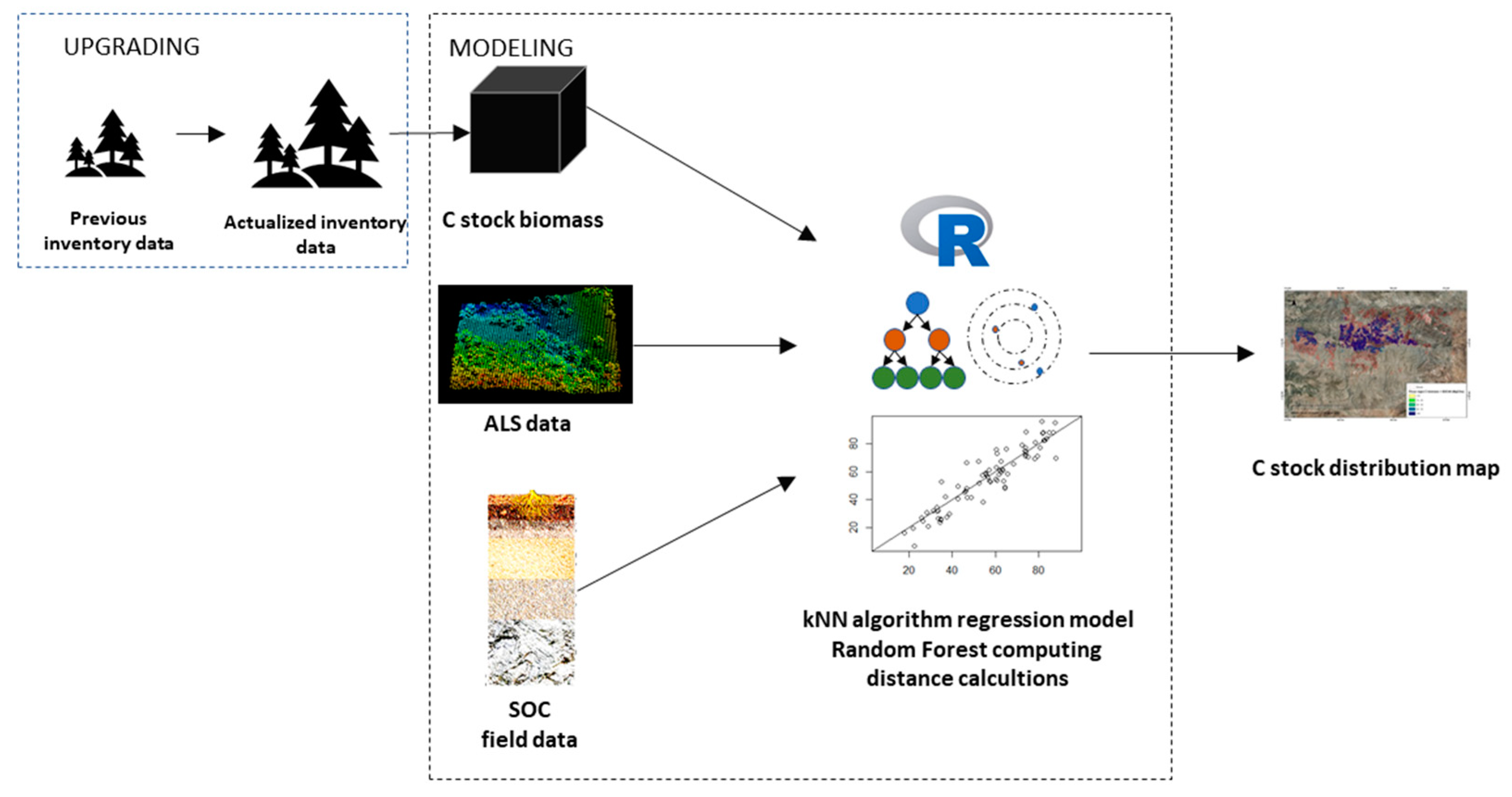
2.5. Data Analysis and kNN Models

A spatial C-stock model depending on ALS metrics was determined using the k-nearest neighbor (kNN) machine-learning algorithm, in particular using a random forest (RF) model. [25]. When using this model, no assumption regarding the nature of the data is required (e.g., normality or homoscedasticity) [25]. In terms of the relationships among variables, multicollinear explanatory variables may alter their effects on the model response due to either true synergistic relationships among the variables or false correlations. Due to this and prior to variables selection, variance inflation factor (VIF) analysis was conducted to check multicollinearity among preselected variables (Table S2. Supplementary Materials).

From these previous analyses, 13 ALS variables with little correlation among themselves were selected (listed in order of significance): all returns above mode/total first returns * 100, percentage of all returns above mode, elevation maximum, elevation mode, elevation MAD mode (median of the absolute deviations from the overall mode), elevation L CV (coefficient of variation for cell of elevation L-moment), elevation kurtosis (kurtosis computed for cell), return 1 count (count of return 1 points above 2 m), elevation MAD median (median of the absolute deviations from the overall median), percentage all returns above mean, elevation minimum, percentage all returns above 2 m, and return 2 count (count of return 2 points above 2 m). For complete information about the statistical parameters, see McGaughey [35].

In order to validate the estimations of the models, the input data were separated into training and evaluation sets, covering 70% and 30% of the input data, respectively. Later, the variable selection process was executed by choosing the combination of variables that minimized the generalized root mean square distance when variables were added or deleted one at a time [38,39]. Once the best predictor variables were selected, we used random forest (RF) to model the C stock in biomass (per species) and the soil organic carbon stock (SOC₄₀-S) (for all Pinus species together) [40]. We assessed the model accuracy through internal validation, including a Q-value overfitting test. External validation and cross-validation were then run. The RMSE and bias were calculated for each process. Finally, raster files for W_t, SOC₄₀-S and W_t + SOC₄₀-S were obtained. Each pixel represents the mean value for the on-site C stock (Mg·ha⁻¹) as a function of the selected independent ALS variables.

All statistical analyses were performed with R software [41], version 3.5.1. The usdm package [42] was used to perform multicollinearity analysis, while variables selection and regression with kNN were run with the yaImpute R package [38].

2.6. Quantification and Cartography of C Stocks

A C stock map of the on-site C stock, including the total C stock in biomass (W_t-S) and the SOC stock of the composite soil samples (0–40 cm, SOC₄₀-S), for each pine species, was developed. The original raster was reclassified in six different classes, according to the C content per hectare, using the SAGA Reclassify Grid Values Module (v2.2.5). The pixel size selected to compute the ALS metrics, and thus to generate the C stock cartography, was 22.3 × 22.3 m, representing a pixel surface area similar to the field plots surface area (Equation (7)):

$$\mathrm{cell}\mathrm{size}=\mathsf{\surd }\left(\mathrm{field}\mathrm{plot}\mathrm{surface}\mathrm{area}\right).$$

(7)

The total C stock sequestered in the Filabres plantations was estimated by using the mean value of Mg·ha⁻¹ and the total raster surface area. This surface area was calculated considering the pixel surface area and the total number of pixels, using the r.report GRASS algorithm for QGIS. The original raster files obtained directly from the RF kNN model were improved through the r.neighbors GRASS algorithm and reclassified in five different classes according to the C content per hectare (<10, 10–20, 20–30, 30–40, and >40 MgC·ha⁻¹). The SAGA Reclassify grid values tool for QGIS was used for this purpose.

3. Results

3.1. C Stocks in Biomass and SOC by Species

Table 1. Silvicultural characteristics, C stock in live-biomass and soil organic carbon stocks (Mg·ha⁻¹) of Pinus sp. plantations at Sierra de los Filabres (Almería, Southern Spain). Variables and abbreviations: stem density (N, trees·ha⁻¹); Assman’s dominant height (H_o, m); quadratic mean diameter (D_g, cm); basal area (G, m²·ha⁻¹); C stock in biomass (W_t, Mg·ha⁻¹) and soil organic carbon stock (SOC_depth-S, Mg·ha⁻¹). Values are means ± SE. Different letters indicate significant post hoc differences between thinning treatments at alpha = 0.05, based on a one-way ANOVA.

	Pinus Halepensis	Pinus Nigra	Pinus Sylvestris	Pinus Pinaster
Surface area (ha)	9118	7507	5900	5658
Dg (cm)	17.57 (0.26)b	18.45 (0.16)b	17.94 (0.32)b	23.75 (0.21)a
BA (m2·ha−1)	10.19 (0.33)c	19.48 (0.50)b	14.41 (1.09)c	24.02 (0.62)a
N (trees·ha−1)	419.32 (10.88)c	732.35 (18.23)a	605.04 (48.29)b	536.81 (12.93)b
Ho (m)	9.10 (0.12)c	9.49 (0.11)b	8.92 (0.18)c	11.30 (0.09)a
Wt (Mg·ha−1)	19.93 (0.75)c	49.05 (1.40)a	35.23 (2.65)b	43.49 (1.19)a
SOC10 (Mg·ha−1)	10.51 (0.57)a	5.88 (0.69)b	6.15 (0.58)b	10.10 (0.75)a
SOC40 (Mg·ha−1)	37.32 (2.24)a	24.50 (1.49)a	20.41 (2.18)a	34.14 (2.29)a
Wt + SOC40 (Mg·ha−1)	57.25 (1.41)c	73.55 (1.29)a	55.64 (2.01)b	77.63 (2.12)a

shows the values of silvicultural characteristics, after updating dendrometric data from 2007 to 2014, W_t-S and SOC-S of the Pinus sp. plantations at Sierra de los Filabres. Pinus pinaster was the species with the highest height and diameter values, followed by P. nigra. Pinus sylvestris showed the lowest values, although the plantation of this species was set up in the same years. The W_t-S derived from the dendrometric data ranged significantly from 19.93 Mg·ha⁻¹ for P. halepensis to 49.05 Mg·ha⁻¹ for P. nigra (F = 295.63, P < 0.001), with an average value of 36.92 Mg·ha⁻¹.

Our estimate of SOC shows a large C stock in the mineral soils, with nonsignificant differences in SOC-S between species (Table 1, F = 1.95, P = 0.329). The SOC₄₀-S values of the composite soil samples (0–40 cm) ranged from 20.41 Mg·ha⁻¹ in P. sylvestris to 37.32 Mg·ha⁻¹ in P. halepensis. The value of W_t +SOC₄₀-S was higher for P. sylvestris (77.63 Mg·ha⁻¹) and P. nigra (73.55 Mg·ha⁻¹), with significant differences (F = 177.31, P < 0.001, Table 1). The SOC₄₀-S accounted for 65.18% of the total on-site C stock for P. halepensis and less than 50.00% for the other three species.

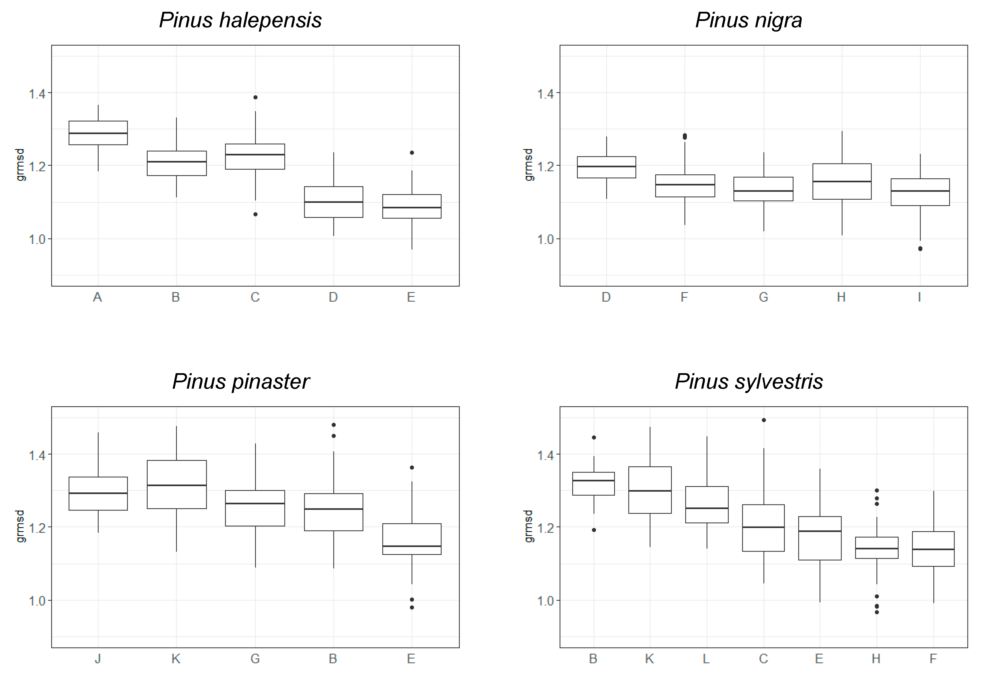
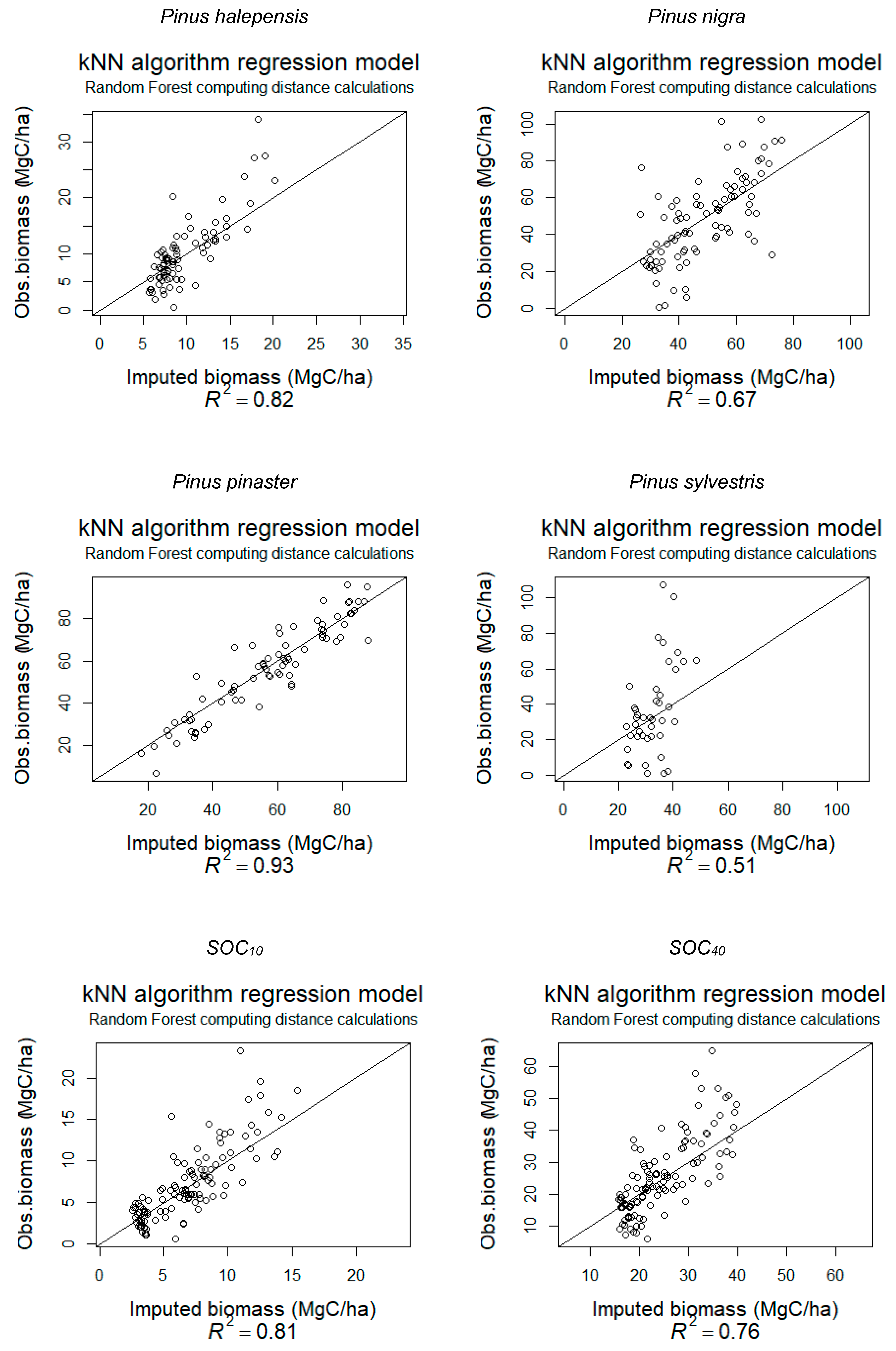
3.2. kNN Model for C Stocks Predictions

Following the selection of the independent variable data, the RF model used between five (P. halepensis) and seven (P. sylvestris) among twelve variables: Elev.P90, Elev.mode, Percentage.all.returns.above.mean, Elev.kurtosis, Elev.MAD.median, Return.1.count, Elev.minimum, H: Percentage.all.returns.above.mode, Elev.maximum, Canopy.relief.ratio, Elev.P99 and Return.2.count. (Figure 2; Table S2. Supplementary Materials). We computed the scatter plots for correlations contrasting the observed versus the estimated values for the C-stock predictions, for all species (Figure 3; Table S3. Supplementary Materials). For W_t-S, the best model was obtained for P. pinaster (R² = 0.93, RMSE = 16.56 Mg·ha⁻¹); for the other species, the fit ranged between R² = 0.82 (RMSE = 5.26 Mg·ha⁻¹) for P. halepensis and R² = 0.51 (RMSE = 33.45 Mg·ha⁻¹) for P. sylvestris. The best model prediction for SOC-S was obtained for SOC₁₀-S for all Pinus species (R² = 0.81, RMSE = 4.92 Mg·ha⁻¹), although the model prediction for SOC₄₀-S also provided a high coefficient of determination (R² = 0.76, RMSN = 12.92 Mg·ha⁻¹).

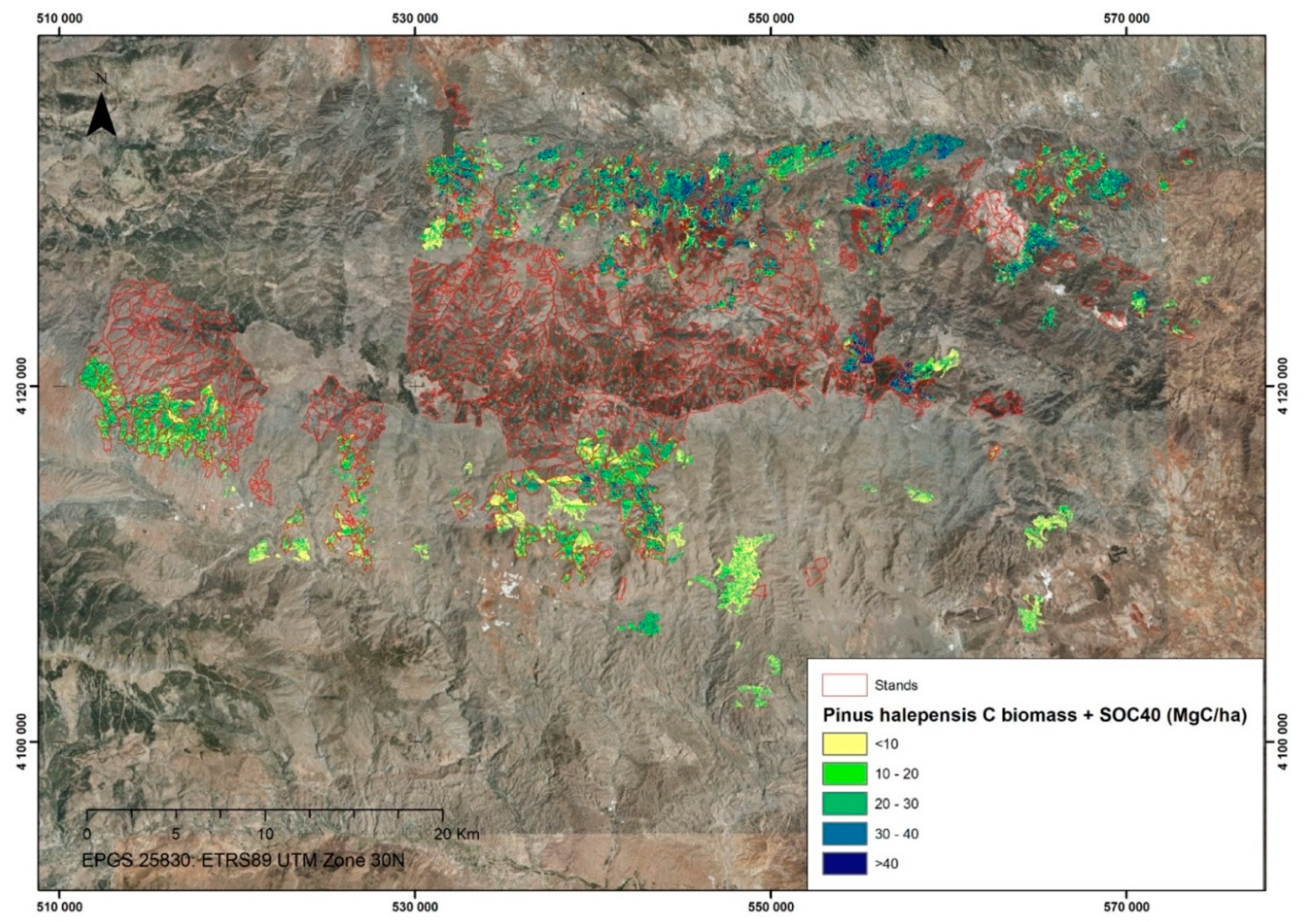
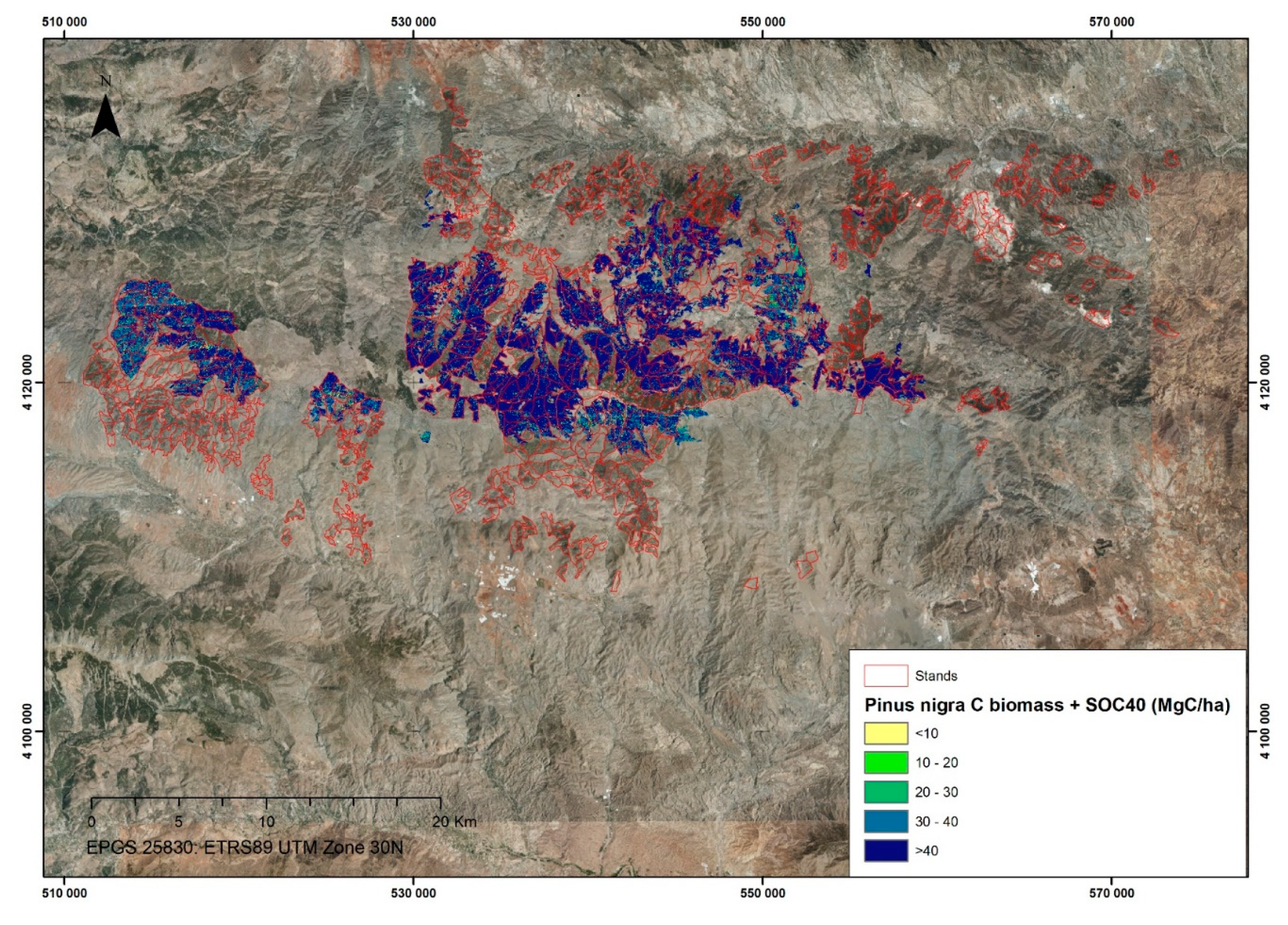
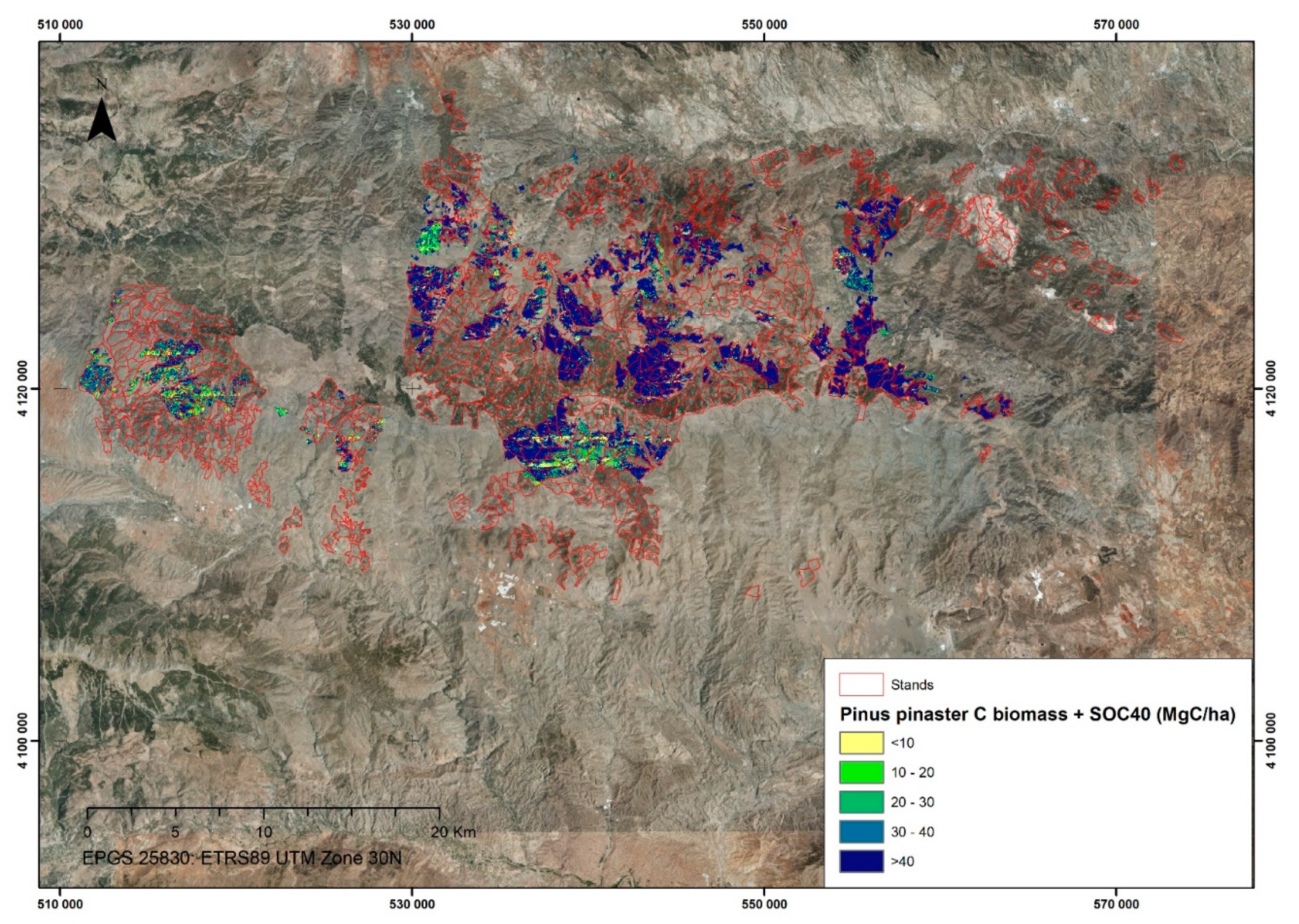
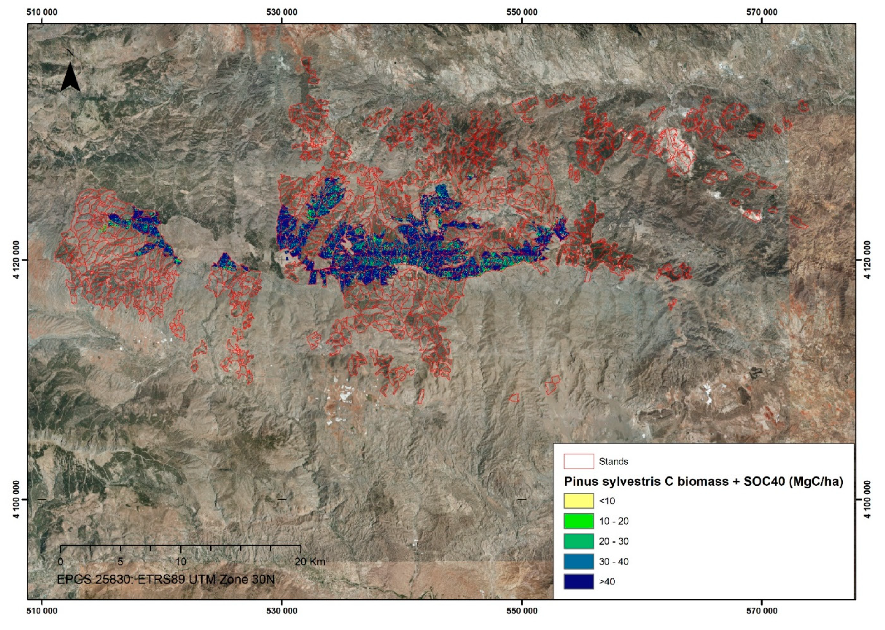
3.3. Cartography of C Stocks

Figure 4, Figure 5, Figure 6 and Figure 7 show the distribution of the overall C stocks (W_t-S + SOC₄₀-S) throughout all the Filabres forests, for P. halepensis, P. nigra, P pinaster, and P. sylvestris, respectively. We obtained a mean overall C-stock (W_t and SOC₄₀-S) value for the whole area of 48.01 Mg·ha⁻¹, ranging from 23.96 Mg·ha⁻¹ for P. halepensis to 58.09 Mg·ha⁻¹ for P. nigra. The mean W_t-S value was 31.77 Mg·ha⁻¹, ranging from 8.26 Mg·ha⁻¹, for P. halepensis to 41.97 Mg·ha⁻¹ for P. nigra. A mean SOC₄₀-S value of 16.23 Mg·ha⁻¹ was obtained—ranging from 15.70 Mg·ha⁻¹ for P. halepensis, to 17.02 Mg·ha⁻¹ for P. sylvestris (

Table 2. Stand characteristics—basal area (BA), quadratic mean diameter (D_q), number of stems (N), dominant height (H_o), C stock in live-biomass (W_t-S), and soil organic carbon stock in the 0–40 cm soil layer (SOC₄₀)—for each of the four Pinus spp.: Pinus halepensis, Pinus nigra, Pinus pinaster, and Pinus sylvestris at Sierra de los Filabres (Southern Spain). Values are means (SE).

Species		Stands	G (m2·ha−1)	Dq (cm)	Ho (m)	N (stems·ha−1)	SOC40 (Mg·ha−1)	Wt (Mg·ha−1)
Pinus halepensis	<30 ha	51	9.45 (5.52)	16.57 (2.63)	8.35 (1.48)	455.04 (193.04)	16.12 (7.81)	8.16 (5.21)
	30–40	70	9.44 (5.72)	16.47 (2.68)	8.26 (1.51)	445.01 (197.52)	15.82 (7.72)	8.52 (5.73)
	40–50	72	8.99 (5.54)	16.33 (2.68)	8.19 (1.51)	442.27 (193.96)	15.45 (7.69)	7.83 (5.10)
	50–60	49	9.13 (5.61)	16.54 (2.73)	8.27 (1.54)	443.61 (190.17)	15.64 (7.94)	8.02 (5.11)
	60–70	41	9.62 (5.76)	16.51 (2.71)	8.27 (1.52)	456.49 (198.88)	15.52 (7.81)	8.97 (6.03)
	70–80	22	9.27 (5.60)	16.42 (2.69)	8.21 (1.51)	435.41 (195.13)	15.60 (7.45)	7.73 (4.82)
	80–90	18	10.70 (6.46)	16.91 (2.77)	8.46 (1.51)	475.92 (200.53)	15.06 (7.57)	8.42 (5.49)
	90–100	6	11.61 (7.70)	17.51 (3.28)	8.80 (1.80)	459.59 (213.33)	16.74 (7.82)	9.21 (6.25)
	>100	1	16.89 (9.80)	21.20 (4.05)	10.72 (2.03)	465.27 (210.04)	22.04 (7.52)	13.54 (9.54)
Pinus nigra	<30 ha	50	12.24 (7.78)	17.78 (3.32)	8.98 (1.79)	503.48 (226.39)	16.53 (8.09)	43.32 (18.94)
	30–40	119	12.51 (7.52)	17.64 (3.16)	8.91 (1.69)	517.09 (222.59)	16.35 (8.03)	43.05 (18.40)
	40–50	110	11.43 (7.10)	17.29 (3.07)	8.72 (1.67)	494.03 (212.43)	15.99 (8.04)	41.68 (18.41)
	50–60	89	11.40 (6.89)	17.29 (3.03)	8.70 (1.65)	501.75 (214.36)	15.85 (7.87)	40.43 (17.64)
	60–70	72	11.35 (6.93)	17.27 (3.04)	8.67 (1.65)	498.44 (209.10)	15.89 (7.82)	40.54 (17.76)
	70–80	38	12.73 (7.68)	17.63 (3.16)	8.90 (1.67)	521.27 (224.39)	16.28 (7.93)	41.41 (18.48)
	80–90	22	13.13 (7.92)	17.91 (3.37)	9.02 (1.76)	531.87 (228.82)	16.34 (7.87)	46.80 (19.15)
	90–100	9	11.63 (7.27)	17.47 (3.15)	8.74 (1.69)	504.17 (228.93)	15.91 (7.75)	41.01 (17.99)
	>100	-	-	-	-	-	-	-
Pinus pinaster	<30 ha	50	12.23 (7.84)	17.74 (3.34)	8.95 (1.79)	503.33 (230.11)	16.86 (8.11)	45.19 (20.33)
	30–40	100	12.27 (7.16)	17.63 (3.12)	8.88 (1.66)	509.70 (219.97)	16.58 (7.88)	44.57 (19.22)
	40–50	90	10.78 (6.66)	17.05 (3.00)	8.58 (1.64)	482.24 (210.27)	15.60 (7.93)	40.40 (18.33)
	50–60	73	10.79 (6.60)	17.08 (2.95)	8.57 (1.61)	490.15 (211.98)	15.59 (7.81)	37.95 (17.82)
	60–70	57	11.69 (7.16)	17.39 (3.10)	8.73 (1.65)	505.11 (214.30)	16.19 (7.76)	42.34 (17.55)
	70–80	33	10.25 (6.64)	16.77 (2.90)	8.41 (1.59)	473.82 (218.81)	15.46 (7.70)	38.58 (19.03)
	80–90	16	12.74 (8.07)	18.01 (3.54)	9.05 (1.84)	510.64 (230.64)	16.75 (8.10)	49.45 (18.79)
	90–100	10	11.68 (7.40)	17.46 (3.23)	8.76 (1.73)	504.67 (229.02)	15.97 (7.76)	38.35 (19.82)
	>100	-	-	-	-	-	-	-
Pinus sylvestris	<30 ha	26	13.67 (8.67)	18.39 (3.61)	9.32 (1.90)	529.36 (239.54)	17.48 (8.41)	34.08 (23.10)
	30–40	68	14.18 (8.52)	18.30 (3.45)	9.27 (1.80)	545.13 (233.82)	17.33 (8.14)	36.43 (22.79)
	40–50	63	13.20 (8.31)	17.98 (3.44)	9.12 (1.84)	520.31 (227.37)	17.21 (8.22)	35.14 (22.51)
	50–60	56	12.25 (7.60)	17.60 (3.20)	8.90 (1.73)	523.79 (226.17)	16.25 (7.95)	32.73 (20.58)
	60–70	36	13.13 (7.92)	17.84 (3.28)	8.98 (1.71)	532.18 (221.72)	17.01 (7.70)	34.65 (21.46)
	70–80	23	14.21 (8.57)	18.04 (3.34)	9.13 (1.73)	539.97 (228.88)	16.82 (7.98)	36.08 (22.71)
	80–90	9	13.79 (8.39)	18.25 (3.65)	9.24 (1.88)	551.74 (241.43)	17.43 (8.27)	39.03 (22.26)
	90–100	4	14.69 (8.56)	18.58 (3.50)	9.34 (1.76)	565.71 (251.33)	17.32 (7.61)	31.29 (17.74)
	>100	-	-	-	-	-	-	-

).

Starting from the abovementioned results, the current on-site C stock estimated for the total forested area was 1,289,604 Mg, including 833,891 Mg in W_t-S and 455,713 Mg in SOC₄₀-S (corresponding to 4,732,869 Mg CO₂), with a net increase of more than 4.79 Mg·ha⁻¹·year⁻¹.

4. Discussion

In Spain and other Mediterranean countries, restoration efforts have been made to re-establish forest cover on landscapes previously supporting marginal forest vegetation and crops [43]. Such pine plantations are managed for multi-objective optimization: to integrate forest products and ecosystem services, such as erosion and water protection; to re-establish the native forest cover; for social uses; and, more recently, C sequestration [44]. The purpose of this study was to confirm the hypothesis that, by combining growth models, data extracted from forest inventories, and low-density ALS data, we could estimate W_t-S and SOC-S in large plantation areas through biomass models built using a kNN algorithm. As Maltamo et al. [18] also found the use of ALS data and dendrometric measurements from inventory plots greatly reduces the fieldwork required to obtain large-surface-area C models and serves as a very useful tool in the management of forest stands for C sequestration purposes. The ALS-based cartography of C stocks is an essential tool for the planning of alternative silvicultural management intended to optimize C sequestration in forests. However, the integration of SOC stocks into on-site C stocks and the sequestration rates of Mediterranean Pinus plantations remain poorly described [45]. In this study, we highlight the availability of ALS and kNN algorithms for the assessment of C stocks over large surface areas, which facilitates C-based silviculture; this complements previous research on the estimation of on-site C stocks in Mediterranean pine plantations [40].

4.1. The C Stocks in Biomass and SOC for Different Pinus sp.

Using the equations proposed by Guzmán Álvarez et al. [29] to update the tree height and diameter and those of Ruiz-Peinado et al. [30] for biomass estimation, we obtained the total W_t-S of Pinus sp. plantations at Filabres (Southern Spain). The W_t-S ranged between 19.93 Mg·ha⁻¹ for P. halepensis and 49.05 Mg·ha⁻¹ for P. nigra. These values are higher than those reported for dominant pine forests in similar ecological conditions (15.91 Mg·ha⁻¹, P. halepensis; 25.33 Mg·ha⁻¹, P. nigra; 22.33 Mg·ha⁻¹, P. pinaster; and 23.52 Mg·ha⁻¹, P. sylvestris, [29]). By species, the W_t-S were lower than those reported for dominant Aleppo pine forests in similar ecological conditions (25.29 Mg·ha⁻¹ [23]), but were closer to those of other studies (15.02 Mg·ha⁻¹ [46]; 19.93 Mg·ha⁻¹ [47]; 13.93 Mg·ha⁻¹ [40]). For P. nigra in Mediterranean locations, Vayreda et al. [47] estimated a value of 32.70 Mg·ha⁻¹, lower than that obtained in Sierra de los Filabres (49.50 Mg·ha⁻¹). In a maritime pine forest, we obtained a value (43.49 Mg·ha⁻¹) that was very similar to that reported by Vayreda et al. [47] (44.80 Mg·ha⁻¹) but lower than that calculated for other plantations (82.25 Mg·ha⁻¹ [48]) and much lower than that reported by Ruiz-Peinado et al. [49] (90 Mg·ha⁻¹). Finally, for P. sylvestris in Mediterranean locations in Northern Spain, Bravo et al. [50] and Vayreda et al. [47] estimated a W_t-S of 51.10 Mg·ha⁻¹ and 48.70 Mg·ha⁻¹, respectively, higher than that obtained in Sierra de los Filabres (35.23 Mg·ha⁻¹). These discrepancies can be explained by the structural–silvicultural heterogeneity of the pine stands in relation to age and density, as well as differences in environmental site conditions. The wide range of estimates of biomass C stock might be negatively affected by the fact that they are typically derived from general allometric equations [5]. We recognize that projection of dendrometric variables from traditional inventories is challenging, even in homogenous canopies; thus, the outcomes are biased because these models do not reflect all the variation in forest structure. If those restrictions are ignored when calculating biomass stocks, final estimates will include unpredictable increases in error. These factors determine that W_t-S values have great variation, even when compared locally [29].

Regarding the SOC stocks, SOC₄₀-S ranged from 20.41 Mg·ha⁻¹ for P. sylvestris to 37.32 Mg·ha⁻¹ for P. halepensis. These values are lower than those found in other studies, which determined the average SOC-S for a P. halepensis plantation (Northern Spain, 300 trees·ha⁻¹, dbh = 17.5 cm, 40.72 Mg·ha⁻¹ [51]; SOC-S ranged between 90 and 166 Mg·ha⁻¹ [52,53]) and for P. sylvestris (102 Mg·ha⁻¹ [1]) and P. pinaster (107 Mg·ha⁻¹ [49]). These differences may be related to the shallow soil layers (0–40 cm) in our study, which limit the SOC related to root density [54]. Additionally, the litter quantity and turnover are very limited because more of the thinning residues, such as slashes, are left on-site without crushing, thus reducing the soil C stocks [55]. Determining SOC stock in large forest areas can be difficult because of the spatial variability in SOC stock and the different measurement errors associated. To reduce these heterogeneities and uncertainties, the design of a SOC sampling strategy was planned to ensure harmonized data collection and data processing [56]. However, the overall design of SOC sampling was determined by time and budgetary availability. The overall average on-site C stock (W_t plus SOC₄₀-S) was 48.01 Mg·ha⁻¹, ranging from 23.96 Mg·ha⁻¹ for P. halepensis to 58.09 Mg·ha⁻¹ for P. nigra. Few studies have estimated the C stock for Pinus plantations [1,45,57], but they obtained higher values (ranging from 302 Mg·ha⁻¹ to 294 Mg·ha⁻¹ for P. pinaster and P. sylvestris, respectively, [49]). Navarro-Cerrillo et al. [40] obtained an average of total C stocks for P. halepensis stands in Southeastern Spain of 89.42 Mg·ha⁻¹, which is still higher than the values obtained in this study. Again, these discrepancies can be explained by the differences in soil quality and the structural–silvicultural heterogeneity, but also by the use of national allometric equations that may have limitations for their application at a local scale [58].

Despite these differences, our results support the idea that Pinus plantations in degraded semi-arid areas have an important role in the C cycle and on-site C sequestration [46]. The forest management, along the 35-year management period, had an impact on the on-site C stock (W_t + SOC₄₀-S), evidencing that Pinus plantations are more efficient in terms of C sequestration than other agricultural land uses [59,60].

4.2. The Use of ALS Data and a kNN Model for C Stocks Estimation

Here, kNN algorithms were used to generate spatially explicit forest C-stock models using ALS and inventory data [25,40,61]. We selected the RF model because it was proved to perform better than multivariate linear regression and other nonparametric statistical methods in the prediction of W_t-S [40,62].

In our study, all the species models were built with 12 ALS variables that were selected after collinearity analysis and ranked high in RF. The ALS metrics most strongly related to the C stocks in Pinus plantations were height metrics (Elev.P90, Elev.mode, Percentage.all.returns.above.mean, Elev.kurtosis, Elev.MAD.median, Elev.minimum, Percentage.all.returns.above.mode, Elev.maximum, Elev.P99), and other ALS-derived metrics concerning the horizontal distribution of the point cloud (Return.1.count, Canopy.relief.ratio, Return.2.count). Metrics generated from ALS data are commonly agreed to be highly correlated with C stocks, and many studies have successfully used height metrics (higher percentiles, mean, and maximum height) as important predictors for their quantification in Mediterranean pine species [23,40,63] and other conifers [14,64,65,66]. In our study, all the species models used similar metrics, which demonstrates the consistency of the models. Maximum height metrics (Elev.P90, Elev.P99, Elev.maximum) may be related to Ho measurements; metrics of average heights (Elev.mode, Elev.MAD.median) to measures of basal area or diameters; and pulse density metrics (Return.1.count, Return.2.count, Canopy.relief.ratio) to plot density or cover fraction.

Consistent results were obtained for model calibration, using all samples and leave-one-out cross-validation for W_t-S and SOC₄₀-S40. The best fit of the W_t-S model was obtained for P. pinaster (R² = 0.93, RMSN = 16.56 Mg·ha⁻¹), and the worst was for P. sylvestris (R² = 0.51, RMSN = 33.45 Mg·ha⁻¹). This is in accordance with other studies [62], including Montealegre et al. [23] and Navarro-Cerrillo et al. [40], who modelled the volume in P. halepensis plantations using low-density ALS data (1–0.5 points m⁻²) (R² = 0.89, RMSE = 11.01 m³·ha⁻¹) and W_t-S estimations for coniferous species (R² = 0.46 to 0.97 [23,37,67,68]). For SOC-S, the model obtained for SOC₁₀-S (R² = 0.82, RMSE = 4.92 Mg·ha⁻¹) was better than that for SOC₄₀-S (R² = 0.76, RMSE = 12.92 Mg·ha⁻¹) and similar to those found by Navarro-Cerrillo et al. [40] in similar ecological conditions. The RMSE estimations were slightly higher (with the exception of P. nigra, 93.12%) than those obtained in other studies (RMSE = 40%–44%, [69]) of W_t-S at plot-level. Navarro-Cerrillo et al. [40] obtained W_t-S models for P. halepensis stands with RMSE values ranging from 8.03 to 11.62 Mg·ha⁻¹. The difference in RMSE between models may indicate that the models were not very sensitive with regard to the differentiation of high W_t-S values, which frequently resulted in the underestimation of large W_t-S areas. However, the observed W_t-S values ranged from 19 to 49 Mg·ha⁻¹, approximately, within the range of the prediction models (with the exception of P. halepensis, for which the predicted W_t-S only reached 13 Mg·ha⁻¹), indicating good estimations of high W_t-S. Higher values of RMSE can be explained by the low precision in the plot’s geolocation (sometimes lower than 10 m), so that the LiDAR point clouds do not correspond exactly with the dendrometric values obtained through the field inventories. The prediction accuracy can be improved if the accuracy of the LiDAR-derived information is equivalent to or comparable with that of the field measurements (i.e., dbh and height). Regarding pulse density, Cabrera et al. [15] demonstrated that, when using low-density ALS data (e.g., 0.5 points m⁻²), the correlation between dendrometric variables and LiDAR regressors is not directly affected. Additionally, the stratification derived from the high number of plots reduced the variances of the estimates of the forest variables and may produce C-stock values that satisfy regional precision standards, being comparable to traditional inventories [70].

4.3. C Stocks Maps of Pine Forests

Finally, we created a set of C-stock maps of the Pinus forests at a pixel scale (18 × 18 m), to describe the spatial pattern of the C stocks. The mean value of the on-site C stocks (W_t-S + SOC₄₀-S) for the whole area was 48.01 Mg·ha⁻¹, ranging from 23.96 Mg·ha⁻¹ for P. halepensis to 58.09 Mg·ha⁻¹, for P. nigra. The raster statistics show a high standard deviation (17.08 Mg·ha⁻¹) due to the presence of adjacent pixels with high and low mean values. This can be explained by the high heterogeneity of the Pinus plantations at Sierra de los Filabres and the low precision regarding the location of the inventory plots, as explained above. Working with LiDAR data demands high precision of field-plot coordinates, in order to be able to compare dendrometric data with ALS metrics derived from the point cloud. To improve the response of the model and its adaptation to the reality on the ground, the GRASS r.neighbors algorithm for QGIS was used [71]. The values of the on-site C stocks are lower than in other Pinus plantations [1], but are in concordance with those found in other studies involving field surveys and the same species. For example, Navarro-Cerrillo et al. [40] obtained an overall mean value of on-site C stocks, based on LiDAR data of 89.42 Mg·ha⁻¹ for P. halepensis, and Vayreda et al. [47] estimated on-site W_t-S of 19.20 Mg·ha⁻¹ for P. halepensis and 48.70 Mg·ha⁻¹ for P. sylvestris.

4.4. C Stocks and Management Implications

The on-site C stocks of the Pinus sp. forests in the study area were, to a great extent, driven by silvicultural management activities, particularly planting. Based on map information, the current on-site C stock estimated for the total forested area was 1,289,604.38 Mg, including 833,891.02 Mg in W_t-S and 455,713.36 Mg in SOC₄₀-S (corresponding to 4,732,869.35 Mg CO₂). The amount of C potentially sequestered during the forest management period considered (1980–2014) shows a net increase of more than 4.79 Mg·ha⁻¹·year⁻¹ in the pine plantations. This value is higher than that observed by Padilla et al. [59] for pine plantations (2.7 Mg·ha⁻¹·year⁻¹), which is related to the fact that these authors did not investigate the C stored in soils. Our contribution shows the great importance of SOC-S to the C balance at local scales.

Maps of C stocks make it possible to quickly observe the spatial distribution of areas with the greatest and lowest on-site C stocks for consideration of C-management in forest resource management planning. Areas with lower C sequestration should be reviewed in terms of density, spatial distribution, etc., to propose appropriate silvicultural treatments, based on the characteristics of different forest stands with higher fixation values. Our results underline the opportunities to adapt to climate change through forest management, as identified by others (e.g., [45,72]). In previous works, it was demonstrated that, under a nonintervention scenario, C sequestration is lower than with intervention, particularly if the harvested biomass is included [40]. A possible increment in the net annual C sequestration could be achieved by thinning operations, so that silviculture makes a substantial contribution to C sequestration [1,45].

In this sense, a silvicultural strategy for planted Pinus forests in semi-arid areas is a substantial contribution to help offset atmospheric CO₂ emissions [40]. In our area, the number of mature planted pine stands has increased notably in recent decades, and they are often managed for protection and conservation purposes. In the near future, on-site C sequestration in long-lived pools, as well as continued exports of C for potential off-site offsets, such as bioenergy, should be a priority for forest managers. One way to estimate the economic value underlying C sequestration is based on the CO₂ stock exchange [73]. One Mg of CO₂ is quoted at 24.56 € in the European Union Emission Trading (averaged monthly value for the year 2019). The economic value of C sequestration in the area under study would, therefore, be 31,672,683.57 €, with an increment of 3,315,515.75 € year⁻¹ in the current scenario, which outlines the important role of these pine plantations as a CO₂ sink. This quantity can also make a tremendous contribution to ecosystem preservation and forests conservation if given back to the local municipalities as payment for environmental services as subsidies and incentives [74]. Additionally, C-oriented silviculture offers other benefits—such as improving biodiversity and resilience against disturbances (fire, pests and diseases, and droughts)—that could also provide climate change mitigation and ensure the maintenance of ecosystem services related to planted forests [44,75].

Moreover, we provide data-supported and validated mapping of the Pinus C stock distribution using low-resolution ALS (pulse density 0.5–1 points m⁻²) and existing field measurements, as demonstrated in previous studies [40,76]. The ALS information will be received without cost in more countries in the close future [77], improving and generalizing the use of ALS-derived C-stock mapping. These more reliable spatially explicit estimations of on-site C stocks in pine plantations assist forest management and the planning of land management activities at the local level.

5. Conclusions

This study demonstrates that the combined use of growth models (used to update old inventory data) and low-density ALS data was able to characterize on-site W_t-S and SOC-S in a large mountainous area of planted Pinus forests in Southern Spain, as well as having a lower cost than traditional forest inventories. Low-density PNOA-ALS data are undoubtedly an indispensable tool for the improvement and development of forestry technology, especially in the case of the estimation and measurement of structural and dendrometric variables in large areas. For the prediction of C stocks, the kNN algorithm is a faster and easier alternative than methods based on traditional forest inventories. The RF model produced a good estimation of both W_t-S and SOC40-S. The effectiveness of this methodology points out the value of ALS as a complementary and economically justified tool to valuable field measurements. Finally, on-site C-stock cartography can help forest managers to make decisions in terms of orienting forest silviculture toward C sequestration and the calculation of payments for environmental services, and thus climate change mitigation, as well as in the evaluation of C credits in an emission-offset scenario. The C credits derived from C-oriented silviculture could be valued within the Voluntary Market, with the aid of commercial and not-for-profit organizations and nearby administrations; this would allow them to offset, absolutely or in part, the emissions for which they may be responsible. Improvements upon this study are expected to result from the possession of more accurate field references (e.g., plot locations), optimization of the cross-validation process and advancement in low-density PNOA-ALS data.

References

1. Ruiz Peinado, R.; Bravo Oviedo, A.; López Senespleda, E.; Bravo Oviedo, F.; Río, M.D. Forest management and carbon sequestration in the Mediterranean region: A review. For. Syst. 2017, 26, eR04S. [Google Scholar] [CrossRef]
2. Pan, Y.; Birdsey, R.A.; Fang, J.; Houghton, R.; Kauppi, P.E.; Kurz, W.A.; Phillips, O.L.; Shvidenko, A.; Lewis, S.L.; Canadell, J.G.; et al. A Large and Persistent Carbon Sink in the World’s Forests. Science 2011, 333, 988–993. [Google Scholar] [CrossRef] [PubMed]
3. Dixon, R.K.; Winjum, J.K.; Schroeder, P.E. Conservation and sequestration of carbon: The potential of forest and agroforest management practices. Glob. Environ. Chang. 1993, 3, 159–173. [Google Scholar] [CrossRef]
4. Merlo, M.; Croitoru, L. Valuing Mediterranean Forests: Towards Total Economic Value; CABI Publishing: Wallingford, CT, USA, 2005; 406p. [Google Scholar]
5. Montero, G.; Ruiz-Peinado, R.; Munoz, M. Producción de Biomasa y Fijación de CO2 por los Bosques Españoles; INIA-Instituto Nacional de Investigación y Tecnología Agraria y Alimentaria: Madrid, Spain, 2005; 270p. [Google Scholar]
6. Waring, R.H.; Schlesinger, W.H. Chapter 3—Carbon Cycle. In Forest Ecosystems, 3rd ed.; Academic Press: San Diego, CA, USA, 2007; pp. 59–98. [Google Scholar]
7. Lal, R.; Negassa, W.; Lorenz, K. Carbon sequestration in soil. Curr. Opin. Environ. Sustain. 2015, 15, 79–86. [Google Scholar] [CrossRef]
8. Vilà-Cabrera, A.; Coll, L.; Martinez-Vilalta, J.; Retana, J. Forest management for adaptation to climate change in the Mediterranean basin: A synthesis of evidence. For. Ecol. Manag. 2018, 407, 16–22. [Google Scholar] [CrossRef] [Green Version]
9. Kim, S.; Kim, C.; Han, S.H.; Lee, S.T.; Son, Y. A multi-site approach toward assessing the effect of thinning on soil carbon contents across temperate pine, oak, and larch forests. For. Ecol. Manag. 2018, 424, 62–70. [Google Scholar] [CrossRef]
10. Rötzer, T.; Dieler, J.; Mette, T.; Moshammer, R.; Pretzsch, H. Productivity and carbon dynamics in managed Central European forests depending on site conditions and thinning regimes. For. Int. J. For. Res. 2010, 83, 483–496. [Google Scholar] [CrossRef] [Green Version]
11. Wäldchen, J.; Schulze, E.D.; Schöning, I.; Schrumpf, M.; Sierra, C. The influence of changes in forest management over the past 200 years on present soil organic carbon stocks. For. Ecol. Manag. 2013, 289, 243–254. [Google Scholar] [CrossRef]
12. Zolkos, S.G.; Goetz, S.J.; Dubayah, R. A meta-analysis of terrestrial aboveground biomass estimation using lidar remote sensing. Remote Sens. Environ. 2013, 128, 289–298. [Google Scholar] [CrossRef]
13. Hall, S.A.; Burke, I.C.; Box, D.O.; Kaufmann, M.R.; Stoker, J.M. Estimating stand structure using discrete-return lidar: An example from low density, fire prone ponderosa pine forests. For. Ecol. Manag. 2005, 208, 189–209. [Google Scholar] [CrossRef]
14. Kathuria, A.; Turner, R.; Stone, C.; Duque-Lazo, J.; West, R. Development of an automated individual tree detection model using point cloud LiDAR data for accurate tree counts in a Pinus radiata plantation. Aust. For. 2016, 79, 126–136. [Google Scholar] [CrossRef]
15. Dong, P.; Chen, Q. LiDAR Remote Sensing and Applications; CRC Press: Boca Raton, FL, USA, 2017. [Google Scholar]
16. García, M.; Riaño, D.; Chuvieco, E.; Danson, F.M. Estimating biomass carbon stocks for a Mediterranean forest in central Spain using LiDAR height and intensity data. Remote Sens. Environ. 2010, 114, 816–830. [Google Scholar] [CrossRef]
17. Maltamo, M.; Næsset, E.; Vauhkonen, J. Forestry applications of airborne laser scanning. Concepts Case Stud. Manag. For. Ecosyst. 2014, 27, 460. [Google Scholar]
18. Mitchell, B.; Fisk, H.; Clark, J.; Rounds, E. LiDAR Acquisition Specifications for Forestry Applications; US Forest Service, Geospatial Technology & Applications Centre: Salt Lake City, UT, USA, 2018. [Google Scholar]
19. White, J.C.; Coops, N.C.; Wulder, M.A.; Vastaranta, M.; Hilker, T.; Tompalski, P. Remote Sensing Technologies for Enhancing Forest Inventories: A Review. Can. J. Remote Sens. 2016, 42, 619–641. [Google Scholar] [CrossRef] [Green Version]
20. Bouvier, M.; Durrieu, S.; Fournier, R.A.; Renaud, J.P. Generalizing predictive models of forest inventory attributes using an area-based approach with airborne LiDAR data. Remote Sens. Environ. 2015, 156, 322–334. [Google Scholar] [CrossRef]
21. Næsset, E. Practical large-scale forest stand inventory using a small-footprint airborne scanning laser. Scand. J. For. Res. 2004, 19, 164–179. [Google Scholar] [CrossRef]
22. Fordham, D.A.; Akçakaya, H.R.; Brook, B.W.; Rodríguez, A.; Alves, P.C.; Civantos, E.; Trivino, M.; Watts, M.J.; Araujo, M.B. Adapted conservation measures are required to save the Iberian lynx in a changing climate. Nat. Clim. Chang. 2013, 3, 899–903. [Google Scholar] [CrossRef]
23. Montealegre, A.L.; Lamelas, M.T.; De La Riva, J.; García-Martín, A.; Escribano, F. Use of low point density ALS data to estimate stand-level structural variables in Mediterranean Aleppo pine forest. For. Int. J. For. Res. 2016, 89, 373–382. [Google Scholar] [CrossRef] [Green Version]
24. McRoberts, R.E.; Næsset, E.; Gobakken, T.; Bollandsås, O.M. Indirect and direct estimation of forest biomass change using forest inventory and airborne laser scanning data. Remote Sens. Environ. 2015, 164, 36–42. [Google Scholar] [CrossRef]
25. Breidenbach, J.; Næsset, E.; Gobakken, T. Improving k-nearest neighbor predictions in forest inventories by combining high and low density airborne laser scanning data. Remote Sens. Environ. 2012, 117, 358–365. [Google Scholar] [CrossRef]
26. Sanz, C.; López, N.; Molina, P. Composición, estructura y evolución de las repoblaciones forestales de la Sierra de los Filabres (Almería, España). In Congresos Forestales; Sociedad Española de Ciencias Forestales: Madrid, Spain, 2001. [Google Scholar]
27. Mapa de Suelos. E 1: 100.000. Fiñana. Hoja 1012. LUCDEME. ICONA. 1987. Available online: https://www.ucm.es/edafologia/mapas (accessed on 20 July 2012).
28. MAGRAMA. Tercer Inventario Forestal Nacional (IFN3). 2007. Available online: http://www.magrama.gob.es/es/biodiversidad/servicios/banco-datos-naturaleza/informacion-disponible/ifn3.aspx (accessed on 20 July 2012).
29. Guzmán Álvarez, J.R.; Troncoso, J.V.; Rengel, A.S.; Almazán, M.L.S.; Álvarez, J.A.R.; Álvarez, J.J.G.; Rodríguez, J.J.L.; González, P.G.; Morales, J.I.; Marín, G. Biomasa Forestal en Andalucía. Modelo de Existencias, Crecimiento y Producción. Coníferas; Junta de Andalucía: Sevilla, Spain, 2012. [Google Scholar]
30. Ruiz-Peinado, R.; del Rio, M.; Montero, G. New models for estimating the carbon sink capacity of Spanish softwood species. For. Syst. 2011, 20, 176–188. [Google Scholar] [CrossRef] [Green Version]
31. Penman, J.; Gytarsky, M.; Hiraishi, T.; Krug, T.; Kruger, D.; Pipatti, R.; Buendia, L.; Miwa, K.; Ngara, T.; Tanabe, K.; et al. Good Practice Guidance for Land Use, Land-Use Change and Forestry; Institute for Global Environmental Strategies for the Intergovernmental Panel on Climate Change: Hayama, Japan, 2003. [Google Scholar]
32. Buell, G.R.; Markewich, H.W. Data Compilation, Synthesis, and Calculations Used for Organic-Carbon Storage and Inventory Estimates for Mineral Soils of the Mississippi River Basin; Professional Paper; United States Geological Survey: Reston, VA, USA, 2003. [Google Scholar]
33. Burt, R. Soil Survey Laboratory Information Manual; United States Department of Agriculture, Natural Resources Conservation Service, Soil Survey Laboratory: Washington, DC, USA, 2011. [Google Scholar]
34. Nelson, D.W.; Sommers, L.E. Total Carbon, Organic Carbon, and Organic Matter; Methods of Soil Analysis Part 3—Chemical Methods; American Society of Agronomy: Madison, WI, USA, 1996; pp. 961–1010. [Google Scholar]
35. McGaughey, B. FUSION Version 3.30; USDA Forest Service: Seattle, WA, USA, 2018. [Google Scholar]
36. Isenburg, M. LAStools-Efficient Tools for LiDAR Processing. 2012. Available online: http: http://www.cs.unc.edu/~isenburg/lastools/ (accessed on 9 October 2012).
37. González-Ferreiro, E.; Diéguez-Aranda, U.; Miranda, D. Estimation of stand variables in Pinus radiata D. Don plantations using different LiDAR pulse densities. For. Int. J. For. Res. 2012, 85, 281–292. [Google Scholar]
38. Crookston, N.L.; Finley, A.O. yaImpute: An R Package for kNN Imputation. J. Stat. Softw. 2008, 23, 16. [Google Scholar] [CrossRef]
39. Packalén, P.; Maltamo, M. The k-MSN method for the prediction of species-specific stand attributes using airborne laser scanning and aerial photographs. Remote Sens. Environ. 2007, 109, 328–341. [Google Scholar] [CrossRef]
40. Navarro-Cerrillo, R.; Duque-Lazo, J.; Rodríguez-Vallejo, C.; Varo-Martínez, M.; Palacios-Rodríguez, G. Airborne Laser Scanning Cartography of On-Site Carbon Stocks as a Basis for the Silviculture of Pinus halepensis Plantations. Remote Sens. 2018, 10, 1660. [Google Scholar] [CrossRef]
41. R Core Development Team. R: A Language and Environment for Statistical Computing. R Foundation for Statistical Computing; R Foundation for Statistical Computing: Vienna, Austria, 2017. [Google Scholar]
42. USDM: Uncertainty Analysis for Species Distribution Models. 2015. Available online: https://rdrr.io/cran/usdm/ (accessed on 20 July 2012).
43. Pemán García, J.; Iriarte Goñi, I.; Lario Leza, F.J. (Eds.) Restauración Forestal De España: 75 Años De Una Ilusión; Ministerio de Agricultura y Pesca, Alimentación y Medio Ambiente, y Sociedad Española de Ciencias Forestales: Madrid, Spian, 2017. [Google Scholar]
44. Dymond, C.C.; Beukema, S.; Nitschke, C.R.; Coates, K.D.; Scheller, R.M. Carbon sequestration in managed temperate coniferous forests under climate change. Biogeosciences 2016, 13, 1933. [Google Scholar] [CrossRef]
45. Del Río Gaztelurrutia, M.; Oviedo, J.A.; Pretzsch, H.; Löf, M.; Ruiz-Peinado, R. A review of thinning effects on Scots pine stands: From growth and yield to new challenges under global change. For. Syst. 2017, 26, 9. [Google Scholar]
46. Sanchez Pellicer, T.; Alcón, S.M.; Morán, J.T.; Navarro, J.; Fernández-Landa, A. Forest CO2: Monitorización de sumideros de carbono en masas de Pinus halepensis en la Región de Murcia. Presented at the XVII Congreso de la Asociación Española de Teledetección, Murcia, Spain, 3–7 October 2017; pp. 27–30. [Google Scholar]
47. Vayreda, J.; Gracia, M.; Canadell, J.G.; Retana, J. Spatial Patterns and Predictors of Forest Carbon Stocks in Western Mediterranean. Ecosystems 2012, 15, 1258–1270. [Google Scholar] [CrossRef] [Green Version]
48. Berbigier, P.; Bonnefond, J.-M.; Mellmann, P. CO2 and water vapour fluxes for 2 years above Euroflux forest site. Agric. For. Meteorol. 2001, 108, 183–197. [Google Scholar] [CrossRef]
49. Ruiz-Peinado, R.; Bravo-Oviedo, A.; López-Senespleda, E.; Montero, G.; Río, M. Do thinnings influence biomass and soil carbon stocks in Mediterranean maritime pinewoods? Eur. J. For. Res. 2013, 132, 253–262. [Google Scholar] [CrossRef]
50. Bravo, F.; Bravo-Oviedo, A.; Diaz-Balteiro, L. Carbon sequestration in Spanish Mediterranean forests under two management alternatives: A modeling approach. Eur. J. For. Res. 2008, 127, 225–234. [Google Scholar] [CrossRef]
51. Grünzweig, J.M.; Gelfand, I.; Fried, Y.; Yakir, D. Biogeochemical factors contributing to enhanced carbon storage following afforestation of a semi-arid shrubland. Biogeosciences 2007, 4, 891–904. [Google Scholar] [CrossRef] [Green Version]
52. Díaz-Pinés, E.; Rubio, A.; van Miegroet, H.; Montes, F.; Benito, M. Does tree species composition control soil organic carbon pools in Mediterranean mountain forests? For. Ecol. Manag. 2011, 262, 1895–1904. [Google Scholar] [CrossRef]
53. Charro, E.; Gallardo, J.F.; Moyano, A. Degradability of soils under oak and pine in Central Spain. Eur. J. For. Res. 2010, 129, 83–91. [Google Scholar] [CrossRef]
54. Rumpel, C.; Kögel-Knabner, I. Deep soil organic matter—A key but poorly understood component of terrestrial C cycle. Plant Soil 2011, 338, 143–158. [Google Scholar] [CrossRef]
55. Menegale, M.; Rocha, J.; Harrison, R.; Goncalves, J.; Almeida, R.; Piccolo, M.; Hubner, A.; Arthur Junior, J.; de Vicente Ferraz, A.; James, J.; et al. Effect of Timber Harvest Intensities and Fertilizer Application on Stocks of Soil C, N, P, and S. Forests 2016, 7, 319. [Google Scholar] [CrossRef]
56. Schrumpf, M.; Schulze, E.D.; Kaiser, K.; Schumacher, J. How accurately can soil organic carbon stocks and stock changes be quantified by soil inventories? Biogeosciences 2011, 8, 1193–1212. [Google Scholar] [CrossRef] [Green Version]
57. Bravo-Oviedo, A.; Ruiz-Peinado, R.; Modrego, P.; Alonso, R.; Montero, G. Forest thinning impact on carbon stock and soil condition in Southern European populations of P. sylvestris L. For. Ecol. Manag. 2015, 357, 259–267. [Google Scholar] [CrossRef]
58. Duncanson, L.; Huang, W.; Johnson, K.; Swatantran, A.; McRoberts, R.E.; Dubayah, R. Implications of allometric model selection for county-level biomass mapping. Carbon Balance Manag. 2017, 12, 18. [Google Scholar] [CrossRef]
59. Padilla, F.M.; Vidal, B.; Sánchez, J.; Pugnaire, F.I. Land-use changes and carbon sequestration through the twentieth century in a Mediterranean mountain ecosystem: Implications for land management. J. Environ. Manag. 2010, 91, 2688–2695. [Google Scholar] [CrossRef]
60. Viana, H.; Vega-Nieva, D.J.; Torres, L.O.; Lousada, J.; Aranha, J. Fuel characterization and biomass combustion properties of selected native woody shrub species from central Portugal and NW Spain. Fuel 2012, 102, 737–745. [Google Scholar] [CrossRef]
61. Domingo, D.; Lamelas, M.T.; Montealegre, A.L.; García-Martín, A.; de la Riva, J. Estimation of Total Biomass in Aleppo Pine Forest Stands Applying Parametric and Nonparametric Methods to Low-Density Airborne Laser Scanning Data. Forests 2018, 9, 158. [Google Scholar] [CrossRef]
62. Domingo, D.; Lamelas-Gracia, M.T.; Montealegre-Gracia, A.L.; de la Riva-Fernández, J. Comparison of regression models to estimate biomass losses and CO2 emissions using low-density airborne laser scanning data in a burnt Aleppo pine forest. Eur. J. Remote Sens. 2017, 50, 384–396. [Google Scholar] [CrossRef]
63. Shao, G.; Shao, G.; Gallion, J.; Saunders, M.R.; Frankenberger, J.R.; Fei, S. Improving Lidar-based aboveground biomass estimation of temperate hardwood forests with varying site productivity. Remote Sens. Environ. 2018, 204, 872–882. [Google Scholar] [CrossRef]
64. Nelson, R.; Margolis, H.; Montesano, P.; Sun, G.; Cook, B.; Corp, L.; Andersen, H.-E.; deJong, B.; Pellat, F.P.; Fickel, T.; et al. Lidar-based estimates of aboveground biomass in the continental US and Mexico using ground, airborne, and satellite observations. Remote Sens. Environ. 2017, 188, 127–140. [Google Scholar] [CrossRef] [Green Version]
65. Ioki, K.; Tsuyuki, S.; Hirata, Y.; Phua, M.-H.; Wong, W.V.C.; Ling, Z.-Y.; Saito, H.; Takao, G. Estimating above-ground biomass of tropical rainforest of different degradation levels in Northern Borneo using airborne LiDAR. For. Ecol. Manag. 2014, 328, 335–341. [Google Scholar] [CrossRef]
66. Li, Y.; Andersen, H.-E.; McGaughey, R. A Comparison of Statistical Methods for Estimating Forest Biomass from Light Detection and Ranging Data. West. J. Appl. For. 2008, 23, 223–231. [Google Scholar] [CrossRef] [Green Version]
67. Watt, M.S.; Meredith, A.; Watt, P.; Gunn, A. Use of LiDAR to estimate stand characteristics for thinning operations in young Douglas-fir plantations. N. Z. J. For. Sci. 2013, 43, 18. [Google Scholar] [CrossRef] [Green Version]
68. Luther, J.E.; Fournier, R.A.; van Lier, O.R.; Bujold, M. Extending ALS-Based Mapping of Forest Attributes with Medium Resolution Satellite and Environmental Data. Remote Sens. 2019, 11, 1092. [Google Scholar] [CrossRef]
69. Shataee, S.; Kalbi, S.; Fallah, A.; Pelz, D. Forest attribute imputation using machine-learning methods and ASTER data: Comparison of k-NN, SVR and random forest regression algorithms. Int. J. Remote Sens. 2012, 33, 6254–6280. [Google Scholar] [CrossRef]
70. Vosselman, G.; Maas, H.-G. Airborne and Terrestrial Laser Scanning; CRC: Boca Raton, FL, USA, 2010; p. 318. [Google Scholar]
71. Lacaze, B.; Dudek, J.; Picard, J. GRASS GIS Software with QGIS. Qgis Generic Tools 2018, 1, 67–106. [Google Scholar]
72. Bravo, F.; del Río, M.; Bravo-Oviedo, A.; Ruiz-Peinado, R.; del Peso, C.; Montero, G. Forest Carbon Sequestration: The Impact of Forest Management. In Managing Forest Ecosystems: The Challenge of Climate Change; Bravo, F., LeMay, V., Jandl, R., Eds.; Springer: Cham, Switzerland, 2017; pp. 251–275. [Google Scholar]
73. Robertson, K.; Loza-Balbuena, I.; Ford-Robertson, J. Monitoring and economic factors affecting the economic viability of afforestation for carbon sequestration projects. Environ. Sci. Policy 2004, 7, 465–475. [Google Scholar] [CrossRef]
74. Ovando, P.; Beguería, S.; Campos, P. Carbon sequestration or water yield? The effect of payments for ecosystem services on forest management decisions in Mediterranean forests. Water Resour. Econ. 2018, 2018, 100119. [Google Scholar] [CrossRef]
75. Sohn, J.A.; Saha, S.; Bauhus, J. Potential of forest thinning to mitigate drought stress: A meta-analysis. For. Ecol. Manag. 2016, 380, 261–273. [Google Scholar] [CrossRef]
76. Montealegre, A.L.; Lamelas, M.T.; de la Riva, J.; García-Martín, A.; Escribano, F. Assessment of biomass and carbon content in a Mediterranean Aleppo pine forest using ALS data. In Proceedings of the 1st International Electronic Conference on Remote Sensing, Basel, Switzerland, 22 June–5 July 2015; p. d004. [Google Scholar]
77. Bergseng, E.; Ørka, H.O.; Næsset, E.; Gobakken, T. Assessing forest inventory information obtained from different inventory approaches and remote sensing data sources. Ann. For. Sci. 2015, 72, 33–45. [Google Scholar] [CrossRef]
Figure 1. Flowchart describing the methodological steps to derive C-stock distribution maps for the species Pinus halepensis, P. pinaster, P. nigra, and P. sylvestris in Sierra de los Filabres from historical field data inventory plots, airborne laser scanning (ALS) metrics and soil organic carbon (SOC) field data.
Geosciences 09 00442 g001
Figure 2. Selection of the best independent variables (ALS metrics) to estimate the total biomass of each species of the pine plantations at Filabres (Southern Spain) based on GRMSD (Generalized Root Mean Squared Distance), calculated as averaged mean Mahalanobis distances. The x-axis values are listed as follows: A: Elev.P90, B: Elev.mode, C: Percentage.all.returns.above.mean, D: Elev.kurtosis, E: Elev.MAD.median, F: Return.1.count, G: Elev.minimum, H: Percentage.all.returns.above.mode, I: Elev.maximum, J: Canopy.relief.ratio, K: Elev.P99, L: Return.2.count.
Geosciences 09 00442 g002
Figure 3. Bivariate relationships between the LiDAR metrics and the C stock in biomass of each pine species in the plantations at Sierra de los Filabres (Almería, Spain). In all figures, model results of spatialized live-biomass estimates (“modelled”) are compared to field-based measured used in existing models (“observed”). The linear 1:1 line was fitted. For these equations, the R2 value is included.
Geosciences 09 00442 g003
Figure 4. Cartography of the C stocks in Pinus halepensis plantations at Sierra de los Filabres (Southern Spain).
Geosciences 09 00442 g004
Figure 5. Cartography of the C stocks in Pinus nigra plantations at Sierra de los Filabres (Southern Spain).
Geosciences 09 00442 g005
Figure 6. Cartography of the C stocks in Pinus pinaster plantations at Sierra de los Filabres (Southern Spain).
Geosciences 09 00442 g006
Figure 7. Cartography of the C stocks in Pinus sylvestris plantations at Sierra de los Filabres (Southern Spain).
Geosciences 09 00442 g007