A New Geodetic Method of Examination of Geometrical Conditions of a Crane Bridge

Abstract

Safety is one of the key aspects related to crane-based material transport. In order to ensure safe crane operation and material transport, it is necessary to meet certain geometrical conditions. The authors addressed the geometrical conditions of a crane bridge, a substantial crane component. The paper presents the method to compute displacement components of points on the top of a bridge crane relative to their design position. Theoretical considerations presented in the paper have been verified on simulated data. Keeping in mind the proper operation of a crane bridge, the authors proposed in the analyses the use of geometrical relations (perpendicular and parallel character) between end carriages and girders, not previously included in the available literature. The obtained results show that the presented method may be successfully applied to check the geometry of a crane bridge.

1. Introduction

Cranes are popular devices in the maritime economy. Crane transport is an important element of equipment work in ports and shipyards. It is most often used to move goods of considerable size, for example, moving containers at trans-shipment quays. It should be noted that this kind of transport may be performed horizontally or vertically. Cranes may be located in various positions on the quay, including locations of unfavorable geotechnical conditions, thus a risk emerges of soil displacement that can act on the crane structure. Thus, the issues discussed in this paper clearly refer and are particularly important for geoscientific activities. The authors’ earlier studies allowed for the determination of the method of adjustment of crane rails in 3D [1,2] as well as the method to determine vertical displacements of rails working under crane loading and their prediction using a Kalman filter [3]. Comprehensive support for the proper operation of the crane also requires testing of the geometrical conditions of the crane bridge, which is subjected to various forces associated with the transfer of loads and the need for actions such as braking with a load, which can lead to deformation of the bridge. Consequently, correct geometry of the crane may be disturbed, possibly leading to structural disaster. The weight of the transported goods and the work of lifting equipment in highly industrialized areas demand safe operation of cranes. Therefore, it is mandatory to perform cyclic geodetic measurements in order to fulfill a number of geometrical conditions for the cranes. Both measurement and further analysis are often associated with the crane roadway, shown previously [4,5,6,7,8,9,10]. However, in addition to the crane roadway, the measurements should also include major geometry checks of the crane bridge. This paper focuses on checking geometric conditions of the crane bridge as a major element of the crane. The current national industry standards and guidelines specify acceptable deviations related to the geometrical conditions that must be met by the crane bridge. These values are important not only during assembly, but also during crane operation. They most often depend on the crane size and impact the proper operation of the crane, therefore, periodic control of geometrical conditions allows for the prevention of deformation of the crane bridge. Due to the fact that small deviations (within a few mm) are significant in most cases, periodic measurements play a very important role here, and the interpretation of the obtained results allows for the assessment of the safety of the crane operation as well as prevents the occurrence of failures caused by, for example, a force friction increase. In order to verify the geometrical conditions of a crane bridge, the authors proposed development of the observation (pseudo-observation) results using a parametric method with conditions on parameters. This method takes into account the necessary conditions of the parallel and perpendicular characters of crane bridge structural elements, which are an important factor affecting the crane safety. Previous works [1,2,3] addressed the geodetic methods invented to develop the measurement results based on the parametric method with the conditions imposed on parameters in order to check the geometry of the rail axes of the crane roadway. In addition to outlining theoretical considerations, this paper presents their practical applications. Practical considerations were performed on the basis of simulated measurement results (horizontal angles, vertical angles, and distances). The measurements involving the total station were based on the polar method and trigonometric method to determine the height. They allow for a high-precision determination of the coordinates of points corresponding to the structural elements of cranes in their local coordinate system.

2. Materials and Methods

2.1. Preliminary Processing of Measurement Results

While checking the necessary conditions (parallel and perpendicular characters) of the proper crane performance, there is a need to introduce the coordinates X, Y, and Z of the crane bridge controlled points. They can be obtained on the basis of measurements performed using a total station. Assuming the coordinates $X_I^{\prime }=0,Y_I^{\prime }=0,Z_I^{\prime }=0$ of the geometrical center (centroid) of the instrument (the origin of the local coordinate system) based on the measured values the coordinates $X_j^{\prime },Y_j^{\prime },Z_j^{\prime }$ of the bridge, points of the crane bridge at level 0 (measurement level) can be derived from the following relation:

$$\begin{array}{l}{X}_i^{\prime }=X_I^{\prime }+s\cos \alpha \\ Y_i^{\prime }=Y_I^{\prime }+s\sin \alpha \\ Z_i^{\prime }=Z_I^{\prime }+i_T+s\mathrm{tg}\beta \end{array}$$

where: s is horizontal distance, α is horizontal angle, β is vertical angle, $i_T$ is height of the instrument (total station), and i is the number of controlled points.

The coordinates of the points corresponding to the structural elements of the crane bridge are determined in the local coordinate system of the total station with an arbitrarily oriented axis, OX, from which the horizontal angle α is measured. This coordinate system can be considered as an external coordinate system. In order to carry out detailed theoretical and empirical analyses, it is necessary to determine an internal local coordinate system associated with the crane bridge. This procedure makes the analyses insensitive to measurement errors, including: centering errors and leveling errors of the instrument and signals; deviation of the angular and linear reference; and measurement errors of distances and angles (horizontal and vertical). Thus, the assumed internal, local coordinate system associated with the crane bridge produces a more accurate solution. Therefore, an isometric transformation of coordinates should be performed from the measurement level to the level of the object using two common points. Two common points should be chosen on the crane bridge, making it possible to perform an isometric transformation [11].

The coordinates of Point 1 on the object are assumed to be $X_1=0,Y_1=0,Z_1=0$, and it is assumed that the X axis in the internal coordinate system passes through points 1 and 2 (hence $X_1=X_2=0$, coordinate $Y_2=\sqrt{{(X_2^{\prime }-X_1^{\prime })}^2+{(Y_2^{\prime }-Y_1^{\prime })}^2}$). While the coordinates of the common points are determined, it is necessary to perform isometric transformation of the remaining coordinates by means of formulas that are literature-based. The coordinates of points in the internal coordinate system should be complemented by their mean errors, which are determined subsequently.

The propagation law of cofactors is applied in the form $Q=D{Q}_L{D}^T$, where $D$ is the transformation matrix, $Q_L=P^{-1}$ is the matrix of cofactors of measurement results, $P$ is the weight matrix, and $P=Q_L^{-1}$). While the mean error values (e.g., mentioned in the total station user manual) of measurements of horizontal angles $m_{\alpha }$, vertical angles $m_{\beta }$, and distances $m_s$ are known, the weight matrix $P$ takes the form

$$P=\left[\begin{array}{ccc}\frac{1}{m_s^2}& 0& 0\\ 0& \frac{1}{m_{\alpha }^2}& 0\\ 0& 0& \frac{1}{m_{\beta }^2}\end{array}\right].$$

(1)

Assuming that

$$D_j=\left[\begin{array}{ccc}\frac{\partial X_j}{\partial d}& \frac{\partial X_j}{\partial \alpha }& \frac{\partial X_j}{\partial \beta }\\ \frac{\partial Y_j}{\partial d}& \frac{\partial Y_j}{\partial \alpha }& \frac{\partial Y_j}{\partial \beta }\\ \frac{\partial Z_j}{\partial d}& \frac{\partial Z_j}{\partial \alpha }& \frac{\partial Z_j}{\partial \beta }\end{array}\right],$$

(2)

the matrix of cofactors (approximations of variances) $Q_{XY{Z}_j}$ for particular controlled points (j) takes the form (not taking into account mean errors of the instrument position and mean error of the instrument height)

$$Q_{XY{Z}_j}=D_j{P}_j^{-1}{D}_j^T=\left[\begin{array}{ccc}{m}_{X_j}^2& \mathrm{c}\tilde{\mathrm{o}}\mathrm{v}(X_j,Y_j)& \mathrm{c}\tilde{\mathrm{o}}\mathrm{v}(X_j,Z_j)\\ \mathrm{c}\tilde{\mathrm{o}}\mathrm{v}(Y_j,X_j)& m_{Y_j}^2& \mathrm{c}\tilde{\mathrm{o}}\mathrm{v}(Y_j,Z_j)\\ \mathrm{c}\tilde{\mathrm{o}}\mathrm{v}(Z_j,X_j)& \mathrm{c}\tilde{\mathrm{o}}\mathrm{v}(Z_j,Y_j)& m_{Zj}^2\end{array}\right].$$

(3)

Equation (3) represents the most commonly used variant in practical applications, here, the measurements are made in a single instrument position (there is no need to set up the network). Selected elements of the matrix (3) will be used in further computational stages. The horizontal coordinates X, Y defined in the local system of the crane bridge are input data to assess the distance ${\mathrm{d}}_k^{ob}$ between the corners of the crane bridge.

These distances are involved in the equation:

$${\mathrm{d}}_k^{ob}=\sqrt{\Delta X_{ij}^2+\Delta Y_{ij}^2}$$

(4)

and are further considered as pseudo-observations.

Expanding the Equation (4) in the Taylor series (limited to initial terms), we obtain the following functional model of corrections for pseudo-observation:

$$v_{{\mathrm{d}}_k}=-\frac{\Delta X_{ij}}{{\mathrm{d}}_k^t}{d}_{X_i}-\frac{\Delta Y_{ij}}{{\mathrm{d}}_k^t}{d}_{Y_i}+\frac{\Delta X_{ij}}{{\mathrm{d}}_k^t}{d}_{Xj}+\frac{\Delta Y_{ij}}{{\mathrm{d}}_k^t}{d}_{Y_j}+{\mathrm{d}}_k^t-{\mathrm{d}}_k^{ob}$$

(5)

where:

• $v_d$ are corrections for pseudo-observation (distances),
• ${\mathrm{d}}_k^{ob}$ are distances calculated on the basis of approximate coordinates (pseudo-observations),
• ${\mathrm{d}}_k^t$ are theoretical distances (from the technical design),
• $d_{X_i},d_{Y_i},d_{X_j},d_{Y_j}$ are increments to approximate coordinates,
• $i,j$ are numbers of controlled points,
• $k$ is the next number of the distance, and
• $\widehat{X}=X^{ob}+{\widehat{d}}_X,\widehat{Y}=Y^{ob}+{\widehat{d}}_Y$ ($\widehat{X},\widehat{Y}$ are adjusted coordinates, $X^{ob},Y^{ob}$ are approximate coordinates).

Theoretical and empirical tests of the crane bridge should be carried out in the vertical plane too. Hence the equation of pseudo-observation (height) corrections takes the following form:

$$v_{Z_i}=d_{Z_i}+Z_i^t-Z_i^{ob},$$

(6)

where

• $v_{Z_i}$ is the equation of correction to height,
• $Z_i^{ob}$ are the points’ heights determined from measurements,
• $Z_i^t$ are the theoretical point heights (from technical design),
• $d_{Z_i}$ are the increments to approximate heights, and
• $\widehat{Z}=Z^{ob}+{\widehat{d}}_Z$ ($\widehat{Z}$ is adjusted height, $Z^{ob}$ is approximate height).

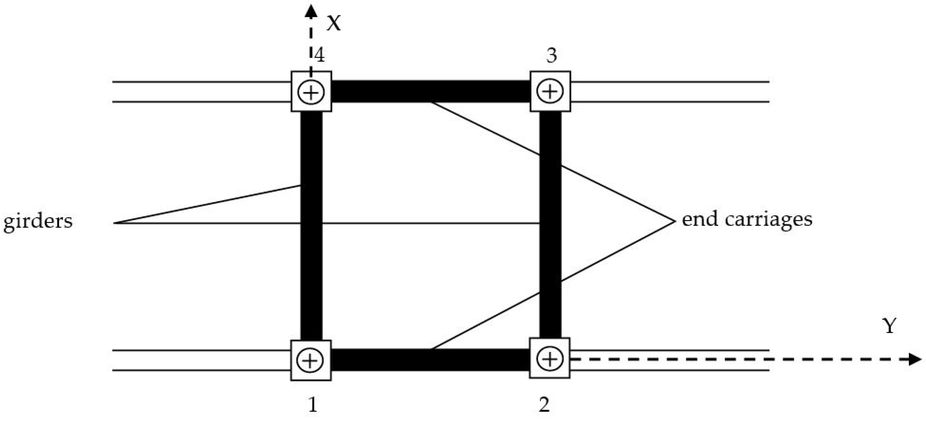
In order to provide proper work of the crane bridge, it is necessary to maintain perpendicularity of end carriages and girders, as well as parallel end carriages and girders (Figure 1). Most cases described in the available literature have not taken this issue into account while performing various types of specialized analyses [9,12,13].

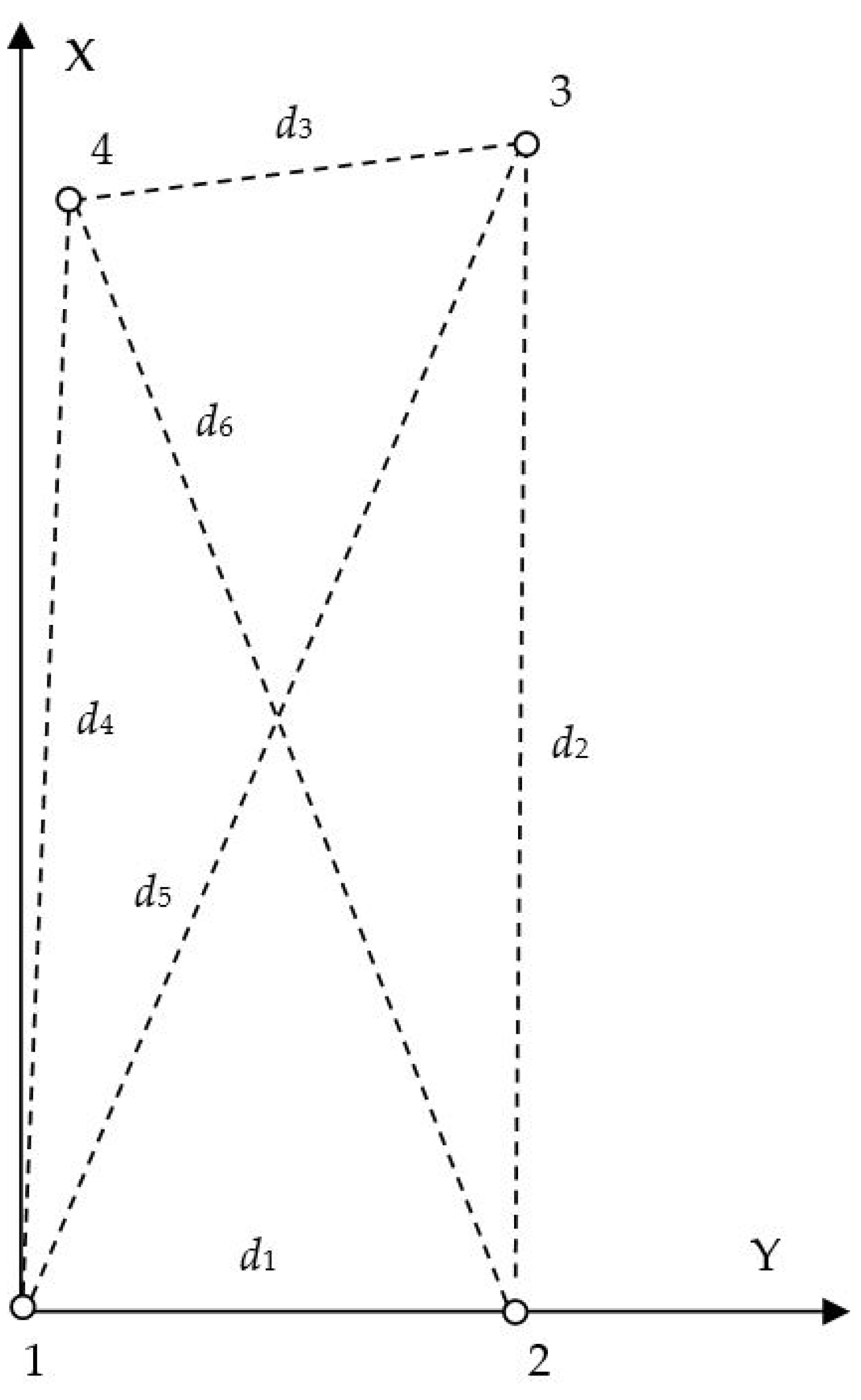
According to Figure 2, the following conditions of parallel character have been adopted:

$$\begin{array}{c}{\widehat{X}}_4-{\widehat{X}}_1-{\mathrm{d}}_4^t=0\\ {\widehat{X}}_3-{\widehat{X}}_2-{\mathrm{d}}_2^t=0\\ {\widehat{Y}}_2-{\widehat{Y}}_1-{\mathrm{d}}_1^t=0\\ {\widehat{Y}}_3-{\widehat{Y}}_4-{\mathrm{d}}_3^t=0\end{array}⇨\begin{array}{c}{X}_4^{ob}+d_{X_4}-X_1^{ob}-d_{X_1}-{\mathrm{d}}_4^t=0\\ X_3^{ob}+d_{X_3}-X_2^{ob}-d_{X_2}-{\mathrm{d}}_2^t=0\\ Y_2^{ob}+d_{Y_2}-Y_1^{ob}-d_{Y_1}-{\mathrm{d}}_1^t=0\\ Y_3^{ob}+d_{Y_3}-Y_4^{ob}-d_{Y_4}-{\mathrm{d}}_3^t=0\end{array}⇨\begin{array}{c}{d}_{X_4}-d_{X_1}+X_4^{ob}-X_1^{ob}-{\mathrm{d}}_4^t=0\\ d_{X_3}-d_{X_2}+X_3^{ob}-X_2^{ob}-{\mathrm{d}}_2^t=0\\ d_{Y_2}-d_{Y_1}+Y_2^{ob}-Y_1^{ob}-{\mathrm{d}}_1^t=0\\ d_{Y_3}-d_{Y_4}+Y_3^{ob}-Y_4^{ob}-{\mathrm{d}}_3^t=0\end{array}$$

(7)

where: ${\widehat{X}}_1,{\widehat{Y}}_1,{\widehat{X}}_2,{\widehat{Y}}_2,{\widehat{X}}_3,{\widehat{Y}}_3,{\widehat{X}}_4,{\widehat{Y}}_4$ are adjusted coordinates of controlled points located on the crane bridge.

The condition of perpendicularity between pairs of end carriages and girders should also be maintained, therefore:

$$\begin{array}{c}{\widehat{X}}_1-{\widehat{X}}_2=0\\ {\widehat{X}}_4-{\widehat{X}}_3=0\\ {\widehat{Y}}_4-{\widehat{Y}}_1=0\\ {\widehat{Y}}_3-{\widehat{Y}}_2=0\end{array}⇨\begin{array}{c}{X}_1^{ob}+d_{X_1}-X_2^{ob}-d_{X_2}=0\\ X_4^{ob}+d_{X_4}-X_3^{ob}-d_{X_3}=0\\ Y_4^{ob}+d_{Y_4}-Y_1^{ob}-d_{Y_1}=0\\ Y_3^{ob}+d_{Y_3}-Y_2^{ob}-d_{Y_2}=0\end{array}⇨\begin{array}{c}{d}_{X_1}-d_{X_2}+X_1^{ob}-X_2^{ob}=0\\ d_{X_4}-d_{X_3}+X_4^{ob}-X_3^{ob}=0\\ d_{Y_4}-d_{Y_1}+Y_4^{ob}-Y_1^{ob}=0\\ d_{Y_3}-d_{Y_2}+Y_3^{ob}-Y_2^{ob}=0\end{array}$$

(8)

For the conditions imposed on pseudo-observations, the height of controlled points can be presented in the form (all controlled points are located at the same height)

$$\widehat{Z}=0$$

(9)

2.2. Adjustment of Observations Results

The system of correction equations presented earlier as relation (5) can be written in the following matrix Form (10):

$$V=AX+\lambda$$

(10)

where:

• $V^T={[v_{{\mathrm{d}}_1},\dots ,v_{{\mathrm{d}}_n}]}^T$ is the vector of correction to pseudo-distances,
• $X^T={[d_{{\mathrm{X}}_1},d_{{\mathrm{Y}}_1},\dots ,d_{{\mathrm{X}}_m},d_{{\mathrm{Y}}_m}]}^T$ is the vector of increments to approximate parameters (coordinates of points),
• ${\lambda }^T={[{\mathrm{d}}_1^t-{\mathrm{d}}_1^{ob},\dots ,{\mathrm{d}}_i^t-{\mathrm{d}}_i^{ob}]}^T$ is the vector of deviations of theoretical lengths from the corresponding value of pseudo-observation (i is the number of pseudo-observations), and
• $A$ is the known matrix of coefficients standing at the estimated parameters of the model.

Applying the least squares method [14], specified in form of $V^{T}PV=\min$, the estimator of the parameter vector $\widehat{X}$ may be derived from the following equation:

$$\widehat{X}=-{\left(A^T{P}_{\mathrm{d}}A\right)}^{-1}{A}^T{P}_{\mathrm{d}}\lambda .$$

(11)

The matrix of weights assigned to the appropriate pseudo-observations is marked as $P_{\mathrm{d}}=Q_{\mathrm{d}}^{-1}$, whereas the matrix $Q_{\mathrm{d}}^{}$ is a matrix of pseudo-observation cofactors in the form of

$$Q_{\mathrm{d}}^{}=D{Q}_X{D}^T,$$

(12)

where the transformation matrix is

$$D=\left[\begin{array}{ccccc}\frac{\partial {\mathrm{d}}_1}{\partial X_1}& \frac{\partial {\mathrm{d}}_1}{\partial Y_1}& \cdots & \frac{\partial {\mathrm{d}}_1}{\partial X_m}& \frac{\partial {\mathrm{d}}_1}{\partial Y_m}\\ ⋮& ⋮& ⋮& ⋮& ⋮\\ ⋮& ⋮& ⋮& ⋮& ⋮\\ ⋮& ⋮& ⋮& ⋮& ⋮\\ \frac{\partial {\mathrm{d}}_n}{\partial X_1}& \frac{\partial {\mathrm{d}}_n}{\partial Y_1}& \cdots & \frac{\partial {\mathrm{d}}_n}{\partial X_m}& \frac{\partial {\mathrm{d}}_n}{\partial Y_m}\end{array}\right]$$

(13)

The matrix of cofactors:

$$Q_X=\left[\begin{array}{cccccc}{m}_{X_1}^2& \mathrm{c}\tilde{\mathrm{o}}\mathrm{v}(X_1,Y_1)& & & & \\ \mathrm{c}\tilde{\mathrm{o}}\mathrm{v}(X_1,Y_1)& m_{Y_1}^2& & & & \\ & & \ddots & & & \\ & & & \ddots & & \\ & & & & m_{X_m}^2& \mathrm{c}\tilde{\mathrm{o}}\mathrm{v}(X_m,Y_m)\\ & & & & \mathrm{c}\tilde{\mathrm{o}}\mathrm{v}(X_m,Y_m)& m_{Y_m}^2\end{array}\right]$$

(14)

was formed from the corresponding elements of the matrix $Q_{XY{Z}_j}$ designated earlier by the Form (3).

In order to assess the accuracy of the adjustment results obtained from Equation (11), the covariance matrix of the parameter vector $C_{\widehat{X}}$ is applied:

$$C_{\widehat{X}}=m_0^2{Q}_{\widehat{X}}$$

(15)

where $Q_{\widehat{X}}={\left(A^T{P}_{\mathrm{d}}A\right)}^{-1}$ is a matrix of cofactors and $m_0^2=\frac{{\widehat{V}}^T{P}_{\mathrm{d}}\widehat{V}}{n-r}$(n is the number of pseudo-observations, r is the number of parameters).

The accuracy analysis often employs the covariance matrix of corrections vector $C_{\widehat{V}}$:

$$C_{\widehat{V}}=m_0^2\left\{P_{\mathrm{d}}^{-1}-A(A^T{P}_{\mathrm{d}}A{)}^{-1}{A}^T\right\}$$

(16)

Equation (11) is obtained by means of the traditional least squares method and it is impossible to apply here the conditions imposed on the estimated parameters. In order to take into account conditions of parallel and perpendicular characters, and the imposed height of the controlled points (Equations (7), (8), and (9)), the adjustment task must be solved by the parametric method with the conditions on estimated parameters. This method has already been used and described by the authors in the works [1,2,3], and the broader theoretical considerations can be found in [15,16]. Only the main dependencies necessary to understand the presented solution will be presented below.

The parametric method with conditions corresponds to the following optimization task:

$$\begin{array}{l}AX+\lambda =V\\ BX+\Omega =0\\ V^T\tilde{P}V=\min \end{array}\}$$

(17)

The first dependence Equation (17), which corresponds to the traditional least squares method, has been explained above. The second equation, $BX+\Omega =0$, of Dependence (17) concerns the conditions imposed on the estimated parameters X. The elements of matrix B are the coefficients standing at the estimated parameters in Relations (7), (8), and (9). These coefficients may take the following values: −1, 0, and 1.

Vector $\Omega ={\left[\begin{array}{ccc}\underset{relation(7)}{\underbrace{X_4^{ob}-X_1^{ob}-{\mathrm{d}}_4^{\mathrm{t}},\dots }},& \underset{relation(8)}{\underbrace{X_1^{ob}-X_2^{ob},\dots }},& \underset{relation(9)}{\underbrace{0}}\end{array}\right]}^T$ is a vector of free terms in this equation.

In search of a solution to the optimization problem (17) by means of the least square method, the traditional method (e.g., [16]) or a simplified method involving the acceptance for free terms (occurring in the conditional equations) with enormously high values of weights [16] can be applied. The proposed solution method is based on the use of conditional equations, as additional equations of corrections, with very high values of weights, so that $V_{\Omega }=0$. Hence it reads as follows:

$$BX+\Omega =V_{\Omega }$$

(18)

The adoption of very high values of weights allows for the received correction values equal to zero within the limits of numerical calculations.

Taking these assumptions, the solution is simple enough to use the literature-bound parametric method [16]. Thus, the system of correction equations takes the form

$$\tilde{A}X+\tilde{\lambda }=\tilde{V}$$

(19)

where $\tilde{A}=\left[\begin{array}{l}A\\ B\end{array}\right]$, $\tilde{\lambda }=\left[\begin{array}{l}L\\ \Omega \end{array}\right]$, $\tilde{V}=\left[\begin{array}{l}V\\ V_{\Omega }\end{array}\right]$.

The adjustment criterion takes the following form:

$${\tilde{V}}^T\tilde{P}\tilde{V}=\min$$

where the weight matrix $\tilde{P}$ is $\tilde{P}=\left[\begin{array}{cc}{P}_{\mathrm{d}}& 0\\ 0& P_{\infty }\end{array}\right]$.

Hence,

$$\widehat{X}=-{({\tilde{A}}^T\tilde{P}\tilde{A})}^{-1}{\tilde{A}}^T\tilde{P}\tilde{\lambda }$$

(20)

Therefore,

$$\widehat{\tilde{V}}=-\tilde{A}{({\tilde{A}}^T\tilde{P}\tilde{A})}^{-1}{\tilde{A}}^T\tilde{P}\tilde{\lambda }+\tilde{\lambda }$$

(21)

In order to assess the accuracy of the obtained results, appropriate covariance matrixes are used as follows:

(1)

The covariance matrix $C_{\widehat{X}}$ of the parameter vector $\widehat{X}$,

$$C_{\widehat{X}}=m_0^2{Q}_{\widehat{X}}$$

(22)

where $Q_{\widehat{X}}={({\tilde{A}}^T\tilde{P}\tilde{A})}^{-1}$ is a matrix of cofactors.

(2)

The covariance matrix $C_{\widehat{\tilde{V}}}$ of the integrated corrections vector $\widehat{\tilde{V}}$,

$$C_{\widehat{\tilde{V}}}=m_0^2{Q}_{\widehat{\tilde{V}}}$$

(23)

where the covariance matrix $Q_{\widehat{\tilde{V}}}$ takes the form $Q_{\widehat{\tilde{V}}}=(\tilde{P}-\tilde{A}{\left({\tilde{A}}^T\tilde{P}\tilde{A}\right)}^{-1}{\tilde{A}}^T)$ and $m_0^2=\frac{{\widehat{\tilde{V}}}^T\tilde{P}\widehat{\tilde{V}}}{n-m}$(n is the number of pseudo-observations, m is the number of parameters).

3. Results

The theoretical considerations were verified on the basis of simulated data. Simulated data allow for the determination of the practical properties of the proposed method. Knowing the theoretical values, we can relate them to the results obtained from computations, and thus confirm or deny the proper work of the proposed method. The locations of controlled points (1, 2, 3, 4) on the crane bridge were adopted in accordance with Figure 1.

Theoretical values of the coordinates of the crane bridge’s controlled points are shown in

Table 1. List of theoretical coordinates of controlled points.

Point Number	${\mathit{X}}_{\mathit{i}}^{\mathit{t}}\left(\mathbf{mm}\right)$	${\mathit{Y}}_{\mathit{i}}^{\mathit{t}}\left(\mathbf{mm}\right)$	${\mathit{Z}}_{\mathit{i}}^{\mathit{t}}\left(\mathbf{mm}\right)$
1	0	0	0
2	0	3000	0
3	9000	3000	0
4	9000	0	0

.

Figure 2 presents the pseudo-distances adopted in the analyses. The values of individual theoretical distances ${\mathrm{d}}_k^t$ are included in

Table 2. Theoretical distances ${\mathrm{d}}_k^t$.

Distance Number	Distance Value ${\mathbf{d}}_{\mathit{k}}^{\mathit{t}}\left(\mathbf{mm}\right)$
$k=1$	3000
$k=2$	9000
$k=3$	3000
$k=4$	9000
$k=5$	9487
$k=6$	9487

.

Based on the simulated measurement results (horizontal angles, vertical angles, and distances) the following coordinates of the controlled points in the external coordinate system (coordinate system of the total station) were obtained (

Table 3. Coordinates of controlled points in the external coordinate system.

Point Number	${\mathit{X}}_{\mathit{i}}^{\prime }\left(\mathbf{m}\right)$	${\mathit{Y}}_{\mathit{i}}^{\prime }\left(\mathbf{m}\right)$	${\mathit{Z}}_{\mathit{i}}^{\prime }\left(\mathbf{m}\right)$
1	−4.500	−1.500	6.723
2	−4.500	1.503	6.717
3	4.508	1.506	6.715
4	4.499	−1.496	6.724

).

For the sake of the present inquiry, the local coordinate system (Figure 2) was adopted, whose origin is point 1 ($X_1=0,Y_1=0,Z_1=0$). It was assumed that the Y axis includes point 2 ($X_2^{\prime }=0$), hence $Y_2^{\prime }=3003$ mm (end carriage length determined on the basis of coordinates). The coordinates of controlled points on the object (

Table 4. Practical coordinates of points and their mean errors.

Point Number	${\mathit{X}}_{\mathit{i}}^{\mathit{o}\mathit{b}}\left(\mathbf{mm}\right)$	${\mathit{m}}_{{\mathit{X}}_{\mathit{i}}^{\mathit{o}\mathit{b}}}\left(\mathbf{mm}\right)$	${\mathit{Y}}_{\mathit{i}}^{\mathit{o}\mathit{b}}\left(\mathbf{mm}\right)$	${\mathit{m}}_{{\mathit{Y}}_{\mathit{i}}^{\mathit{o}\mathit{b}}}\left(\mathbf{mm}\right)$	${\mathit{Z}}_{\mathit{i}}^{\mathit{o}\mathit{b}}\left(\mathbf{mm}\right)$	${\mathit{m}}_{{\mathit{Z}}_{\mathit{i}}^{\mathit{o}\mathit{b}}}\left(\mathbf{mm}\right)$
1	0	0.6	0	0.9	0	2.2
2	0	0.6	3003	0.9	−6	2.2
3	9008	0.6	3004	0.9	−8	2.2
4	8999	0.6	2	0.9	1	2.2

) were obtained by means of transforming coordinates of the controlled points (Table 3).

The Relation (3) makes it possible to determine the values of mean errors of the coordinates of these points (Table 4).

The coordinates presented in Table 3 made it possible to determine the distance $d_k^{ob}$ between particular controlled points (

Table 5. Distances ${\mathrm{d}}_k^{ob}$ (pseudo-observations).

Distance Number	${\mathit{d}}_{\mathit{k}}^{\mathit{o}\mathit{b}}\left(\mathbf{mm}\right)$	${\mathit{m}}_{{\mathit{d}}_{\mathit{k}}^0}\left(\mathbf{mm}\right)$
$k=1$	3003	1.1
$k=2$	9008	1.1
$k=3$	3002	1.1
$k=4$	8999	1.1
$k=5$	9496	1.1
$k=6$	9486	1.1

) and the values of mean errors obtained from the Relation (12) ($m_{d_k^0}=\sqrt{{(Q_{\mathrm{d}})}_{ii}}$, ${(Q_{\mathrm{d}})}_{ii}$ is the diagonal element of the matrix). These distances will be further considered as pseudo-observations.

The computations were made due to the following three variants:

(1)

Variant 1: the least square method solution (Relation (11)).

(2)

Variant 2: solution according to the parametric method with the condition on heights (Relation (20)).

(3)

Variant 3: Variant 2 with conditions of perpendicularity and parallelism imposed on the estimated parameters (Relation (20)).

The coordinates of point 1 and the coordinate X of point 2 were assumed in the analysis.

The following computational results were obtained in the form of adjusted coordinates due to individual variants (

Table 6. Adjusted coordinates of controlled points of the crane bridge (in mm).

Adjusted Coordinates	Variant 1	Variant 2	Variant 3
${\widehat{X}}_3$	9008	9008	9000
${\widehat{X}}_4$	8999	8999	9000
${\widehat{Y}}_2$	3003	3003	3000
${\widehat{Y}}_3$	3005	3005	3000
${\widehat{Y}}_4$	3	3	0
${\widehat{Z}}_{j=1,2,3,4}$	−3	0	0

).

The correction values for the pseudo-observation $d_k^{ob}$ and the heights of particular controlled points calculated for all three variants are presented in

Table 7. Values of corrections for pseudo-observations (in mm).

Corrections	Variant 1	Variant 2	Variant 3
${\widehat{v}}_{d_1}$	0.0	0.0	−3.0
${\widehat{v}}_{d_2}$	−0.1	−0.1	−8.0
${\widehat{v}}_{d_3}$	0.0	0.0	−2.0
${\widehat{v}}_{d_4}$	−0.1	−0.1	1.0
${\widehat{v}}_{d_5}$	0.1	0.1	−9.0
${\widehat{v}}_{d_6}$	0.1	0.1	1.0
${\widehat{v}}_{Z_1}$	−3.3	0.0	0.0
${\widehat{v}}_{Z_2}$	2.8	6.0	6.0
${\widehat{v}}_{Z_3}$	4.8	8.0	8.0
${\widehat{v}}_{Z_4}$	−4.3	−1.0	−1.0
${\widehat{v}}_{Z^w}$	−	0.0	0.0

.

Table 8. Differences between object coordinates after the transformation step and adjusted coordinates (in mm).

	Variant 1	Variant 2	Variant 3
$\Delta {\widehat{X}}_1$	0	0	0
$\Delta {\widehat{X}}_2$	0	0	0
$\Delta {\widehat{X}}_3$	0	0	−8
$\Delta {\widehat{X}}_4$	0	0	1
$\Delta {\widehat{Y}}_1$	0	0	0
$\Delta {\widehat{Y}}_2$	0	0	−3
$\Delta {\widehat{Y}}_3$	1	1	−4
$\Delta {\widehat{Y}}_4$	1	1	−2
$\Delta {\widehat{Z}}_1$	−3	0	0
$\Delta {\widehat{Z}}_2$	3	6	6
$\Delta {\widehat{Z}}_3$	5	8	8
$\Delta {\widehat{Z}}_4$	−4	−1	−1

presents the differences between the adjusted coordinates of individual controlled points of the crane bridge and their coordinates obtained from the measurement.

The size of differences in values of the X and Y coordinates from Table 8 are shown schematically in Figure 3.

Referring to the results presented in Table 7, Table 8, and Figure 3, we note that differences in diagonal lengths allow for unambiguous interpretation of the obtained results, for example, whether these differences are acceptable or not in relation to existing national standards and technical guidelines. Comparing the theoretical values with the values obtained from the computations, we note that the most favorable results were obtained for Variant 3. Although the results obtained for this variant have the highest values, it should be noted that they include the conditions of perpendicularity and parallelism for end-carriages and girders as opposed to other variants, which affects the safe operation of the crane. Thus, for example, the obtained difference in Variant 3 for the diagonal length $d_5$, which is −9 mm, should be in accordance to existing standards in the range $\langle -5 \mathrm{mm};5 \mathrm{mm}\rangle$, so the value obtained from the computations is significant. The use of statistical tests (significance), for example, $k{m}_d<v_{d_i}$ (where $m_d$ is the value of the mean error determined for the diagonal) may lead to erroneous interpretation of the results. This happens due to the adopted values of the parameter k whose value is not strictly determined and depends on knowledge and engineering experience of the measurement contractors.

4. Discussion

The authors proposed a new method of checking the geometrical conditions of crane bridges. Their detailed theoretical and empirical analysis assumed that the measurement results, subject to further elaboration, were obtained by means of a total station. Numerical computations were made in three different variants taking into account the traditional least square method, a parametric solution with the conditions on the heights of the points and a parametric solution with the conditions on heights and conditions of parallel and perpendicular characters imposed on the parameters. The first two solutions lead to the same results for parameters and distances, whereas considering the adopted condition in the second variant, the obtained results for heights were different. The results of the third solution were different from the former variants. The difference originates from the adopted conditions of parallelism and perpendicularity, and according to the authors these should be met to ensure safe and efficient work of the crane. The proposed solution indicates that both second and third computational variants can be employed to check the geometrical conditions of the crane bridge, however, the third variant additionally takes into account the relations that occur between the girders and end carriages, which is crucial from the authors’ viewpoint. Therefore, the authors recommend using the third variant of computations to solve the problem presented in the article. Although the computations were performed on simulated data, it is assumed that the presented analysis may also be valid for real data. In their further studies, the authors will focus on checking and using modern instruments, and verifying which geometrical conditions must be met by crane wheels to prevent failures in crane operation. That research will help to create a comprehensive measurement technology with calculations using modern statistical methods and interpret of the obtained results. Due to the fact that displacements are often caused by locations of objects on unfavorable geotechnical conditions, the issue presented in the paper constitutes an important problem in reference to geosciences. The proposal presented in this paper can also be used (after some modification) in tests of other steel constructions, for example, in tests of roof displacements of industrial halls, warehouses, sports stadiums, etc.

Most important subscripts and variables used in the paper:

• $X_j^{\prime },Y_j^{\prime },Z_j^{\prime }$ coordinates in local coordinate system of the instrument (external coordinate system)
• X, Y, Z coordinates in local coordinate system of the crane bridge (internal coordinate system)
• $Q$ matrix of cofactors
• $P$ weight matrix
• $C$ covariance matrix
• $D$ transformation matrix
• $A,B$ known matrix of coefficients
• $V$ vector of corrections
• $X$ vector of parameters
• $m_X,m_Y,m_Z$ mean errors of coordinates in the external coordinate system.