Comparison of Earthquake-Triggered Landslide Inventories: A Case Study of the 2015 Gorkha Earthquake, Nepal

Abstract

Despite landslide inventories being compiled throughout the world every year at different scales, limited efforts have been made to critically compare them using various techniques or by different investigators. Event-based landslide inventories indicate the location, distribution, and detected boundaries of landslides caused by a single event, such as an earthquake or a rainstorm. Event-based landslide inventories are essential for landslide susceptibility mapping, hazard modeling, and further management of risk mitigation. In Nepal, there were several attempts to map landslides in detail after the Gorkha earthquake. Particularly after the main event on 25 April 2015, researchers around the world mapped the landslides induced by this earthquake. In this research, we compared four of these published inventories qualitatively and quantitatively using different techniques. Two principal methodologies, namely the cartographical degree of matching and frequency area distribution (FAD), were optimized and applied to evaluate inventory maps. We also showed the impact of using satellite imagery with different spatial resolutions on the landslide inventory generation by analyzing matches and mismatches between the inventories. The results of our work give an overview of the impact of methodology selection and outline the limitations and advantages of different remote sensing and mapping techniques for landslide inventorying.

1. Introduction

Landslides are the most frequent hazards of mountain regions throughout the world [1]. Given landslides’ variable characteristics, they cause enormous damage to human life and infrastructure [2]. Landslides are usually caused by a trigger, like an earthquake or rainfall, and these two phenomena are considered to be the common physical triggers for event-based landslides [3]. In the Himalayan region, rainfall in the monsoon period triggers several massive and small landslides every year [4]. However, landslides triggered by earthquakes are severely destructive. For instance, the recent global landslide triggering events of the Wenchuan earthquake (2008), China [5], the Gorkha earthquake (2015), Nepal [6], and the Bihar earthquake (2002), India [7], resulted in a large number of casualties and severe damage to private and public infrastructures. However, there are several reasons that make it difficult to extract information about the exact location of landslides in an area, such as difficulty in accessing the hazard-affected remote areas [1]. A landslide inventory map, including the exact location and the exact boundaries along with the distribution, is the prerequisite for landslide analysis, susceptibility assessment, and mapping [8,9]. Furthermore, for the case of event-based landslides, detailed and state-of-the-art information about the landslides is critical. To better understand the triggering factors in an event-based landslide, different aspects of tracking, recording, and analysing data must be considered [10]. Several definitions are available regarding landslide inventories in the literature. According to [11], landslide inventory maps are the basis for obtaining records about the date of occurrence, location, and type of slope movements. A dataset of a landslide inventory can provide information on the time of the event, the location of occurrence, the type of landslide, and the extent of the landslide [12].

Landslide inventory maps are the basis of determining hazard and risk assessment [13,14]. Golovko et al. [15] analyzed multiple sources of slope failures for the establishment of a comprehensive multitemporal landslide inventory. They also described landslide inventories as the prerequisite to enable landslide hazard assessment. Landslide inventories are also crucial in carrying out a risk analysis by analyzing the impacts of past landslide events and relating them to the present criteria to predict future landslide-prone areas [16]. Thus, it is crucial to record required information on landslide occurrence to link this with triggering factors.

Landslide inventory maps can give information about probable threatened areas to disaster management authorities whcih can be used for reconstruction planning after an earthquake event [6]. Inventories are also a basis for training and validating various knowledge-based, machine learning, and deep learning methodologies related to automatic landslide detection [1,14].

Event-based landslide inventory maps can be prepared from various sources. Recently, the availability and use of high-resolution remote sensing optical images has been very useful in the identification of landslides [14]. For instance, triggering events like earthquakes trigger thousands of landslides in remote areas. Therefore, remote sensing and earth observation (EO) data play a significant role in mapping and analyzing inventories. The EO data of pre- and post-landslide events are required for conducting classification and interpretation of the hazard-affected area. There have been several attempts to map landslides using expert-based approaches, such as manual rule-based, automatic, and semi-automatic classification techniques. Two main approaches for the classification and extraction of landslides from the EO data, namely object-based and pixel-based, were distinguished [1]. However, the spatial resolution of the available EO data plays a critical role in the quality of the resulting landslide inventory maps [17,18]. Although most studies so far relied on EO data with a single scale for landslide extraction, some works considered multi-resolution satellite imageries and EO data [18]. Even using a single satellite image frame, some studies performed multi-scale methodologies and observed higher landslide extraction accuracies compared to single-scale performances [17]. Scientific progress toward pixel-based automatic identification of landslides was made using remote sensing imageries with different resolutions [19]. Considerable progress toward pixel-based automatic identification of landslides was achieved using deep-learning convolution neural networks (CNN) [1,14]. Ghorbanzadeh et al. [1] applied CNN and other machine learning models to identify landslides in RapidEye data from the Rasuwa district in Nepal. The extracted landslides from different models were then tested using Global Position System (GPS) data along with a manually detected landslide inventory of image spectral features from RapidEye data; topographic input was also used, including digital elevation models (DEM) from Advanced Land Observing Satellite (ALOS) data. In another pixel-based study [20], unsupervised classification resulted in the detection of about 60% of manually extracted and mapped landslides. There were also several object-based studies for landslide extraction, such as [21] and [22], which compared their results with manually extracted results. Therefore, manual landslide extraction and mapping is considered a standard technique for receiving the most detailed and accurate inventory. As manual detection and extraction is the most reliable technique for inventory generation, it is preferable for testing state-of-the-art models, such as deep-learning CNN models. Therefore, the quality of the manually detected landslide inventory is critical, as it usually considered to be the ground truth [14]. There are a limited number of landslide and mass movement detection studies evaluating the quality of their applied inventory dataset. In a specific study [14], the frequency area distribution (FAD) method was applied to evaluate the three available landslide inventory maps, with one of them being selected for validation of the results.

On one hand, the quality of a landslide inventory map easily affects the overall accuracy of any landslide detection, susceptibility assessment, or hazard- and risk- mapping study. On the other hand, there are a limited number of landslide studies that tackled the problem of comparison of two or more inventories [3,23]. Pellicani and Spilotro [23] compared archives and surveyed inventories for the Daunia region in Italy. They compared two landslide inventory maps to determine the corresponding quality through direct comparison. Another work by [3] compared photo-interpreted and semi-automatic landslide inventory maps in the Pogliaschina catchment, Italy. They compared the quality of rainfall event-based inventories cartographically and statistically.

Quality and completeness levels of a landslide inventory depend upon the accuracy, certainty, and type of information included in the map [24]. Criteria for the assessment of inventories are lacking from previous landslide research [3,25,26]. For the comparison of inventories, two or more inventories are needed to compare the quality of landslide maps. Despite the great importance of establishing the quality of a landslide inventory for scientific investigations, the number of such studies is limited. Comparing two or more inventories does not occurs often due to the limited availability of two or more inventories. However, there are some studies that were carried out regarding landslide mapping, and also several databases of landslides were compiled earlier by [27,28]. After the 1989 Loma Prieta, California, earthquake (Mw 6.9) a total of 1046 landslides were mapped using field investigations and aerial photographs in an area of about 15,000 km² in central California. The spatial distribution of the landslides was investigated statistically using one-way analysis of variance (ANOVA) and regression techniques. Correlations of landslide occurrence with distance from the earthquake source, slope steepness, and rock type were determined [29]. A comprehensive database of devastating landslides caused by catastrophic earthquakes that took place all over the world was compiled by Rodríguez et al. [28], covering the period 1980–1997. Another work by Esposito et al. [30] discussed and described the ground effects and landslides triggered by the 1997 Umbria–Marche seismic sequence in an area of 700 km². The environmental, seismic intensity (ESI) scale, and earthquake hazard were studied by [31,32]. The ESI scale is a measurement which defines the earthquake intensity by considering the size and spatial distribution of earthquake environmental effects. Lekkas et al. [33] used the ESI scale and its correlation with geological structures for seismic hazard estimation of the 2008 Mw 7.9 Wenchuan, China, earthquake. In another study by [34], correlations between ESI-07 intensity, slope, and lithology were discussed regarding landslides triggered by the 2016 Mw 7.8 Pedernales, Ecuador, earthquake.

Furthermore, Ferrario et al. [35] investigated the role of earthquake environmental effects within seismic sequences from the 2018 Lombok (Indonesia). Statistical analysis was carried out for three nearly complete landslide inventories triggered by the 12 May 2008, Wenchuan Mw 7.9 earthquake of China [36]. Correlations of landslide occurrence with topographical factors and seismic parameters were studied for three inventories. This literature review shows that, over the past decades, there was an improving trend regarding both the documentation and statistical evaluation of the earthquake-induced landslides in some important works.

Several of the nowadays commonly applied methodologies were mostly developed by the Italian groups for the census of the effects induced by earthquakes of moderate magnitude. During the Emilia Romagna (northern Italy) 2012 earthquake sequence, for processing and real-time data sourcing, new approaches and technologies were developed by the INGV EMERGEO working group [37]. Just after the earthquake event, the EMERGEO working group surveyed the epicentral area for co-seismic geological hazards. Later, they organized the records and processed them with the EMERGEO Information System (siE). The EMERGEO working team of Civico et al. [38] presented a 1:25,000 scale map of the surface ruptures after the 30 October 2016 Mw 6.5 Norcia earthquake, central Italy. They used 11,000 oblique photographs taken from helicopter flights, which were verified with field datasets. They also provided the datasets through a database of the co-seismic effects following the Norcia earthquake [39].

In this study, we evaluated four manually extracted landslide inventory maps of the Gorkha earthquake 2015, Nepal. Four different research teams from different parts of the world carried out landslide inventories related to this earthquake and published their resulting maps. These studies used various EO data sources, such as very high-resolution WorldView imagery and coarser-resolution imageries. We compared these inventory maps quantitatively and qualitatively using the cartographical degree of matching and frequency area distribution (FAD) methods [40]. The reasons for the differences are discussed here, outlining the limitations and advantages of different mapping techniques.

2. Study Area

The epicentre of the earthquake was in the Gorkha district and its aftershock was about 140 km in the Dholaka district [41]. However, landslides triggered by the earthquake and several aftershocks were scattered around large areas. Seven districts that were severely affected by the earthquake were selected for inventory mapping by different researchers. The study area covered a 14,502 km² region, which spread over most of central Nepal. The area had two primary drainage systems, namely Narayani and Saptakoshi [42]. Our case study area lay in central Nepal country within the fold and thrust zone of Himalaya. This zone was caused by the collision of the Eurasian plate with the Indian Plate [43] (see Figure 1). The collision resulted in extensive crustal shortening and upheaval, leading to the formation of the quintessential collided orogen, Himalaya. All evaluations of the present study were done based on an overlapping region of four considered inventory maps.

3. Landslide Inventory Maps of Gorkha Earthquake (National Scale)

3.1. Inventory A

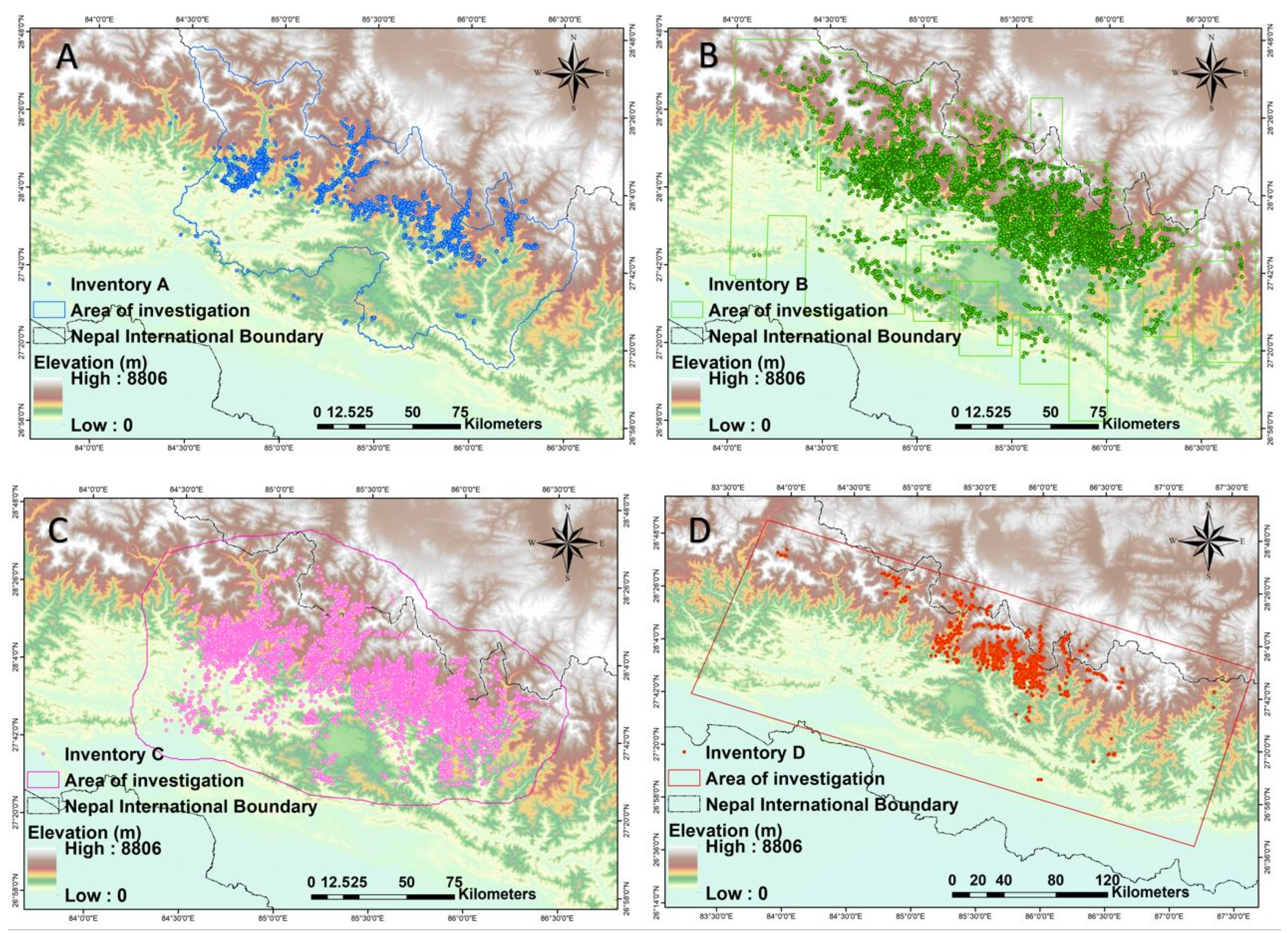
Authors carried out a field survey and manual interpretation of Landsat-8 Enhanced Thematic Mapper (ETM) images with a resolution of 15 m, Gaofen-1 (GF-1) images with resolution of 2 m, GF-2 images with resolution of 0.8 m, and Google Earth imagery to prepare the polygon-based inventory [42]. A total of 15,456 km² area was selected for investigation based on previous studies and updates during the digitation process. A total of 3716 co-seismic landslides were mapped. The largest landslide mapped was 9983 m² and the smallest landslide was less than 50 m². The co-seismic landslides covered a total area of 15.93 km².

3.2. Inventory B

Earthquake-induced landslides were mapped by comparing pre- and post-event very high-resolution satellite imageries. DigitalGlobe WorldView-2 and -3 imagery, along with Pleiades satellite data, were used [44]. The spatial resolution of imagery used in mapping landslides varied from 30–50 cm in most of the areas. Images were acquired from 26 April to 15 June 2015, with most images collected between 2 May and 8 May 2015. This team was the only group working on Gorkha earthquake who differentiated between landslide source and deposits areas. They were able to map more than 25,000 landslides in the area affected by the earthquake.

3.3. Inventory C

Authors used Google Earth imagery, which was updated after the Gorkha earthquake, to prepare a polygon-based inventory. A total of 4000 km² area was selected for investigation based on previous studies and updates during the digitizing process [45]. In most of the region, the satellite imagery of pre-earthquake was from December 2014 and post-earthquake imagery from 2–4 May, which was around one week after the main earthquake. A total of 17,000 co-seismic landslides were mapped by [45]. Results also showed the spatial correlation of topographical parameters with landslide occurrence.

3.4. Inventory D

The landslide inventory map was manually mapped by the authors in the immediate aftermath of the earthquake using a range of EO data sources, including web-hosted high-resolution optical data in Google™ Crisis Response (e.g., United Kingdom - Disaster Monitoring Constellation-2 (UK-DMC2), Disaster Monitoring Constellation for the International Charter (DMCii), Worldview, Digital Globe Inc., SPOT National Centre for Space Studies (CNES), imagery accessed via the Disaster Charter, imagery available from United States Geological Survey (USGS) Hazards Data Distribution System (HDDS Explorer), and imagery specifically tasked over regions of interest (e.g., Pleiades CNES). A total of 2117 co-seismic landslides were mapped by [46] (see Figure 2).

4. Landslide Inventory Comparison Methodologies

4.1. Spatial Distribution

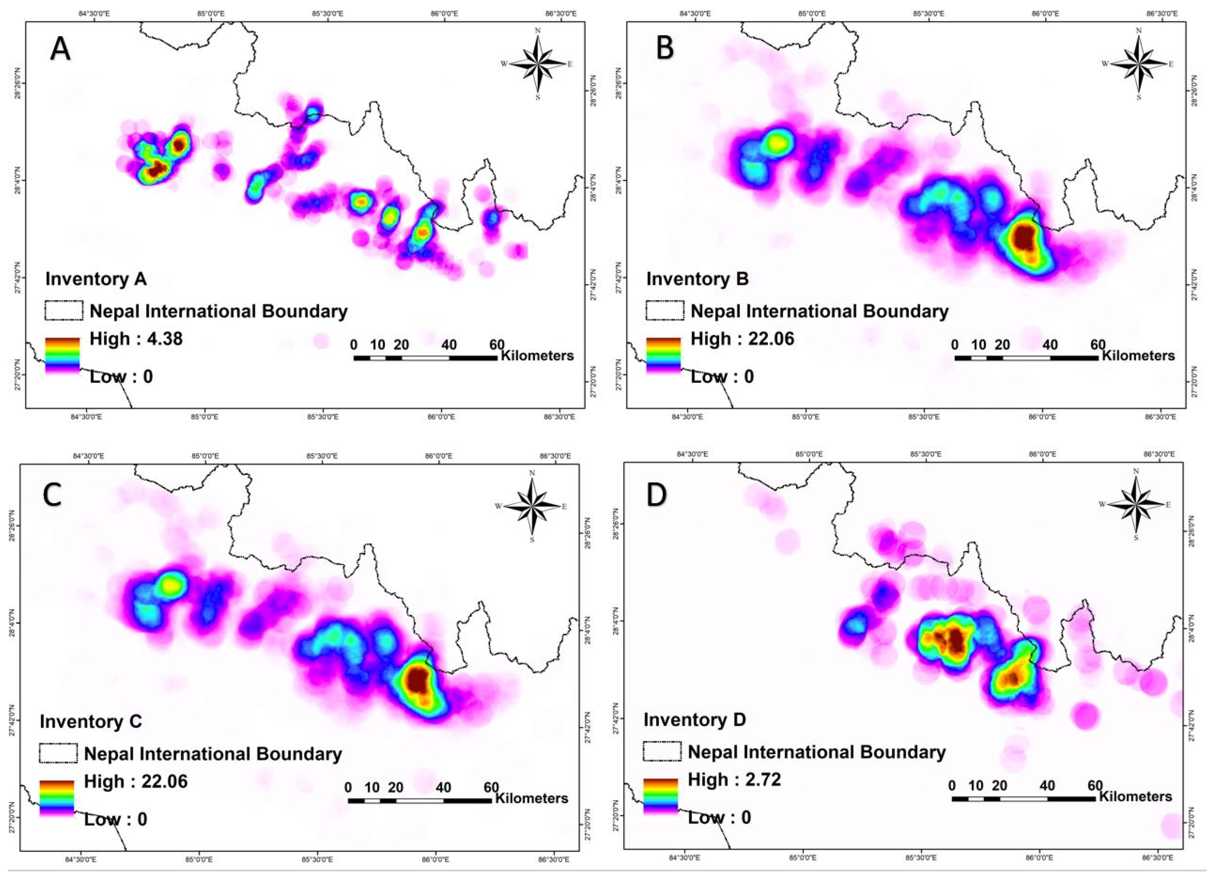
Landslide inventories for the Gorkha event were collected from various sources. Detailed information on inventories is given in

Table 1. Landslide inventories prepared after the 2015 Gorkha earthquake, Nepal.

#	Landslide Inventory	$\mathbf{No}.\mathbf{of}\mathbf{Landslides}\left({\mathit{N}}_{\mathit{L}\mathit{T}}\right)$	Geometry Type	Area Coverage	Produced by
1.	Valagussa et al. (2016)	4300	Polygon	Central Nepal	[48]
2.	Roback et al. (2018)	24,915	Polygon	Central Nepal	[44]
3.	Martha et al. (2017)	15,551	Polygon	Central Nepal	[49]
4.	Regmi et al. (2016)	2645	Polygon	Central Nepal	[42]
5.	Meena, Mavrouli, and Westen (2018)	2513	Polygon	Central Nepal	[50]
6.	Kargel et al. (2016)	4312	Polygon	Central Nepal	[51]
7.	Gnyawali et al. (2016)	19,332	Point	Central Nepal	[45]
8.	Robinson et al. (2017)	2117	Polygon	Central Nepal	[46]

. Out of the inventories, we used four that were available and prepared by research teams from various parts of the world. To analyze the landslide density per square kilometre, point-based inventory data were used. Figure 3 shows the landslide density distribution of selected inventories for the Gorkha event; all of the inventories were co-seismic and prepared using post-earthquake satellite imageries.

Information regarding the data used to prepare the inventories is given in Table 1. There was a significant variation in the number of landslides mapped for the Gorkha event, ranging from $N_{LT}=2117\mathrm{to}{N}_{LT}=24,915$. None of these inventories classified the types of landslides as proposed by [47]. The data sources used for mapping varied from high-resolution imagery of about 30 cm resolution to Google Earth images. The landslide density analysis results, illustrated in Figure 3, showed that most of the landslides were concentrated in the Gorkha and Sindhupalchock districts for most of the inventories; the southern part of the Rasuwa district was also severely hit, as can be interpreted from the Figure 3. Differences in the density of landslides in an area depended on factors such as the effect of amalgamation while mapping, the purpose of the mapping, and the data sources used for mapping. Areas near the Dholaka and Sindhupalchok districts showed high landslide density ias a result of the aftershock on 12 May 2015 in the Dholaka district. The higher density of landslides showed that inventories were prepared after the aftershock of 12 May 2015 and hence had a larger number of landslides compared to inventories prepared for the first earthquake event. Another factor that affected the density of landslides was the different coverage of the mapping area. Comparing the different inventories at larger scale is not an easy task as their coverage areas are different. To compare landslide inventories prepared by different interpreter, we chose a commonly mapped area that was mapped by most of the inventories. For the analysis, we chose four inventories from various sources which were polygon-based, and compared them statistically for smaller regions.

To compare the inventories for the Gorkha earthquake, we chose four polygon-based inventories that were available. The commonly mapped area was covered in all four inventories, which allowed for the statistical comparison of the inventories. We compared the four inventories and examined the differences and similarities of the total area covered, the number of landslides mapped, and the size of the landslides.

4.2. Cartographical Degree of Matching

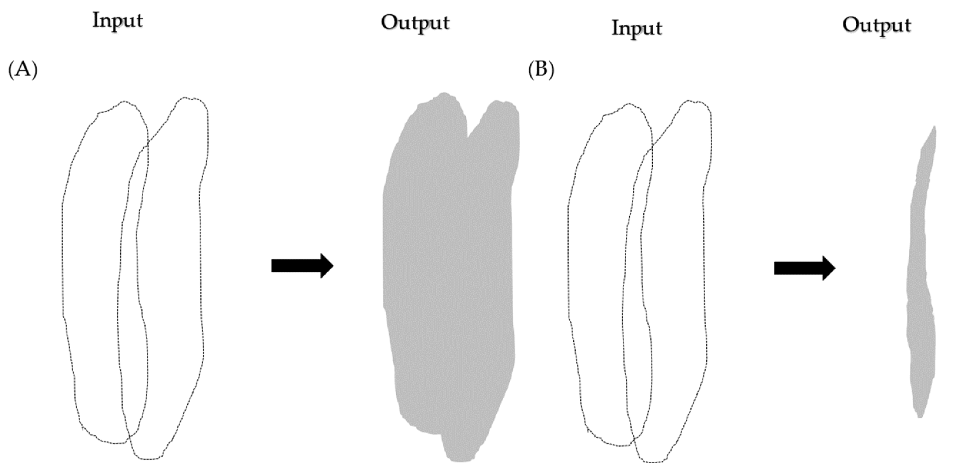
For the comparison of four inventories available for the common mapped area in the Rasuwa district, an attempt was made to determine the cartographic matching and mismatch (see Figure 4).

Carrara et al. (1993) [52] provided a method to evaluate the degree of matching and mismatch between two inventory maps. The mismatch index, $E$, was given by

$$E=\frac{\left(A_1{\displaystyle \cup }{A}_2\right)-\left(A_1{\displaystyle \cap }{A}_2\right)}{\left(A_1{\displaystyle \cup }{A}_2\right)},0\le E\le 1$$

(1)

$$M=1-E,0\le M\le 1$$

(2)

where E is the mismatch and M is the matching between the inventories. Union and intersection are used in Equation (1) to observe the matching and mismatch between the inventories.

This equation was valid for up to two inventories. However, in our case, we wanted to compare four inventories. Thus, we formulated an equation for the comparison of four inventories (see Equation (3)).

$$E=1-\frac{\left(A{\displaystyle \cap }B\right){\displaystyle \cup }\left(A{\displaystyle \cap }C\right){\displaystyle \cup }\left(A{\displaystyle \cap }D\right){\displaystyle \cup }\left(B{\displaystyle \cap }C\right){\displaystyle \cup }\left(B{\displaystyle \cap }D\right){\displaystyle \cup }\left(C{\displaystyle \cap }D\right)}{\left(A{\displaystyle \cup }B{\displaystyle \cup }C{\displaystyle \cup }D\right)}$$

(3)

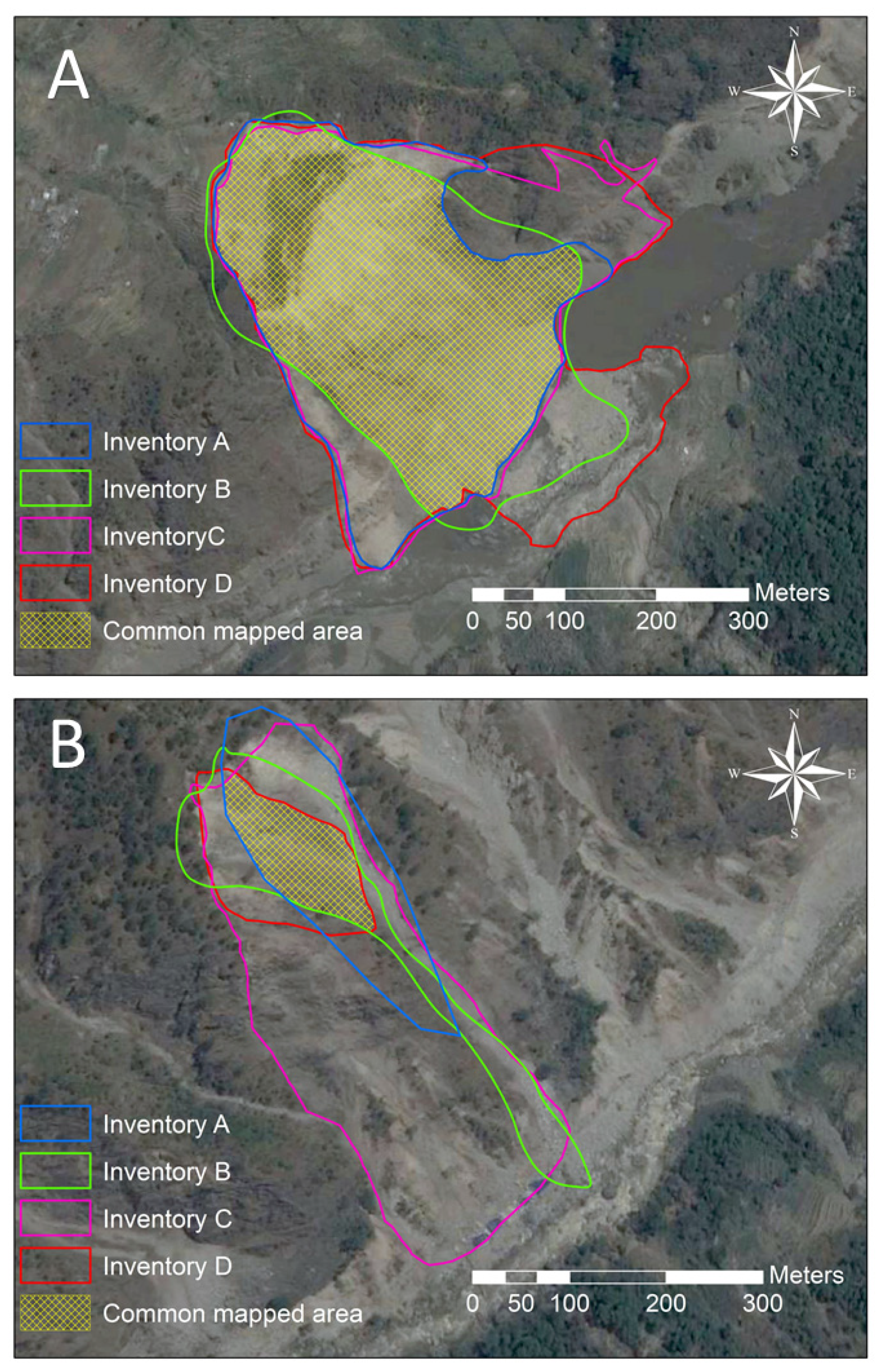
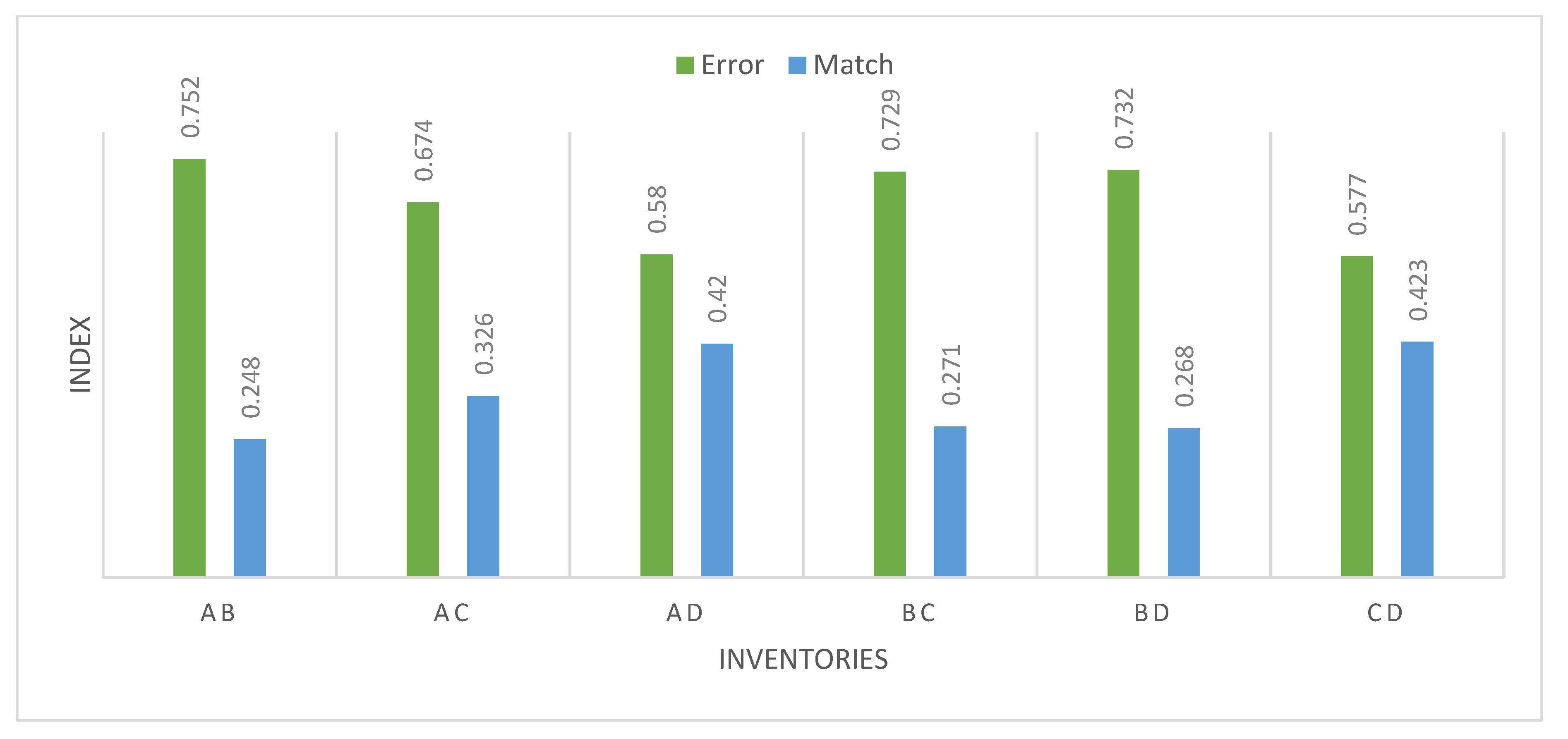
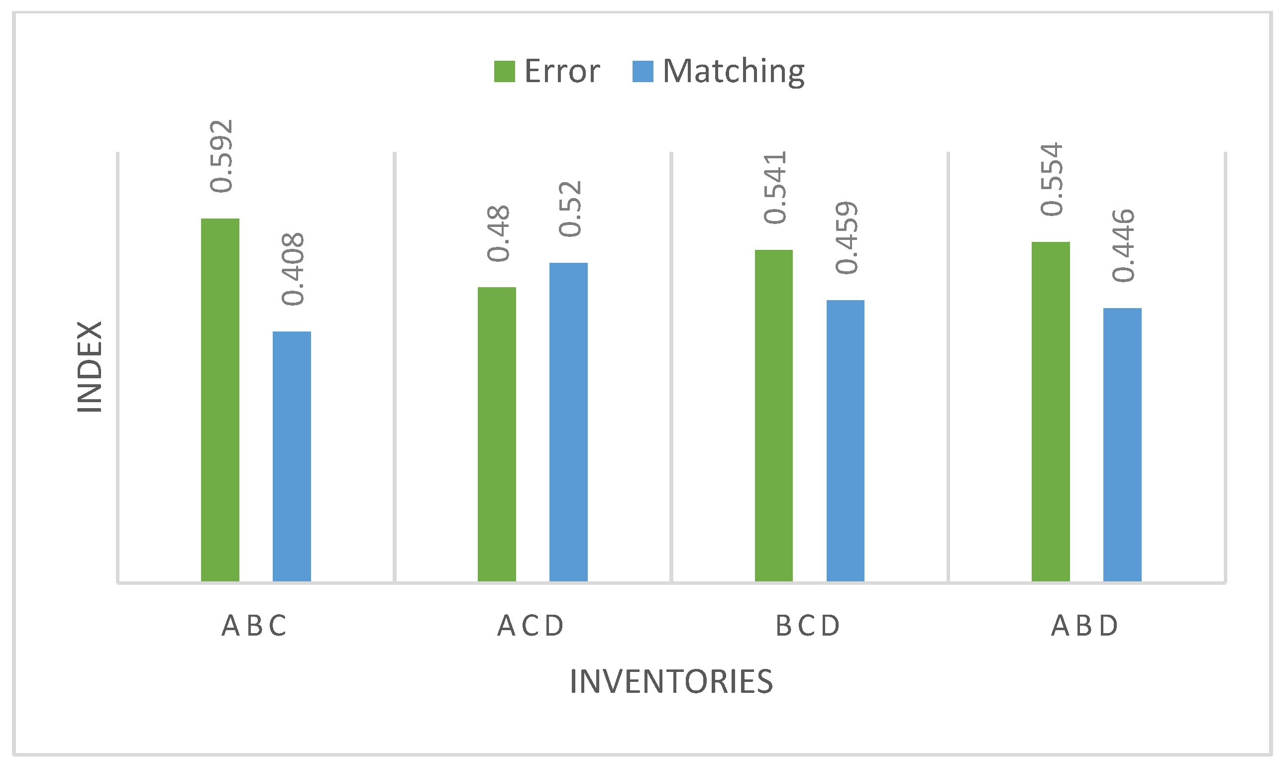
The statistics of the four landslide inventories can be seen in

Table 2. Statistics for the four event-based landslide inventories.

	A	B	C	D
Number of mapped landslides #	144	498	197	336
Minimum landslide area (m²)	500.53	35.50	95.49	112.22
Maximum landslide area (m²)	157,265.25	118,805.11	764,038	151,708.90
Mean landslide area (m²)	9990.18	6520.23	25,599.34	8816.13
Standard deviation of landslide area (m²)	19,203.38	11,595.57	74,255.39	17,832.65
Total landslide area (m²)	1,438,587.08	3,247,077.22	5,043,071.10	2,962,222.12

. The total number of landslides varied from 33 to 49 for the same area. Moreover, there was a significant difference in the total area of landslides. Cartographical mapping differences in a single landslide for the same event can be seen in Figure 5. Interpreters mapped the landslide boundary differently, and the causes of such differences are discussed in Section 5. Based on Equation (3), we observed cartographical match and mapping errors, as presented in

Table 3. Cartographical matching and mismatch between inventories.

Inventories	Area m²	Percentage of the Area Covered Relative to the Total Study Area	Mapping Error, E	Mapping Match, M
Landslide area Inventory A	294,0746.32	6.49
Landslide area Inventory B	3,256,245.33	7.18
Inventory A ∪ Inventory B	4,966,842.26	10.96
Inventory A ∩ Inventory B	1,231,685.97	2.72	0.752	0.248
Landslide area Inventory A	2,940,746.32	6.49
Landslide area Inventory C	5,043,072.67	11.12
Inventory A ∪ Inventory C	6,005,657.34	13.25
Inventory A ∩ Inventory C	1,960,725.08	4.32	0.674	0.326
Landslide area Inventory A	2,940,746.32	6.49
Landslide area Inventory D	4,230,476.82	9.33
Inventory A ∪ Inventory D	5,051,960.15	11.14
Inventory A ∩ Inventory D	2,122,932.49	4.68	0.58	0.42
Landslide area Inventory B	3,256,245.33	7.18
Landslide area Inventory C	5,043,072.67	11.12
Inventory B ∪ Inventory C	6,518,452.96	14.38
Inventory B ∩ Inventory C	1,765,857.66	3.90	0.729	0.271
Landslide area Inventory B	3,256,245.33	7.18
Landslide area Inventory D	4,230,476.82	9.33
Inventory B ∪ Inventory D	5,909,070.8	13.03
Inventory B ∩ Inventory D	1,582,813.94	3.49	0.732	0.268
Landslide area Inventory C	5,043,072.67	11.12
Landslide area Inventory D	4,230,476.82	9.33
Inventory C ∪ Inventory D	6,530,387	14.40
Inventory C ∩ Inventory D	2,764,641.79	6.10	0.577	0.423

. The pairwise comparison of inventories and comparison of inventories mapped by different interpreters are represented in Figure 6 and Figure 7, respectively.

4.3. Frequency Area Distribution (FAD)

Landslide inventories were statistically analyzed using frequency area distribution (FAD) curves, in which the landslide areas were plotted versus the cumulative and non-cumulative landslide frequencies. In the study by [53], observations showed that the power law was valid for medium and large landslides. The probability of occurrence of landslide size can be given by the power-law equation.

$$p\left(x\right)=c{X}^{-\beta },$$

(4)

where X is the observed values, c is a normalization constant, and β is the power-law exponent.

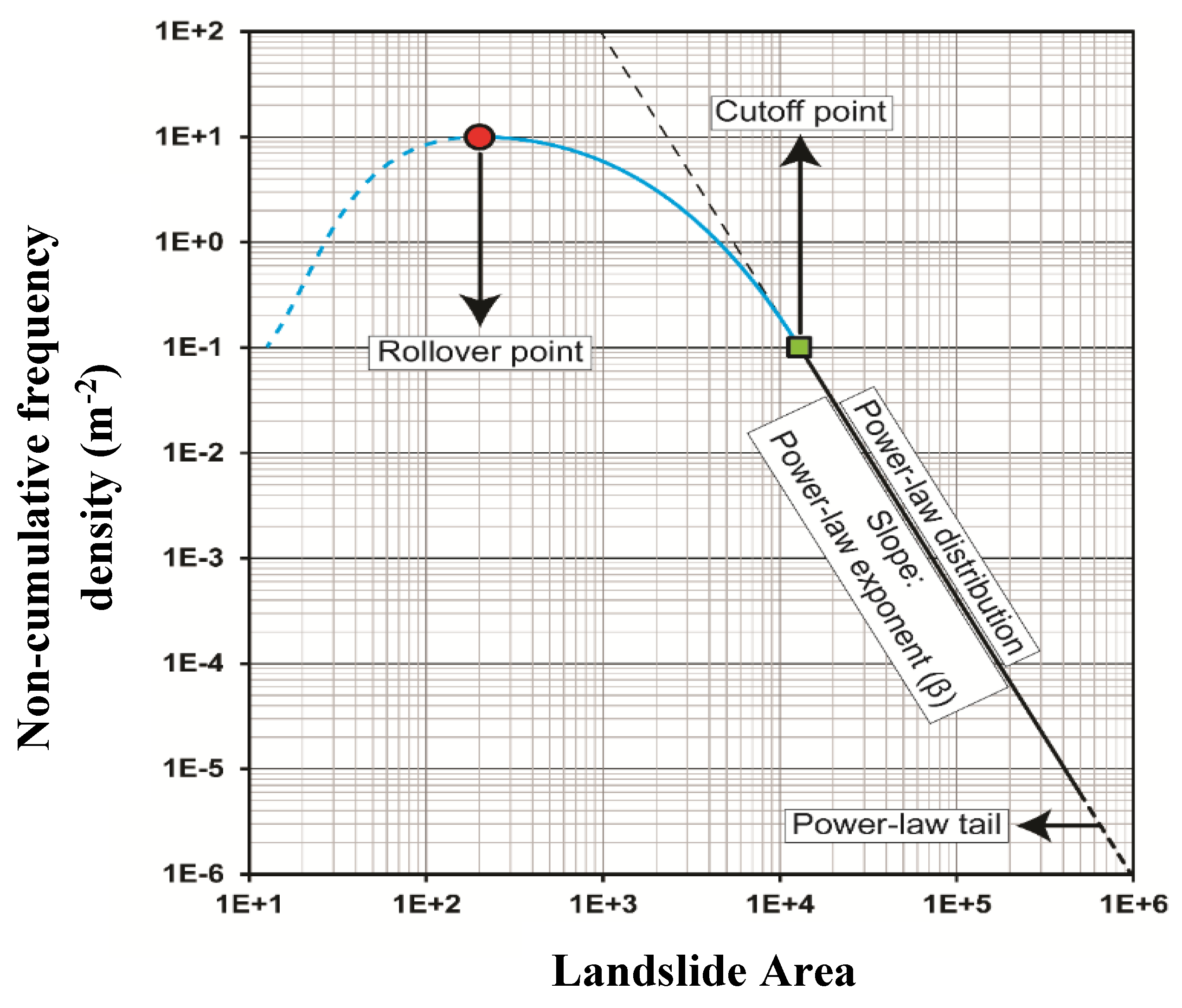
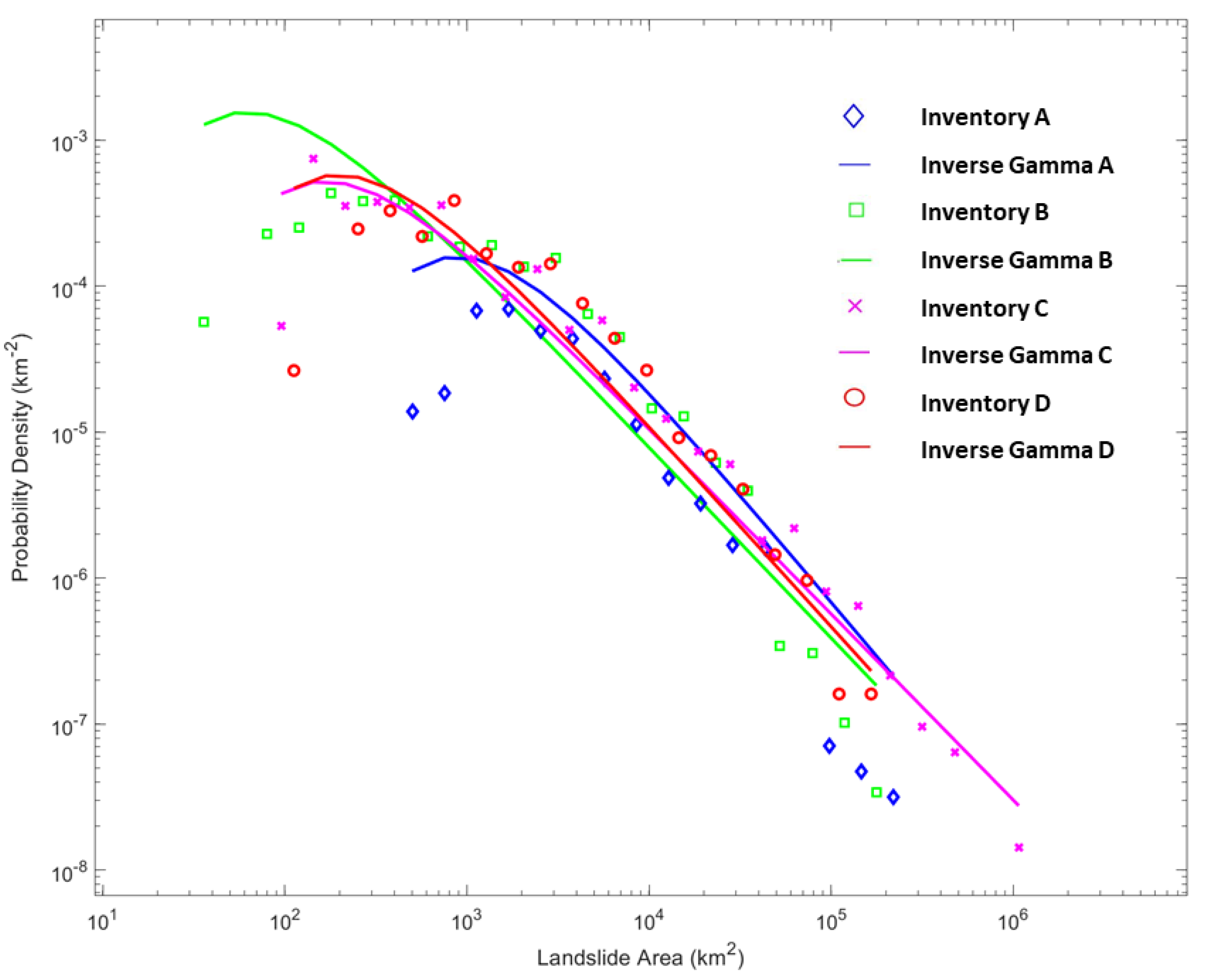
Figure 8 shows the power-law distribution for medium to massive landslides and divergence from the power-law toward lower frequencies with a rollover point, where frequency decreased for smaller landslides. The trend of the FAD of most landslide inventories diverged from the power-law for small landslides [53,54,55,56]. The point where this divergence began was defined as the cut-off point [56,57]. For non-cumulative probability density distributions of landslide areas, the peak point of the probability distribution curve, after which the probability value began to decrease for smaller landslides following a positive power-law decay, was referred to as the rollover point [58]. According to [58], in a power-law distribution, the slope of the distribution was defined with a power-law exponent. The part that was represented by large events was referred to as the power-law tail, as shown in Figure 9 (with a scaling parameter, β). Malamud et al. [53] investigated four well-documented landslide events and concluded that rollover was a real phenomenon for landslide-event inventories, depending upon the bias and under-sampling of the smaller landslides. They modeled the FAD for these four inventories and established theoretical curves to estimate the total landslide area triggered by an earthquake or rainfall event.

Further distributions were used to fit the frequency area distribution of landslides. The double Pareto model described the majority of the data well, but [59] indicated that the same model was less good at the tails of the distribution. Another method was proposed by [60], who showed that the entire FAD of landslides could be explained by a three-parameter inverse-gamma distribution (equation). This approach also described a way to estimate the landslide event magnitude ($mLs$). The mLS is the indication of the size of the landslide triggering event and gives an indication of the severity of the event in terms of landslide occurrence in a particular area for an event.

$$p\left(A_L;\rho ,a,s\right)=\frac{1}{a\mathsf{\Gamma }\left(\rho \right)}{\left[\frac{a}{A_L-s}\right]}^{\rho +1}exp\left[-\frac{a}{A_L-s}\right]$$

(5)

where $\mathsf{\rho }$ is the parameter primarily controlling power-law decay for medium and large values, $\mathsf{\Gamma }\left(\mathsf{\rho }\right)$ is the gamma function of $\mathsf{\rho }$, $A_L$ is landslide area, $a$ is the location of rollover point, $s$ is the exponential decay for small landslide areas, and $-\left(\rho +1\right)$ is the power-law exponent. Malamud et al. [60] provided a best fit for the power-law exponent and showed that $-\left(\rho +1\right)$ = 2.4.

Table 4. Comparison of the frequency area statistics of the landslide area.

Inventories	Total number of Landslides ${\mathit{N}}_{\mathit{L}\mathit{T}}$	Total Area of Landslides ${\mathit{A}}_{\mathit{L}}{\mathbf{m}}^2$	Minimum Area of Landslides $\mathbf{min}{\mathit{A}}_{\mathit{L}}{\mathbf{m}}^2$	Maximum Area of Landslides $\mathbf{max}{\mathit{A}}_{\mathit{L}}{\mathbf{m}}^2$	Power Law Exponent (β)	Rollover Point (m²)
Inventory 1	144	1,438,587.08	500.53	157,265.25	2.48	1411.43
Inventory 2	498	3,247,077.22	35.50	118,805.11	2.30	85.13
Inventory 3	197	5,043,071.10	95.49	764,038	2.27	223.22
Inventory 4	336	2,962,222.12	112.22	151,708.90	2.37	289.99

shows that the power-law exponent of four analysed inventories ranged from 2.27 to 2.48, which was consistent with the literature describing an interval having a central tendency of around 2.3–2.5 [55,58]. The minimum landslide area mapped ranges from 35.50 m² to 500.53 m² for the inventories. Also, the largest landslide mapped ranges from 764,038 m² to 157,265.25 m². The rollover points ranged from 256.74 m² to 1258 m² for the inventories.

There was a zigzag pattern in the plotted figure of landslide probability density against the inverse gamma fit. The differences in the probability distribution and inverse gamma fit may have been the result of gaps regarding mapped landslides for given inventories, indicating that some landslides were missing or not mapped by interpreters due to various reasons, such as rapid mapping or the amalgamation of smaller landslides into single landslide features. The rollover points for all inventories differed to each other. For the inventory by interpreter B, the rollover point toward the smaller landslides was 85.13, which was smaller in comparison to other inventories, as there was a wider distribution of small landslides in this inventory.

5. Discussion and Conclusions

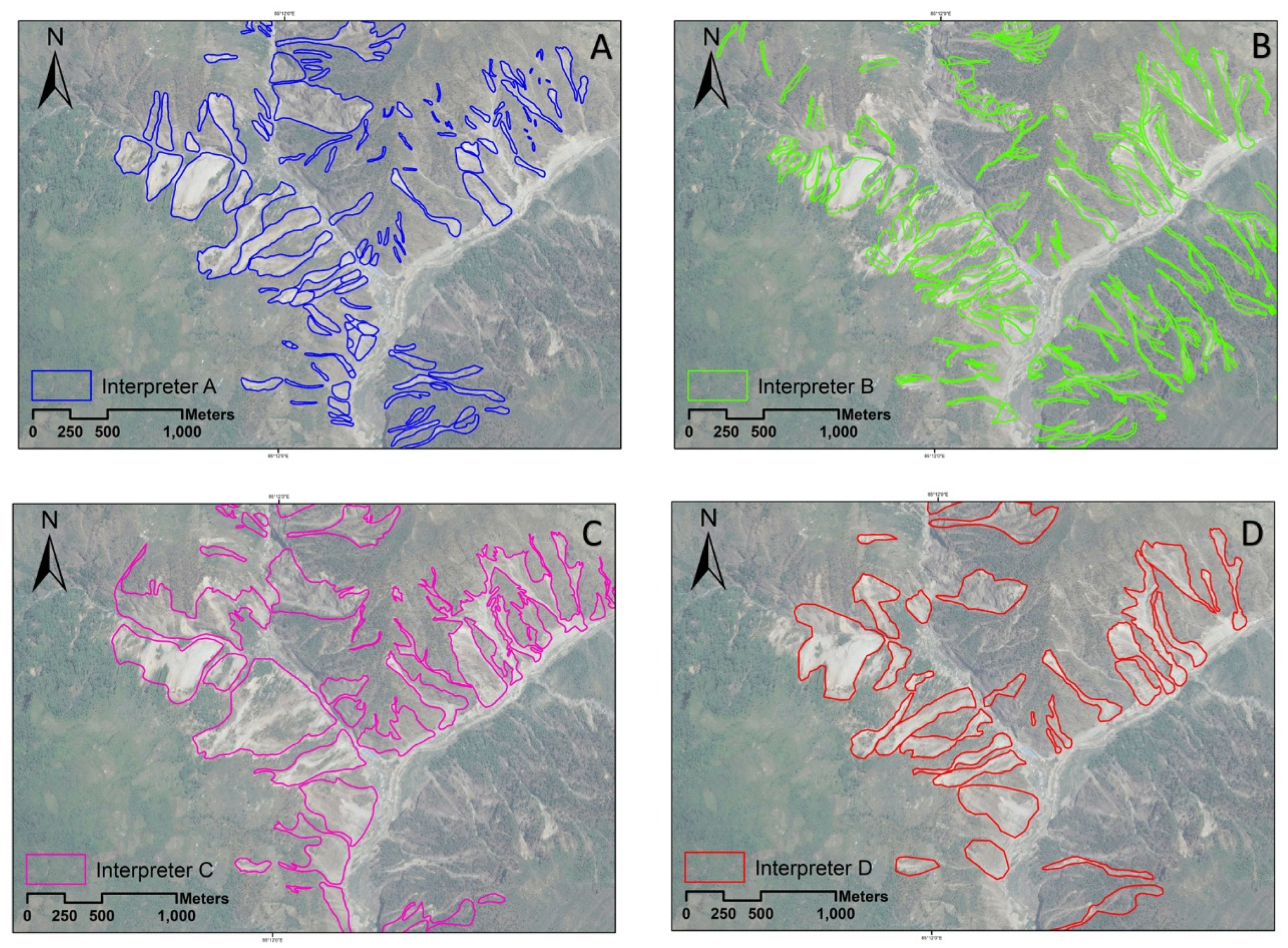
The availability of four independent landslide inventories for the same triggering event in the same geographical area allowed us to quantitatively compare and outline strengths and weaknesses of the methods used to prepare the inventories. The inventory by interpreter B (Figure 10b) portrayed more landslides (498) than the other inventories. This difference was significant, as the other interpreters could not detect most of the smaller landslides visually using Google Earth imagery, which was used to prepare the three inventories by interpreters A, C, and D. The more significant number of landslides in the inventory by interpreter B with the very high-resolution Worldview imagery used for the visual identification of the landslides, compared to the spatial resolution of the satellite imagery used for the other inventories, is explained here. The amalgamation of the landslide information merged multiple very small landslides into a single larger landslide, reducing the total number of the mapped event landslides. Considering only the number of landslides, quantitative identification could not be performed because of both the amalgamation of adjacent landslides and the subjectivity of the landslide extraction process. Many factors caused the amalgamation of landslides in a landslide inventory map. The manual extraction of landslide borders and representation with polygons is a subjective process that is affected by the applied method, the preferences of the experts and interpreters, and how much time and effort are invested into the inventory generating process [61]. Amalgamation is the mapping of nearby smaller landslides as a single polygon, which may lead to possibly severe distortion of the statistical analysis of these inventories. An adjacent landslide polygon is usually described as a single polygon if the runouts or scars overlap in areas. Thus, differentiating between them is difficult. Low image resolution, the working scale, and the contrast between affected and unaffected areas are all other reasons for amalgamation [62]. In some regions, landslides can be very condensed, and several contiguous landslides may join runout areas. Amalgamation is often due to errors resulting from a lack of expertise of the interpreter. It may also happen when landslide inventory mapping is carried out using (semi)-automated classification and change detection based on optical satellite images, e.g., [63].

There are different numbers of mapped landslides for the same area interpreted by different interpreters, which related to the scale of working, applied EO spatial resolution, personal perspective, and the method of mapping that was adopted. Inventory C (Figure 10C) and inventory D (Figure 10D) landslides were mapped using Google Earth imagery; 197 and 336 landslides were mapped, respectively. In Figure 10A, inventory A had 144 landslides for the same common area using Google Earth imagery. Figure 10B shows 498 landslides in inventory B, which was the result of using high-resolution Digital Globe WorldView 2–3 satellite imagery by the author. However, it should be mentioned that very high resolution (VHR) optical satellite imagery can have significant distortions and georeferencing errors in high-relief areas if they are orthorectified using only provided rational polynomial coefficient (RPC) models and not by using manual ground control points (GCPs). Also, this can be more severe, as many of the VHR rapid emergency acquisitions over a disaster area-of-interest can have small incidence angles, thus increasing automatic orthorectification errors. Differences in the mapped outlines of landslides can be due to this. The offset from automatic RPC processing is no less than 5 m for the newer sensors (WorldView 2- 3, Pleiades) and even less for older satellites (GeoEye-1, etc). High mountain relief and low-resolution digital elvetaion model (DEM) used for orthorectification (e.g., Shuttle Radar Topography Mission (SRTM), Advanced Spaceborne Thermal Emission and Reflection Radiometer (ASTER) or Advanced Land Observing Satellite (ALOS) may add more possible errors to these offsets [64].

The results of our mismatch index in this work confirm that the difference between the four-event inventories was significant. However, the mismatch index was in the range of the differences measured by other investigators in previous studies that compared landslide inventories in similar physiographical settings (e.g., [25,52]). In addition to the causes for the mismatch discussed by these investigators, in our test case, the difference was also the result of the period of landslides mapped and of the different spatial resolutions of the satellite imagery. Despite the mismatch index, E, visual inspection of the four inventories revealed a similar spatial distribution of the event landslides in the four landslide maps. This matter was confirmed (i) by the spatial correlation between the four inventories and (ii) by the similarities of the double Pareto density functions for the four inventories (see Figure 10). The results of the power-law exponent of the four analysed inventory ranged from 2.27 to 2.48, which was consistent with the literature that showed that the power-law exponent interval had a central tendency around 2.3–2.5 [55,58].

According to the results of the present study, we conclude that both comparison methods, i.e., the cartographical degree of matching and FAD, are essential for evaluating the quality of landslide inventory productions in terms of their similarities in the total number, area size, and spatial density of landslides. However, the cartographical degree of matching method is suitable more for the evaluation and validation of the location and boundaries of the landslide affected areas. Therefore, the cartographical degree of matching method is essential for landslide extraction/annotation studies, especially those using machine learning models for this aim. The accuracy of the resulting landslide extraction from remote sensing data by using the machine-learning models is directly related to the quality of the training data of landslide inventory datasets [1]. Thus, the cartographical degree of the cartographical matching method plays a vital role in enhancing the accuracy of any landslide extracting studies using machine learning models.

On the other hand, although the FAD is also advantageous for landslide detection studies, it is a crucial method for studies which analyse the landslide areas and their distribution in a case study area. Landslide susceptibility mapping, landslide-prone region analysis, and landslide modeling and risk assessment are considered to be studies, where the FAD method should be considered to evaluate the applied inventory datasets.

For the Gorkha earthquake-affected region in central Nepal, we compared four independent event landslide inventories showing landslides triggered by a high-intensity earthquake that hit the area on 25 April 2015. The first inventory was obtained through the visual interpretation of Google Earth imagery. The second inventory was obtained by exploiting a semi-automatic procedure applied to a VHR resolution worldview satellite imagery. We compared the four inventories by exploiting methods already present in the literature and by proposing new qualitative and quantitative criteria. Comparison of the four independent event inventory maps led to the conclusion that the mismatch between the four inventories was significant but consistent with differences measured by other investigators in similar physiographical areas. The mismatch was attributed to (i) different spatial resolutions of the satellite images, (ii) the amalgamation of smaller landslides into larger landslides while delineating the boundaries of landslides; the minimum landslide area was 35.50 m², which was mapped using VHR resolution worldview satellite imagery, whereas, the landslide mapped using Landsat 8 ETM imagery was 500.53 m², and (iii) the inability of the operator to recognize landslides in shadowed areas. For our future work, we will apply these inventories along with some data-driven models to generate landslide susceptibility maps and compare the resulting susceptibility accuracies.

References

1. Ghorbanzadeh, O.; Blaschke, T.; Gholamnia, K.; Meena, S.R.; Tiede, D.; Aryal, J. Evaluation of Different Machine Learning Methods and Deep-Learning Convolutional Neural Networks for Landslide Detection. Remote Sens. 2019, 11, 196. [Google Scholar] [CrossRef]
2. Meena, S.R.; Mishra, B.K.; Tavakkoli Piralilou, S. A Hybrid Spatial Multi-Criteria Evaluation Method for Mapping Landslide Susceptible Areas in Kullu Valley, Himalayas. Geosciences 2019, 9, 156. [Google Scholar] [CrossRef]
3. Mondini, A.; Viero, A.; Cavalli, M.; Marchi, L.; Herrera, G.; Guzzetti, F. Comparison of event landslide inventories: the Pogliaschina catchment test case, Italy. Nat. Hazards Earth Syst. Sci. 2014, 14, 1749–1759. [Google Scholar] [CrossRef] [Green Version]
4. Dhital, M. Causes and consequences of the 1993 debris flows and landslides in the Kulekhani watershed, central Nepal. In Proceedings of the 3rd International Conference on Debris-Flow Hazards Mitigation: Mechanics, Prediction and Assessment, Davos, Switzerland, 10–12 September 2003; Rickenmann, D., Chen, C.-L., Eds.; Millpress: Rotterdam, The Netherlands, 2003. [Google Scholar]
5. Xu, Q.; Fan, X.M.; Huang, R.Q.; Westen, C.V. Landslide dams triggered by the Wenchuan Earthquake, Sichuan Province, south west China. Bull. Eng. Geol. Environ. 2009, 68, 373–386. [Google Scholar] [CrossRef]
6. Meena, S.R.; Ghorbanzadeh, O.; Blaschke, T. A Comparative Study of Statistics-Based Landslide Susceptibility Models: A Case Study of the Region Affected by the Gorkha Earthquake in Nepal. ISPRS Int. J. Geo-Inf. 2019, 8, 94. [Google Scholar] [CrossRef]
7. Keefer, D.K. Investigating landslides caused by earthquakes—A historical review. Surv. Geophys. 2002, 23, 473–510. [Google Scholar] [CrossRef]
8. Ghorbanzadeh, O.; Blaschke, T. Optimizing Sample Patches Selection of CNN to Improve the mIOU on Landslide Detection. In Proceedings of the 5th International Conference on Geographical Information Systems Theory, Applications and Management: GISTAM, Heraklion, Greece, 3–5 May 2019; Volume 1, p. 8. [Google Scholar] [CrossRef]
9. Harp, E.L.; Keefer, D.K.; Sato, H.P.; Yagi, H. Landslide inventories: The essential part of seismic landslide hazard analyses. Eng. Geol. 2011, 122, 9–21. [Google Scholar] [CrossRef]
10. Damm, B.; Klose, M. The landslide database for Germany: Closing the gap at national level. Geomorphology 2015, 249, 82–93. [Google Scholar] [CrossRef]
11. Guzzetti, F.; Mondini, A.C.; Cardinali, M.; Fiorucci, F.; Santangelo, M.; Chang, K.-T. Landslide inventory maps: New tools for an old problem. Earth-Sci. Rev. 2012, 112, 42–66. [Google Scholar] [CrossRef] [Green Version]
12. Ciampalini, A.; Raspini, F.; Bianchini, S.; Frodella, W.; Bardi, F.; Lagomarsino, D.; Di Traglia, F.; Moretti, S.; Proietti, C.; Pagliara, P. Remote sensing as tool for development of landslide databases: the case of the Messina Province (Italy) geodatabase. Geomorphology 2015, 249, 103–118. [Google Scholar] [CrossRef]
13. Van Westen, C.J.; Ghosh, S.; Jaiswal, P.; Martha, T.R.; Kuriakose, S.L. From landslide inventories to landslide risk assessment; an attempt to support methodological development in India. In Landslide Science and Practice: Landslide Inventory and Susceptibility and Hazard Zoning; Springer: Berlin/Heidelberg, Germany, 2013; Volume 1, pp. 3–20. [Google Scholar]
14. Ghorbanzadeh, O.; Meena, S.R.; Blaschke, T.; Aryal, J. UAV-Based Slope Failure Detection Using Deep-Learning Convolutional Neural Networks. Remote Sens. 2019, 11, 2046. [Google Scholar] [CrossRef]
15. Golovko, D.; Roessner, S.; Behling, R.; Wetzel, H.-U.; Kaufmann, H. GIS-based integration of heterogeneous data for a multi-temporal landslide inventory. In Landslide Science for a Safer Geoenvironment; Springer: Berlin/Heidelberg, Germany, 2014; pp. 799–804. [Google Scholar]
16. Ghorbanzadeh, O.; Feizizadeh, B.; Blaschke, T.; Khosravi, R. Spatially Explicit Sensitivity and Uncertainty Analysis for the landslide risk assessment of the Gas Pipeline Networks. In Proceedings of the 21st AGILE Conference on Geo-Information Science, Lund, Sweden, 12–15 June 2018; pp. 1–7. [Google Scholar]
17. Lahousse, T.; Chang, K.; Lin, Y. Landslide mapping with multi-scale object-based image analysis—A case study in the Baichi watershed, Taiwan. Nat. Hazards Earth Syst. Sci. 2011, 11, 2715–2726. [Google Scholar] [CrossRef]
18. Sansar Raj, M.; Thimmaiah, G.N. Impact of Spatial Resolution of Digital Elevation Model on Landslide Susceptibility Mapping: A case Study in Kullu Valley, Himalayas. Geosciences 2019, 9, 360. [Google Scholar] [CrossRef]
19. Schweigl, J.; Straka, W. Working with Landslide Inventories and Susceptibility Maps in Lower Austria. In Landslide Science and Practice: Landslide Inventory and Susceptibility and Hazard Zoning; Margottini, C., Canuti, P., Sassa, K., Eds.; Springer: Berlin/Heidelberg, Germany, 2013; Volume 1, pp. 43–50. [Google Scholar]
20. Borghuis, A.M.; Chang, K.; Lee, H.Y. Comparison Between Automated and Manual Mapping of Typhoon-triggered Landslides from SPOT-5 Imagery. Int. J. Remote Sens. 2007, 28, 1843–1856. [Google Scholar] [CrossRef]
21. Danneels, G.; Pirard, E.; Havenith, H.-B. Automatic landslide detection from remote sensing images using supervised classification methods. In Proceedings of the IEEE International Geoscience and Remote Sensing Symposium (IGARSS 2007), Barcelona, Spain, 23–28 July 2007; pp. 3014–3017. [Google Scholar]
22. Keyport, R.N.; Oommen, T.; Martha, T.R.; Sajinkumar, K.; Gierke, J.S. A comparative analysis of pixel-and object-based detection of landslides from very high-resolution images. Int. J. Appl. Earth Obs. Geoinf. 2018, 64, 1–11. [Google Scholar] [CrossRef]
23. Pellicani, R.; Spilotro, G. Evaluating the quality of landslide inventory maps: Comparison between archive and surveyed inventories for the Daunia region (Apulia, Southern Italy). Bull. Eng. Geol. Environ. 2015, 74, 357–367. [Google Scholar] [CrossRef]
24. Fan, X.; Scaringi, G.; Korup, O.; West, A.J.; van Westen, C.J.; Tanyas, H.; Hovius, N.; Hales, T.C.; Jibson, R.W.; Allstadt, K.E.; et al. Earthquake-induced chains of geologic hazards: Patterns, mechanisms, and impacts. Rev. Geophys. 2019. [Google Scholar] [CrossRef]
25. Galli, M.; Ardizzone, F.; Cardinali, M.; Guzzetti, F.; Reichenbach, P. Comparing landslide inventory maps. Geomorphology 2008, 94, 268–289. [Google Scholar] [CrossRef]
26. Guzzetti, F.; Cardinali, M.; Reichenbach, P.; Carrara, A. Comparing landslide maps: A case study in the upper Tiber River basin, central Italy. Environ. Manag. 2000, 25, 247–263. [Google Scholar] [CrossRef]
27. Keefer, D.K. Landslides caused by earthquakes. Geol. Soc. Am. Bull. 1984, 95, 406–421. [Google Scholar] [CrossRef]
28. Rodríguez, C.E.; Bommer, J.J.; Chandler, R.J. Earthquake-induced landslides: 1980–1997. Soil Dyn. Earthq. Eng. 1999, 18, 325–346. [Google Scholar] [CrossRef]
29. Keefer, D.K. Statistical analysis of an earthquake-induced landslide distribution — the 1989 Loma Prieta, California event. Eng. Geol. 2000, 58, 231–249. [Google Scholar] [CrossRef]
30. Esposito, E.; Porfido, S.; Simonelli, A.L.; Mastrolorenzo, G.; Iaccarino, G. Landslides and other surface effects induced by the 1997 Umbria–Marche seismic sequence. Eng. Geol. 2000, 58, 353–376. [Google Scholar] [CrossRef]
31. Serva, L.; Vittori, E.; Comerci, V.; Esposito, E.; Guerrieri, L.; Michetti, A.M.; Mohammadioun, B.; Mohammadioun, G.C.; Porfido, S.; Tatevossian, R.E. Earthquake Hazard and the Environmental Seismic Intensity (ESI) Scale. Pure Appl. Geophys. 2016, 173, 1479–1515. [Google Scholar] [CrossRef]
32. Guerrieri, L.; Michetti, A.; Reicherter, K.; Serva, L.; Silva, P.; Audemard, F.; Azuma, T.; Baiocco, F.; Baize, S.; Blumetti, A. Earthquake environmental effect for seismic hazard assessment: The ESI intensity scale and the EEE catalogue. Mem. descr. Carta Geol. D’italia 2015, 97, 11–20. [Google Scholar]
33. Lekkas, E.L. The 12 May 2008 Mw 7.9 Wenchuan, China, Earthquake: Macroseismic Intensity Assessment Using the EMS-98 and ESI 2007 Scales and Their Correlation with the Geological Structure. Bull. Seismol. Soc. Am. 2010, 100, 2791–2804. [Google Scholar] [CrossRef]
34. Chunga, K.; Livio, F.A.; Martillo, C.; Lara-Saavedra, H.; Ferrario, M.F.; Zevallos, I.; Michetti, A.M. Landslides Triggered by the 2016 Mw 7.8 Pedernales, Ecuador Earthquake: Correlations with ESI-07 Intensity, Lithology, Slope and PGA-h. Geosciences 2019, 9, 371. [Google Scholar] [CrossRef]
35. Ferrario, M.F. Landslides triggered by multiple earthquakes: insights from the 2018 Lombok (Indonesia) events. Nat. Hazards 2019, 98, 575–592. [Google Scholar] [CrossRef]
36. Xu, C.; Xu, X.; Yao, X.; Dai, F. Three (nearly) complete inventories of landslides triggered by the May 12, 2008 Wenchuan Mw 7.9 earthquake of China and their spatial distribution statistical analysis. Landslides 2014, 11, 441–461. [Google Scholar] [CrossRef]
37. Alessio, G.; Alfonsi, L.; Brunori, C.A.; Burrato, P.; Casula, G.; Cinti, F.R.; Civico, R.; Colini, L.; Cucci, L.; De Martini, P.M.; et al. Technologies and new approaches used by the INGV EMERGEO Working Group for real-time data sourcing and processing during the Emilia Romagna (northern Italy) 2012 earthquake sequence. Ann. Geophys. 2012, 55. [Google Scholar] [CrossRef]
38. Civico, R.; Pucci, S.; Villani, F.; Pizzimenti, L.; De Martini, P.M.; Nappi, R. Surface ruptures following the 30 October 2016 Mw 6.5 Norcia earthquake, central Italy. J. Maps 2018, 14, 151–160. [Google Scholar] [CrossRef]
39. Villani, F.; Civico, R.; Pucci, S.; Pizzimenti, L.; Nappi, R.; De Martini, P.M.; The Open EMERGEO Working Group. A database of the coseismic effects following the 30 October 2016 Norcia earthquake in Central Italy. Sci. Data 2018, 5, 180049. [Google Scholar] [CrossRef] [PubMed] [Green Version]
40. Tanyaş, H.; van Westen, C.J.; Allstadt, K.E.; Anna Nowicki Jessee, M.; Görüm, T.; Jibson, R.W.; Godt, J.W.; Sato, H.P.; Schmitt, R.G.; Marc, O.; et al. Presentation and Analysis of a Worldwide Database of Earthquake-Induced Landslide Inventories. J. Geophys. Res. Earth Surf. 2017, 122, 1991–2015. [Google Scholar] [CrossRef] [Green Version]
41. Tsou, C.-Y.; Chigira, M.; Higaki, D.; Sato, G.; Yagi, H.; Sato, H.P.; Wakai, A.; Dangol, V.; Amatya, S.C.; Yatagai, A. Topographic and geologic controls on landslides induced by the 2015 Gorkha earthquake and its aftershocks: an example from the Trishuli Valley, central Nepal. Landslides 2018, 15, 953–965. [Google Scholar] [CrossRef]
42. Regmi, A.D.; Dhital, M.R.; Zhang, J.-Q.; Su, L.-J.; Chen, X.-Q. Landslide susceptibility assessment of the region affected by the 25 April 2015 Gorkha earthquake of Nepal. J. Mt. Sci. 2016, 13, 1941–1957. [Google Scholar] [CrossRef]
43. Ni, J.; Barazangi, M. Seismotectonics of the Himalayan collision zone: Geometry of the underthrusting Indian plate beneath the Himalaya. J. Geophys. Res. Solid Earth 1984, 89, 1147–1163. [Google Scholar] [CrossRef]
44. Roback, K.; Clark, M.K.; West, A.J.; Zekkos, D.; Li, G.; Gallen, S.F.; Chamlagain, D.; Godt, J.W. The size, distribution, and mobility of landslides caused by the 2015 Mw7. 8 Gorkha earthquake, Nepal. Geomorphology 2018, 301, 121–138. [Google Scholar] [CrossRef]
45. Gnyawali, K.R.; Maka, S.; Adhikari, B.R.; Chamlagain, D.; Duwal, S.; Dhungana, A.R. Spatial implications of earthquake induced landslides triggered by the April 25 Gorkha earthquake Mw 7.8: preliminary analysis and findings. In Proceedings of the International Conference on Earthquake Engineering and Post Disastor Reconstruction Planning, Bhaktapur, Nepal, 24–26 April 2016. [Google Scholar]
46. Robinson, T.R.; Rosser, N.J.; Densmore, A.L.; Williams, J.G.; Kincey, M.E.; Benjamin, J.; Bell, H.J. Rapid post-earthquake modelling of coseismic landsliding intensity and distribution for emergency response decision support. Nat. Hazards Earth Syst. Sci. 2017, 17, 1521–1540. [Google Scholar] [CrossRef]
47. Cruden, D.M.; Varnes, D.J. Landslide Types and Processes. Spec. Rep. Natl. Res. Counc. Transp. Res. Board 1996, 247, 76. [Google Scholar]
48. Valagussa, A.; Frattini, P.; Crosta, G.; Valbuzzi, E. Pre and post 2015 Nepal earthquake landslide inventories. In Landslides and Engineered Slopes. Experience, Theory and Practice; CRC Press: Boca Raton, FL, USA, 2016; pp. 1957–1964. [Google Scholar]
49. Martha, T.R.; Roy, P.; Mazumdar, R.; Govindharaj, K.B.; Kumar, K.V. Spatial characteristics of landslides triggered by the 2015 M w 7.8 (Gorkha) and M w 7.3 (Dolakha) earthquakes in Nepal. Landslides 2017, 14, 697–704. [Google Scholar] [CrossRef]
50. Meena, S.R.; Mavrouli, O.; Westen, C.J. Web based landslide management system for Nepal. In Proceedings of the 33rd Himalaya-Karakorum-Tibet Workshop (HKT), Lausanne, Switzerland, 10–12 September 2018; pp. 109–110. [Google Scholar]
51. Kargel, J.; Leonard, G.; Shugar, D.H.; Haritashya, U.; Bevington, A.; Fielding, E.; Fujita, K.; Geertsema, M.; Miles, E.; Steiner, J. Geomorphic and geologic controls of geohazards induced by Nepal’s 2015 Gorkha earthquake. Science 2016, 351, aac8353. [Google Scholar] [CrossRef] [PubMed]
52. Carrara, A. Uncertainty in evaluating landslide hazard and risk. In Prediction and Perception of Natural Hazards; Springer: Berlin/Heidelberg, Germany, 1993; pp. 101–109. [Google Scholar]
53. Malamud, B.D.; Turcotte, D.L.; Guzzetti, F.; Reichenbach, P. Landslide inventories and their statistical properties. Earth Surf. Process. Landf. 2004, 29, 687–711. [Google Scholar] [CrossRef]
54. Guzzetti, F.; Malamud, B.D.; Turcotte, D.L.; Reichenbach, P. Power-law correlations of landslide areas in central Italy. Earth Planet. Sci. Lett. 2002, 195, 169–183. [Google Scholar] [CrossRef]
55. Stark, C.P.; Guzzetti, F. Landslide rupture and the probability distribution of mobilized debris volumes. J. Geophys. Res. Earth Surf. 2009, 114, 1–16. [Google Scholar] [CrossRef]
56. Tanyaş, H.; van Westen, C.J.; Allstadt, K.E.; Jibson, R.W. Factors controlling landslide frequency—Area distributions. Earth Surf. Process. Landf. 2019, 44, 900–917. [Google Scholar] [CrossRef]
57. Stark, C.P.; Hovius, N. The characterization of landslide size distributions. Geophys. Res. Lett. 2001, 28, 1091–1094. [Google Scholar] [CrossRef]
58. Van Den Eeckhaut, M.; Poesen, J.; Govers, G.; Verstraeten, G.; Demoulin, A. Characteristics of the size distribution of recent and historical landslides in a populated hilly region. Earth Planet. Sci. Lett. 2007, 256, 588–603. [Google Scholar] [CrossRef]
59. Guthrie, R.H.; Evans, S.G. Analysis of landslide frequencies and characteristics in a natural system, coastal British Columbia. Earth Surf. Process. Landf. 2004, 29, 1321–1339. [Google Scholar] [CrossRef]
60. Malamud, B.D.; Turcotte, D.L.; Guzzetti, F.; Reichenbach, P. Landslides, earthquakes, and erosion. Earth Planet. Sci. Lett. 2004, 229, 45–59. [Google Scholar] [CrossRef]
61. Soeters, R.; van Westen, C.J. Slope instability recognition, analysis, and zonation. Landslides Investig. Mitig. 1996, 247, 129–177. [Google Scholar]
62. Marc, O.; Hovius, N. Amalgamation in landslide maps: effects and automatic detection. Nat. Hazards Earth Syst. Sci. 2015, 15, 723–733. [Google Scholar] [CrossRef] [Green Version]
63. Martha, T.R.; Kerle, N.; Jetten, V.; van Westen, C.J.; Kumar, K.V. Characterising spectral, spatial and morphometric properties of landslides for semi-automatic detection using object-oriented methods. Geomorphology 2010, 116, 24–36. [Google Scholar] [CrossRef]
64. Tang, C.; Van Westen, C.J.; Tanyas, H.; Jetten, V.G. Analysing post-earthquake landslide activity using multi-temporal landslide inventories near the epicentral area of the 2008 Wenchuan earthquake. Nat. Hazards Earth Syst. Sci. 2016, 16, 2641–2655. [Google Scholar] [CrossRef] [Green Version]
Figure 1. Area covered by the different investigators during mapping landslide inventories of the 2015 Gorkha earthquake.
Geosciences 09 00437 g001
Figure 2. Landslide mapped after the 2015 Gorkha earthquake for the affected region. (A) Inventory A, (B) inventory B, (C) inventory C, and (D) inventory D.
Geosciences 09 00437 g002
Figure 3. Landslide inventory densities per km² for the Gorkha event. (A) Inventory A, (B) inventory B, (C) inventory C, and (D) inventory D.
Geosciences 09 00437 g003
Figure 4. (A) Example of a union with features within a feature class that overlaps. (B) Example of an intersection with a feature within a feature class that overlaps.
Geosciences 09 00437 g004
Figure 5. Mapping by different interpreters for the Gorkha earthquake of the same landslides. (A,B) represent examples of the mapped landslides.
Geosciences 09 00437 g005
Figure 6. Pairwise comparison of inventories mapped by different interpreters.
Geosciences 09 00437 g006
Figure 7. Comparison of inventories mapped by different interpreters.
Geosciences 09 00437 g007
Figure 8. Schematic representation of the main components of a non-cumulative frequency area distribution (FAD) for a landslide inventory.
Geosciences 09 00437 g008
Figure 9. Landslide frequency size distribution, representing the dependence of landslide probability density p on the landslide area.
Geosciences 09 00437 g009
Figure 10. Effect of amalgamation for the same area mapped by four different people in the area near the Trishuli river, (A) Inventory A, (B) inventory B, (C) inventory C, and (D) inventory D.
Geosciences 09 00437 g010