The Concept of Geodetic Analyses of the Measurement Results Obtained by Hydrostatic Leveling

Abstract

The article discusses the issue of hydrostatic leveling. Its application is presented in structural health monitoring systems in order to determine vertical displacements of controlled points. Moreover, the article includes a complete computation scheme that utilizes the estimation from observation differences, allowing the elimination of the influence of individual sensors’ systematic errors. The authors suggest two concepts of processing the measurement results depending on the sensors’ connection method. Additionally, the second concept is extended by the elements allowing the prediction of the displacements by means of Kalman filtering.

1. Introduction

Hydrostatic leveling is mentioned as one of the oldest methods used to determine the height difference between controlled points. This method is mainly applied in measurements where highly accurate and highly reliable final results are necessary. However, it can be also used when geometric or trigonometric leveling is difficult to carry out. A relevant example is provided by the measurements made in 1939—hydrostatic leveling enabled establishing leveling connection between the Danish and Swedish height systems [1].

Hydrostatic leveling is often implemented in structural health monitoring (SHM) systems because of its high accuracy. The SHM systems with hydrostatic leveling were applied in objects such as dams [2], embankments [3], and metro tunnels; the latter systems are established during tunnel excavation [4]. Wei et al. [5] presented an application of hydrostatic leveling to determine vertical displacements of the SLS (Swiss Light Source) storage ring girders. Morishita and Ikegami [6] explained the slow-ground-motion monitoring system for the J-PARC (Japan Proton Accelerator Research Complex) linac, while Zhang et al. [7] focused on processing the power transmission tower vertical displacements. Other examples of hydrostatic leveling systems address the European Synchrotron Radiation Facility (ESRF) [8] and the TT1 tunnel at CERN (European Organization for Nuclear Research) [9]. The review above shows an enormous variety of objects involving hydrostatic leveling for displacement study.

The paper utilizes the adopted classification of hydrostatic leveling systems of Wilde et al. [10]. Thus, open and closed leveling systems are listed here. The open leveling systems are characterized by the simplest design in which the fluid freely flows between the sensors and is directly exposed to the environment. Contrary to open leveling systems, the closed leveling systems are characterized by absolute tightness of the sensors filled with working fluid, in order to reduce the effect of external factors on the hydrostatic leveling system performance.

In further analysis, the authors focus on introducing two concepts of processing the measurement results of the open leveling system. Concept I is based on the assumption that each sensor is connected directly to the expansion tank. Concept II, however, presupposes that sensors are mutually interconnected. Additionally, the second concept is supplemented by the Kalman filtering method that additionally enables the prediction of the identified displacements. The idea of hydrostatic leveling is based on the well-known Bernoulli equation in the following form [11]:

$$\frac{1}{2}\rho {\overline{v}}^2+p+\rho gZ=\mathrm{const},$$

(1)

where: $\rho$—fluid density, $\overline{v}$—fluid velocity, $p$—hydrostatic pressure, $g$—standard acceleration of gravity, $Z$—fluid column height.

Assuming that for the majority of hydrostatic leveling systems the fluid is at rest ($\overline{v}=0$), Equation (1) takes the simplified form

$$p+\rho gZ=\mathrm{const}.$$

(2)

Besides the Bernoulli equation, this kind of leveling is also based on the principle of equal fluid-level in the communicating vessels. As a result, relation (2) can be used to determine the height difference between two sensors involved in the measurement of the height of fluid column Z. Therefore, the relation schematically illustrated in Figure 1 can be written as follows:

$$p_1+{\rho }_1{g}_1{Z}_1=p_2+{\rho }_2{g}_2\left(Z_2+d{Z}_{12}\right),$$

(3)

where: subscript $1,2$—identification of first/second sensor, $d{Z}_{12}$—height difference between the fulcrums of two sensors.

After converting Equation (3), the result becomes

$$d{Z}_{12}=\frac{p_1+{\rho }_1{g}_1{Z}_1-p_2-{\rho }_2{g}_2{Z}_2}{{\rho }_2{g}_2}.$$

(4)

Considering additional assumptions regarding equal hydrostatic pressure, fluid density, and standard gravity in both vessels ($p_1=p_2,{\rho }_1={\rho }_2,g_1=g_2$), the height difference between two sensors may be derived from the relation

$$d{Z}_{12}=Z_1-Z_2.$$

(5)

This, however, is a simplified version of the hydrostatic leveling relation.

Observations collected through hydrostatic leveling may be affected by measurement errors, possibly caused by:

• Density variation of the fluid filling the sensor connecting pipe which is a function of temperature $T$ and pressure $p$, $\rho =f(T,p)$. It is difficult or even impossible to assess precisely the density variations;
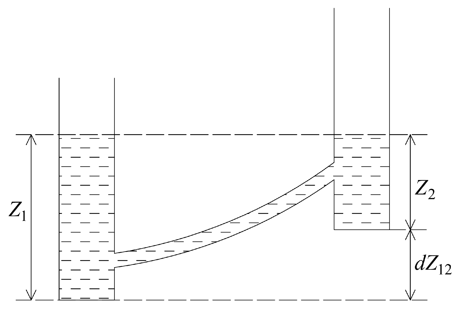
• Errors in determining the exact fluid column height in sensors;
• The changes of atmospheric pressure;
• Standard acceleration due to gravity changes;
• A tidal phenomenon (low and high tides).

The errors mentioned above may trigger systematic errors s.

2. Materials and Methods

The aim of the paper is presenting the concept of geodetic processing of the hydrostatic leveling results. A number of relations are required to reach the final solution. It is assumed that ${\mathrm{Z}}_i^{(1)}$ is the fluid column height in sensor no. i ($i=1,\dots ,n$) in the initial epoch and ${\mathrm{Z}}_i^{(2)}$ is the fluid column height in the actual epoch.

Equation (5) for the initial epoch can be presented as follows:

$$d{Z}_j^{(1)}=Z_B^{(1)}-Z_F^{(1)},$$

(6)

where: $Z_B^{(1)}$—backward reading on sensor, $Z_F^{(1)}$—forward reading on sensor, j—the number of height differences ($j=1,\dots ,m$).

Similarly, Equation (5) in the actual epoch takes the form

$$d{Z}_j^{(2)}=Z_B^{(2)}-Z_F^{(2)},$$

(7)

where: $Z_B^{(2)}$—backward reading on sensor, $Z_F^{(2)}$—forward reading on sensor.

When carrying out the hydrostatic leveling measurements, we can expect that the readings of the fluid column height may be affected by systematic errors. Consequently, the following can be noted:

$$\begin{array}{l}{\tilde{Z}}_B^{(1)}=Z_B^{(1)}+s_i^{(1)}\\ {\tilde{Z}}_F^{(1)}=Z_F^{(1)}+s_{i+1}^{(1)}\end{array}$$

(8)

where $s_i$—sensor no. i systematic error.

Thus:

$$d{\tilde{Z}}_j^{(1)}=\left(Z_B^{(1)}+s_i^{(1)}\right)-\left(Z_F^{(1)}+s_{i+1}^{(1)}\right).$$

(9)

A similar relation can be determined for readings in the actual epoch:

$$d{\tilde{Z}}_j^{(2)}=\left(Z_B^{(2)}+s_i^{(2)}\right)-\left(Z_F^{(2)}+s_{i+1}^{(2)}\right),$$

(10)

where:

$$\begin{array}{l}{\tilde{Z}}_B^{(2)}=Z_B^{(2)}+s_i^{(2)}\\ {\tilde{Z}}_F^{(2)}=Z_F^{(2)}+s_{i+1}^{(2)}\end{array}$$

(11)

In order to reject the impact of systematic errors on final results of the estimation, the method of observation differences may be applied as

$$\begin{array}{l}d{z}_j=d{\tilde{Z}}_j^{(2)}-d{\tilde{Z}}_j^{(1)}=\left(Z_B^{(2)}+s_i^{(2)}\right)-\left(Z_F^{(2)}+s_{i+1}^{(2)}\right)-\left(Z_B^{(1)}+s_i^{(1)}\right)+\left(Z_F^{(1)}+s_{i+1}^{(1)}\right)\\ \hspace{1em}\hspace{1em}\hspace{1em}\hspace{1em}\hspace{1em}\hspace{0.17em}d{z}_j=\left(d{Z}^{(2)}+d{s}^{(2)}\right)-\left(d{Z}^{(1)}+d{s}^{(1)}\right)\end{array}$$

(12)

where: $d{s}^{(2)}=s_i^{(2)}-s_{i+1}^{(2)}$ and $d{s}^{(1)}=s_i^{(1)}-s_{i+1}^{(1)}$.

It is important that none of the analyzed papers describe the estimation based on observation differences to determine the sensor displacements.

Based on the assumption that systematic errors of individual sensors are constant over time ($s_i^{(2)}=s_i^{(1)}$ and $s_{i+1}^{(2)}=s_{i+1}^{(1)}$), the relation $d{s}^{(2)}-d{s}^{(1)}=0$ is obtained. Hence the equation of pseudo-observation ($d{z}_j$) takes the form

$$d{z}_j=d{Z}_j^{(2)}-d{Z}_j^{(1)}.$$

(13)

Assuming that $u_B$ means the back sensor displacement and $u_F$ means the forward sensor displacement, the following formula can be applied:

$$u_B+d{z}_j+v_j=u_F.$$

(14)

Converting relation (14), the equation of pseudo-observation corrections reads

$$v_j=u_F-u_B-d{z}_j.$$

(15)

The equation above can be written in the matrix notation as follows:

$$v=Au+y,$$

(16)

where: $v={[v_1,\dots ,v_m]}^T$, $u={[u_1,\dots , u_n]}^T$, $y={[-d{z}_1,\dots ,-d{z}_m]}^T$, and $A$ is a known coefficient matrix.

In the present experimental course, the measurement results were obtained by means of the open leveling system. In both open and closed leveling systems, there were no redundant observations. Thus, the achieved results are unambiguous and there is no need to apply the optimization task written below:

$$\begin{array}{l}\varphi \left(u\right)=v^{T}Pv\to \min \\ v=Au+y\\ C_y={\sigma }_0^2{Q}_y\end{array}$$

(17)

where: $P=Q_y{}^{-1}, Q_y=P^{-1}$($P$—weight matrix, $Q_y$—cofactor matrix of measurement results).

As no redundant observations appear, consequently the correction values equal zero ($v=0$). Therefore, Equation (16) can be applied in the form of $Au+y=0$, and so

$$u=-A^{-1}y.$$

(18)

In order to assess the accuracy of computation results (in this case the displacement $u_i$ of each controlled point—sensor), the propagation law of cofactors can be used as follows:

$$Q=D{Q}_y{D}^T.$$

(19)

Assuming that $D=A^{-1}$ and $Q_y=P^{-1}$, the cofactor matrix $Q_u$ may be computed as

$$Q_u=A^{-1}{P}^{-1}{\left(A^{-1}\right)}^T={\left(A^{T}PA\right)}^{-1}.$$

(20)

The elements of the weight matrix $P$ are determined further on. Applying the error propagation law for two sensors (notation: 1, 2) to relation (4), the following outcome is obtained:

$$\begin{array}{l}{m}_{d{Z}_{12}}^2={\left(\frac{\partial d{Z}_{12}}{\partial p_1}\right)}^2{m}_p^2{}_{{}_1}+{\left(\frac{\partial d{Z}_{12}}{\partial {\rho }_1}\right)}^2{m}_{{\rho }_1}^2+{\left(\frac{\partial d{Z}_{12}}{\partial g_1}\right)}^2{m}_{g_1}^2+{\left(\frac{\partial d{Z}_{12}}{\partial Z_1}\right)}^2{m}_{Z_1}^2+{\left(\frac{\partial d{Z}_{12}}{\partial p_2}\right)}^2{m}_p^2{}_{{}_2}+\\ +{\left(\frac{\partial d{Z}_{12}}{\partial {\rho }_2}\right)}^2{m}_{{\rho }_2}^2+{\left(\frac{\partial d{Z}_{12}}{\partial g_2}\right)}^2{m}_{g_2}^2+{\left(\frac{\partial d{Z}_{12}}{\partial Z_2}\right)}^2{m}_{Z_2}^2\end{array}$$

(21)

or, in a simplified form, corresponding to relation (5):

$$m_{d{Z}_{12}}^2={\left(\frac{\partial d{Z}_{12}}{\partial Z_1}\right)}^2{m}_{Z_1}^2+{\left(\frac{\partial d{Z}_{12}}{\partial Z_2}\right)}^2{m}_{Z_2}^2.$$

(22)

Based on relations (21) or (22), the mean square error values of height difference between two sensors may be obtained, both in the initial and actual epoch. The functional model $d{z}_j=d{Z}_j^{(2)}-d{Z}_j^{(1)}$ applied in the paper (described by Equation (13)) addresses the observation differences made in two epochs, therefore $m_{d{z}_j}^2$ can be specified as follows:

$$m_{d{z}_j}^2=m_{d{Z}_j^{(2)}}^2+m_{d{Z}_j^{(1)}}^2,$$

(23)

where: $m_{d{Z}_j^{(1)}}^2$,$m_{d{Z}_j^{(2)}}^2$—the mean square errors of height difference between two sensors computed from relation (21) or (22), in the initial and actual epochs, respectively.

While the mean error values are known, the weight of individual pseudo-observations may be derived ($p_j=\frac{1}{m_{d{z}_j}^2}$), and the weight matrix is given as $P=\mathrm{Diag}\left(p_1,\dots ,p_m\right)$.

The performed analysis utilizes the Kalman filtering method. General assumptions regarding this method and its application in geodetic measurement result processing are discussed in [12,13,14,15,16]. In the paper, Kalman filtering is implemented to predict sensor displacements. In order to apply this methodology in the conducted analysis, it is essential to define a valid kinematic or dynamic model of the investigated object. Let us assume a general kinematic model including position, velocity, and acceleration in the form of

$$\begin{array}{l}{u}_{k+1}=u_k+{\upsilon }_k\Delta t+\frac{1}{2}{a}_k\Delta t^2+e_u\\ {\upsilon }_{k+1}={\upsilon }_k +\hspace{0.17em}{a}_k\Delta t\hspace{1em}\hspace{0.17em}\hspace{0.17em}+e_{\upsilon }\\ a_{k+1}= \hspace{1em}\hspace{1em}\hspace{1em}\hspace{0.17em}\hspace{0.17em}\hspace{0.17em}\hspace{1em}+\hspace{0.17em}{a}_k\hspace{1em}\hspace{1em}\hspace{0.17em} +e_a\end{array}$$

(24)

where:

• $u_k$—vector of displacements at epoch k,
• ${\upsilon }_k$—velocity vector at epoch k,
• $a_k$—acceleration vector at epoch k,
• subscript ${}_{k+1}$—values denotes the prediction results,
• $\Delta t$—time interval between epochs k and k+1 ($\Delta t=t_{k+1}-t_k$), and
• $e_u$, $e_{\upsilon }$, $e_a$—vectors of random disturbances, due to displacements, velocity, and acceleration at epoch k, respectively.

Assuming that ${\overline{X}}_{k+1}={\left[{\overline{u}}_{k+1}, {\overline{\upsilon }}_{k+1},{\overline{a}}_{k+1}\right]}^T$ is a prediction state vector, ${\Phi }_{k/k+1}$ is a transition matrix between states at epochs k and k+1, $X_k={\left[u_k, {\upsilon }_k,a_k\right]}^T$ is a state vector at epoch k, and $e={\left[e_u, e_{\upsilon },e_a\right]}^T$ is a vector of random disturbances, the relation (24) may be defined as follows (we assume that the expected value $E\left(e\right)=0$):

$${\overline{X}}_{k+1}={\Phi }_{k/k+1}{X}_k,$$

(25)

where the transition matrix takes the form ${\Phi }_{k/k+1}=\left[\begin{array}{ccc}1& \Delta t& \Delta t^2/2\\ 0& 1& \Delta t\\ 0& 0& 1\end{array}\right]$.

In case of a computed prediction state vector ${\overline{X}}_{k+1}$ described by dependence (25), the covariance matrix $C_{{\overline{X}}_{k+1}}$ is defined as follows:

$$C_{{\overline{X}}_{k+1}}={\Phi }_{k/k+1}{C}_{X_k}{\Phi }_{k/k+1}^T+C_e.$$

(26)

Kalman filtering enables simultaneous adjustment of the information obtained from prediction and observation on sensors. Thus, assuming that $A_{k+1}$ is a known coefficient matrix at epoch k+1, $v_{{\overline{X}}_{k+1}}$ is a vector of corrections for prediction at epoch k+1, and ${\overline{v}}_{k+1}$ is a vector of measurement residuals (called innovation) at epoch k+1, the system of observation equations can be presented in the form

$$v_{k+1}=A_{k+1}{v}_{{\overline{X}}_{k+1}}+{\overline{v}}_{k+1}.$$

(27)

The weight matrix of innovation $P_{{\overline{v}}_{k+1}}$ required for further consideration may be derived from the relation

$$P_{{\overline{v}}_{k+1}}={\left(P_{y_{k+1}}^{-1}+A_{k+1}{P}_{{\overline{X}}_{k+1}}^{-1}{A}_{k+1}^T\right)}^{-1},$$

(28)

where:

$P_{y_{k+1}}^{}$—weight matrix of observations at epoch k+1 and $P_{{\overline{X}}_{k+1}}^{-1}=C_{{\overline{X}}_{k+1}}$.

It allows the computation of the two dedicated gain matrices (gain matrix for observations $K_{y_{k+1}}^{}$ and Kalman gain matrix $K_{{\overline{X}}_{k+1}}$) according to the following formulas:

$$K_{y_{k+1}}^{}=P_{y_{k+1}}^{-1}{P}_{{\overline{v}}_{k+1}}$$

(29)

$$K_{{\overline{X}}_{k+1}}^{}=-P_{{\overline{X}}_{k+1}}^{-1}{A}_{k+1}^T{P}_{{\overline{v}}_{k+1}}.$$

(30)

Based on relation (29), there may be obtained the corrections for observations $y_{k+1}$ made at epoch k+1:

$$v_{k+1}=K_{y_{k+1}}^{}{\overline{v}}_{k+1},$$

(31)

and consequently, the vector of adjusted observations in the following form:

$$Y_{k+1}=y_{k+1}+v_{k+1}.$$

(32)

The corrections for prediction should be determined similarly:

$$v_{{\overline{X}}_{k+1}}^{}=K_{{\overline{X}}_{k+1}}^{}{\overline{v}}_{k+1}.$$

(33)

Then, the state vector at epoch k+1 is given by

$$X_{k+1}={\overline{X}}_{k+1}+v_{{\overline{X}}_{k+1}}^{}.$$

(34)

The covariance matrix corresponding to the state vector $X_{k+1}$ described by the relation (34), can be written in the form

$$C_{X_{k+1}}=\left(I+K_{{\overline{X}}_{k+1}}{A}_{k+1}\right)P{\hspace{0.17em}}_{{\overline{X}}_{k+1}}^{-1},$$

(35)

where: $I$—unit matrix.

3. Results

The practical example introduces measurement results of the open levelling system without a gas reference system. An inquiry involving a five-sensor geodetic network is presented below. However, the computation scheme is similar for networks composed of a larger number of sensors. The sensors’ location (for concept II) is shown schematically in Figure 2. In the presented leveling system, the expansion tank also acts as a reference sensor.

Table 1. The readings of the fluid column height on sensors.

Sensor Name	Reading in [mm]
	Initial Epoch	Actual Epoch
expansion tank/ reference sensor	5.1	45.4
sensor no. 1	66.8	101.4
sensor no. 2	53.3	94.7
sensor no. 3	48.0	90.0
sensor no. 4	38.4	80.7
sensor no. 5	43.4	85.4

includes the readings of the fluid column height obtained on each sensor in both measuring epochs.

Further computational stages were carried out according to the two concepts of processing the measurement results, according to the sensors connection method:

Concept I—each sensor is connected directly to the expansion tank,

Concept II—sensors are connected in series and displacement prediction using Kalman filtering is implemented.

The displacement prediction by means of Kalman filtering may be implemented in both presented concepts. However, after performing analyses for the purposes of this paper it was decided to present the prediction on the example of concept II.

3.1. Concept I

Concept I is based on height differences between each sensor and the expansion tank (the reference sensor). The scheme of sensor location for concept I is shown in Figure 3. The height difference values in initial and actual epochs ($d{Z}^{(1)}$ and $d{Z}^{(2)}$), as well as the difference of two height differences ($d{z}_j$), are shown in

Table 2. The input data for concept I.

$\mathbf{Height} \mathbf{Difference} \mathit{d}{\mathit{Z}}_{\mathit{j}}$	Initial Epoch [mm]	Actual Epoch [mm]	$\mathit{d}{\mathit{z}}_{\mathit{j}} \left[\mathbf{mm}\right]$
$j=ref.-no.\hspace{0.17em}1$	−61.7	−56.0	5.7
$j=ref.-no.\hspace{0.17em}2$	−48.2	−49.3	−1.1
$j=ref.-no.\hspace{0.17em}3$	−42.9	−44.6	−1.7
$j=ref.-no.\hspace{0.17em}4$	−33.3	−35.3	−2.0
$j=ref.-no.\hspace{0.17em}5$	−38.3	−40.0	−1.7

. The reading on the reference sensor is adopted as the backward reading (according to relations (6) and (7)).

Equation (18) enables computing of the following sensor displacements: $u_1=5.7\hspace{0.17em}\mathrm{mm} ,$$u_2=-1.1\hspace{0.17em}\mathrm{mm} ,$$u_3=-1.7\hspace{0.17em}\mathrm{mm} ,$$u_4=-2.0\hspace{0.17em}\mathrm{mm}$, and $u_5=-1.7\hspace{0.17em}\mathrm{mm} .$

In order to assess the accuracy of the adjustment results by means of the cofactor matrix (relation (20)), it is necessary to determine the mean errors for each $d{z}_j$. It is assumed that the reading mean error is identical for all sensors in both measuring epochs ($m_{Z_B}=m_{Z_F}=0.1\hspace{0.17em}\mathrm{mm}$). As a consequence, the mean errors of displacements for each sensor $m_{u_i}$ equals 0.2 mm. If $\left|u_1\right|\ge 2m_{u_i},$ the displacement is considered significant, i.e., all sensor displacements are significant.

3.2. Concept II

Assuming that sensors are connected in series, as shown in Figure 2, concept II applies the height differences between individual sensors. Such a solution is often used in hydrostatic leveling systems, which is presented in [6,9,10]. If we consider the case with the controlled points equally spaced on the investigated object, then the implementation of either concept (I or II) is unrestricted. However, according to the paper’s authors, in the case of extensive longitudinal networks (e.g., occurring in tunnels, large dams), duplicating pipes in order to connect each sensor directly to the expansion tank may be highly uneconomical and more difficult to perform. The input data for concept II are: the height difference values in initial and actual epochs ($d{Z}^{(1)}$ and $d{Z}^{(2)}$) as well as the difference of these height differences ($d{z}_j$); they are presented in

Table 3. The input data for concept II.

$\mathbf{Height} \mathbf{Difference} \mathit{d}{\mathit{Z}}_{\mathit{j}}$	Initial Epoch [mm]	Actual Epoch [mm]	$\mathit{d}{\mathit{z}}_{\mathit{j}} \left[\mathbf{mm}\right]$
$j=ref.-no.1$	−61.7	−56.0	5.7
$j=no.\hspace{0.17em}1-no.\hspace{0.17em}2$	13.5	6.7	−6.8
$j=no.\hspace{0.17em}2-no.\hspace{0.17em}3$	5.3	4.7	−0.6
$j=no.\hspace{0.17em}3-no.\hspace{0.17em}4$	9.6	9.3	−0.3
$j=no.\hspace{0.17em}4-no.\hspace{0.17em}5$	−5.0	−4.7	0.3

.

The displacement results of concept II computations were similar to the values involving concept I: $u_1=5.7\hspace{0.17em}\mathrm{mm} ,$$u_2=-1.1\hspace{0.17em}\mathrm{mm} ,$$u_3=-1.7\hspace{0.17em}\mathrm{mm} ,$$u_4=-2.0\hspace{0.17em}\mathrm{mm}$, and $u_5=-1.7\hspace{0.17em}\mathrm{mm} .$

It is assumed again that the reading mean error for each sensor equals 0.1 mm. Thus, the following mean errors of displacements were collected: $m_{u_1}=0.2\hspace{0.17em}\mathrm{mm} ,$ $m_{u_2}=0.3\hspace{0.17em}\mathrm{mm} ,$ $m_{u_3}=0.3\hspace{0.17em}\mathrm{mm} ,$$m_{u_4}=0.4\hspace{0.17em}\mathrm{mm}$, and $m_{u_5}=0.4\hspace{0.17em}\mathrm{mm} .$ This case considers all sensor displacements significant.

Both presented solutions allow the derivation of identical results regarding sensor displacements. However, the mean errors of displacements due to concept II were generally 0.1–0.2 mm higher than in concept I.

The next computational stage was the displacement prediction using Kalman filtering. The displacement prediction is one of the aspects that the authors recognize to be crucial in the field of structural health monitoring systems. It is related to the fact that if the displacements approach their maximum values provided for the investigated object, it is possible to predict if the ultimate limit state will be exceeded soon and when exactly this may happen. In the paper, this method in particular is implemented because Kalman filtering enables simultaneous adjustment of the information obtained from prediction and observation on sensors. This allows, in the considered epoch, the determination of corrections for observations, as well as corrections for the prediction state vector. After including the obtained corrections, the updated kinematic model parameters make it possible to more effectively predict the displacements in the next epoch. To conclude, adopting simultaneous adjustment each time enables the improvement of the definition of kinematic model parameters, and therefore grants a more accurate displacement prediction. The significant argument for applying this approach is also the fact that during displacement prediction there may be measurement results used that have been obtained from other sensors.

A general model of the investigated object (specified by Equation (24)) in the conducted analysis is reduced by acceleration a. This is the effect of prior computations, hence the adoption of the model excluding acceleration does not cause significant result distortion. As a consequence, the kinematic model (24) can be written in a simplified form:

$$\begin{array}{l}{u}_{k+1}=u_k+{\upsilon }_k\Delta t+e_u\\ {\upsilon }_{k+1}={\upsilon }_k\hspace{0.17em} +e_{\upsilon }\end{array}$$

(36)

Based on available data, the identical velocity corresponding to sensor nos. 2, 3, 4, and 5 is assumed, which equals ${\upsilon }_k=-0.35\hspace{0.17em}\mathrm{mm}/\mathrm{h}$, while for sensor no. 1 it equals $\upsilon 1_k=0.4\hspace{0.17em}\mathrm{mm}/\mathrm{h}$. In this particular case, there is an issue of uneven sensor vertical displacements, thus the assumption of identical velocity for all sensors would lead to errors in final prediction.

For computation purposes, a two-hour prediction is carried out. The estimated state vector at epoch k is given as

$$X_k={\left[\begin{array}{cccc}\begin{array}{ccc}\begin{array}{cc}{u}_{1_k}& u_{2_k}\end{array}& u_{3_k}& u_{4_k}\end{array}& u_{5_k}& |\upsilon 1_k& {\upsilon }_k\end{array}\right]}^T={\left[\begin{array}{cccc}\begin{array}{ccc}\begin{array}{cc}5.7& -1.1\end{array}& -1.7& -2.0\end{array}& -1.7& |0.4& -0.35\end{array}\right]}^T,$$

making it possible to determine the prediction state vector at epoch k+1 as follows:

$${\overline{X}}_{k+1}={\left[\begin{array}{cccc}\begin{array}{ccc}\begin{array}{cc}{\overline{u}}_{1_{k+1}}& {\overline{u}}_{2_{k+1}}\end{array}& {\overline{u}}_{3_{k+1}}& {\overline{u}}_{4_{k+1}}\end{array}& {\overline{u}}_{5_{k+1}}& |\overline{\upsilon }{1}_{k+1}& {\overline{\upsilon }}_{k+1}\end{array}\right]}^T={\left[\begin{array}{cccc}\begin{array}{ccc}\begin{array}{cc}6.5& -1.8\end{array}& -2.4& -2.7\end{array}& -2.4& |0.4& -0.35\end{array}\right]}^T$$

.

The next stage of the performed analysis is computing the prediction state vector covariance matrix at epoch k+1, which enables specifying the prediction accuracy. According to relation (26), the state vector covariance matrix at epoch k—$C_{X_k}$ is required. The $C_{X_k}$ matrix part referred to sensor displacements involving the cofactor matrix of displacements (20). Additionally, the mean errors of velocities are assumed as $m_{\upsilon 1_k}=0.2\hspace{0.17em}\mathrm{mm}/\mathrm{h}$ and $m_{{\upsilon }_k}=0.35\hspace{0.17em}\mathrm{mm}/\mathrm{h} .$ No more detailed information is available on the nature of the kinematic model random disturbances, hence the following is assumed $C_e=C_{X_k}$. Based on the above, the mean error values of parameters obtained from prediction are assessed as follows:$m_{{\overline{u}}_{1_{k+1}}}=0.5\hspace{0.17em}\mathrm{mm},$ $m_{{\overline{u}}_{2_{k+1}}}=0.8\hspace{0.17em}\mathrm{mm},$ $m_{{\overline{u}}_{3_{k+1}}}=0.9\hspace{0.17em}\mathrm{mm},$ $m_{{\overline{u}}_{4_{k+1}}}=0.9\hspace{0.17em}\mathrm{mm},$$m_{{\overline{u}}_{5_{k+1}}}=0.9\hspace{0.17em}\mathrm{mm},$ $m_{\overline{\upsilon }{1}_{k+1}}=0.3\hspace{0.17em}\mathrm{mm}/\mathrm{h}$, and $m_{{\overline{\upsilon }}_{k+1}}=0.5\hspace{0.17em}\mathrm{mm}/\mathrm{h}$.

It is also noteworthy that nowadays, when utilizing hydrostatic leveling systems, there is continuous access to the current data from electronic sensors. Contrary to measurements made at selected moments of time, e.g., once a month or once a year, when the implementation of the total concept of Kalman filtration is justified, in the case of almost continuous measurement results updating, the further part of the analysis may seem to be of little use. However, for the purposes of this paper, the authors decided to present the complete results obtained by means of Kalman filtering.

In order to continue the computations, the readings of the fluid column height on each sensor at epoch k+1 were carried out. The following readings were obtained: ${\tilde{Z}}_{ref}^{(k+1)}=45.3\hspace{0.17em}\mathrm{mm},$ ${\tilde{Z}}_{no.1}^{(k+1)}=100.9\hspace{0.17em}\mathrm{mm},$ ${\tilde{Z}}_{no.2}^{(k+1)}=94.9\hspace{0.17em}\mathrm{mm},$ ${\tilde{Z}}_{no.3}^{(k+1)}=90.1\hspace{0.17em}\mathrm{mm},$ ${\tilde{Z}}_{no.4}^{(k+1)}=80.7\hspace{0.17em}\mathrm{mm}$, and ${\tilde{Z}}_{no.5}^{(k+1)}=85.5\hspace{0.17em}\mathrm{mm}.$ The height difference values in initial and k+1 epochs ($d{Z}^{(1)}$ and $d{Z}^{(k+1)}$), as well as the difference of these height differences ($d{z}_j$), were adopted as the input data for further analysis. They are presented in

Table 4. The input data for concept II—further analysis.

$\mathbf{Height} \mathbf{Difference} \mathit{d}{\mathit{Z}}_{\mathit{j}}$	Initial Epoch [mm]	Epoch k+1 [mm]	$\mathit{d}{\mathit{z}}_{\mathit{j}} \left[\mathbf{mm}\right]$
$j=ref.-no.1$	−61.7	−55.6	6.1
$j=no.\hspace{0.17em}1-no.\hspace{0.17em}2$	13.5	6.0	−7.5
$j=no.\hspace{0.17em}2-no.\hspace{0.17em}3$	5.3	4.8	−0.5
$j=no.\hspace{0.17em}3-no.\hspace{0.17em}4$	9.6	9.4	−0.2
$j=no.\hspace{0.17em}4-no.\hspace{0.17em}5$	−5.0	−4.8	0.2

.

As a consequence of the conducted analysis, corrections for observation and corrections for prediction at epoch k+1 were determined. The obtained values are presented in tabular form, as shown in

Table 5. Result of computation at epoch k+1.

Correction	Value [mm]	Correction	Value [mm]
$v_{d{Z}_{ref.-no.1}}$	0.05	$v_{{\overline{u}}_1}$	−0.4
$v_{d{Z}_{no.1-no.2}}$	−0.05	$v_{{\overline{u}}_2}$	0.4
$v_{d{Z}_{no.2-no.3}}$	−0.03	$v_{{\overline{u}}_3}$	0.5
$v_{d{Z}_{no.3-no.4}}$	−0.03	$v_{{\overline{u}}_4}$	0.5
$v_{d{Z}_{no.4-no.5}}$	0.03	$v_{{\overline{u}}_5}$	0.5
$v_{\upsilon 1}$	−0.06	$v_{\overline{\upsilon }1}$	−0.06
$v_{\upsilon }$	0.10	$v_{\overline{\upsilon }}$	0.10

.

The corrections gained for prediction enable the determination of the state vector $X_{k+1}$ at epoch k+1 in the form $X_{k+1}={\left[\begin{array}{cccc}\begin{array}{ccc}\begin{array}{cc}{u}_{1_{k+1}}& u_{2_{k+1}}\end{array}& u_{3_{k+1}}& u_{4_{k+1}}\end{array}& u_{5_{k+1}}& |\hspace{0.17em}\upsilon 1_{k+1}& {\upsilon }_{k+1}\end{array}\right]}^T={\left[\begin{array}{cccc}\begin{array}{ccc}\begin{array}{cc}6.1& -1.4\end{array}& -1.9& -2.2\end{array}& -1.9& |\hspace{0.17em}0.34& -0.25\end{array}\right]}^T$. The above values correspond to the following mean errors: $m_{u_{1_{k+1}}}=0.2\hspace{0.17em}\mathrm{mm},$ $m_{u_{2_{k+1}}}=0.3\hspace{0.17em}\mathrm{mm},$ $m_{u_{3_{k+1}}}=0.3\hspace{0.17em}\mathrm{mm},$ $m_{u_{4_{k+1}}}=0.3\hspace{0.17em}\mathrm{mm},$ $m_{u_{5_{k+1}}}=0.4\hspace{0.17em}\mathrm{mm},$ $m_{\upsilon 1_{k+1}}=0.15\hspace{0.17em}\mathrm{mm}/\mathrm{h}$, and $m_{{\upsilon }_{k+1}}=0.26\hspace{0.17em}\mathrm{mm}/\mathrm{h}$.

4. Discussion

The article discusses the methods of processing the results of a hydrostatic leveling system application. A complete computation scheme made it possible to determine the sensor displacements employing estimation from observation differences. This approach has not been suggested in any of the available literature items concerning hydrostatic leveling. This approach allows the elimination of systematic errors possible in geodetic monitoring systems. In case of its rejection, it would be necessary to consider potential systematic errors.

Two concepts of measurement result processing were analyzed; both of them led to the same values of sensor displacements. The major difference addressed the mean errors of displacements, however, the lower mean error values were obtained in case of a direct connection between each sensor and the expansion tank (concept I). Concept II proposed the implementation of Kalman filtering in order to predict displacements, which the authors consider the crucial aspect related to structural health monitoring systems. Based on the correct displacement prediction, the decision-making process concerning an object’s safety may be much improved. As previously mentioned, Kalman filtering may be also successfully applied in computation according to concept I, which the authors confirmed at the stage of preliminary analysis. Since the state vector in epoch k for concept I is similar to the one for concept II (the same displacement values were obtained for each sensor), the prediction state vector in epoch k+1 for concept I is given as ${\overline{X}}_{k+1}={\left[\begin{array}{cccc}\begin{array}{ccc}\begin{array}{cc}{\overline{u}}_{1_{k+1}}& {\overline{u}}_{2_{k+1}}\end{array}& {\overline{u}}_{3_{k+1}}& {\overline{u}}_{4_{k+1}}\end{array}& {\overline{u}}_{5_{k+1}}& |\overline{\upsilon }{1}_{k+1}& {\overline{\upsilon }}_{k+1}\end{array}\right]}^T={\left[\begin{array}{cccc}\begin{array}{ccc}\begin{array}{cc}6.5& -1.8\end{array}& -2.4& -2.7\end{array}& -2.4& |0.4& -0.35\end{array}\right]}^T$. The achieved values were consistent with concept II sensor displacements. Since each sensor is connected directly to the expansion tank, in computations the mean errors of velocities are assumed as. $m_{\upsilon 1_k}=m_{{\upsilon }_k}=0.2\hspace{0.17em}\mathrm{mm}/\mathrm{h} .$ By analogy with previous considerations, for concept I there were computed lower mean error values of parameters obtained from prediction ($m_{{\overline{u}}_i}$ for each sensor equals 0.5 mm, $m_{\overline{\upsilon }{1}_{k+1}}=0.3\hspace{0.17em}\mathrm{mm}/\mathrm{h}$ and $m_{{\overline{\upsilon }}_{k+1}}=0.3\hspace{0.17em}\mathrm{mm}/\mathrm{h}$).

References

1. Becker, J.M. Levelling over the Öresund Bridge at the Millimeter Level. In Proceedings of the FIG XXII International Congress, Washington, DC, USA, 19–26 April 2002. [Google Scholar]
2. Hong-Nan, L.; Dong-Sheng, L.; Liang, R.; Ting-Hua, Y.; Zi-Guang, J.; Kun-Peng, L. Structural health monitoring of innovative civil engineering structures in Mainland China. Struct. Monit. Maint. 2016, 3, 1–31. [Google Scholar]
3. Miśkiewicz, M.; Meronk, B.; Brzozowski, T.; Wilde, K. Monitoring system of the road embankment. Balt. J. Road Bridge Eng. 2017, 12, 218–224. [Google Scholar] [CrossRef]
4. Zhi Zheng, Y. Application of hydrostatic leveling system in metro monitoring for construction deep excavation above shield tunnel. Appl. Mech. Mater. 2013, 333–335, 1509–1513. [Google Scholar]
5. Wei, F.Q.; Rivkin, L.; Wrulich, A. Experiences with the hydrostatic levelling system at the SLS. In Proceedings of the EPAC 2004, Lucerne, Switzerland, 5–9 July 2004; pp. 1651–1653. [Google Scholar]
6. Morishita, T.; Ikegami, M. The slow-ground-motion monitoring based on the hydrostatic leveling system in J-PARC linac. Nucl. Instrum. Methods Phys. Res. A 2009, 602, 364–371. [Google Scholar] [CrossRef]
7. Zhang, X.; Zhang, Y.; Zhang, L.; Qiu, G.; Wei, D. Power transmission tower monitoring with hydrostatic leveling system: measurement refinement and performance evaluation. J. Sens. 2018, 2018, 1–12. [Google Scholar] [CrossRef]
8. Martin, D. The European Synchrotron Radiation Facility hydrostatic leveling system—twelve years experience with a large scale hydrostatic leveling system. In Proceedings of the 7th International Workshop on Accelerator Alignment, Hyogo, Japan, 11–14 November 2002; pp. 308–326. [Google Scholar]
9. Boerez, J.; Hinderer, J.; Rivera, L.; Jones, M. Analysis and modeling of the effect of tides on the hydrostatic leveling system at CERN. Surv. Rev. 2012, 44, 256–264. [Google Scholar] [CrossRef]
10. Wilde, K.; Meronk, B.; Groth, M.; Miśkiewicz, M. Monitoring konstrukcji z zastosowaniem niwelacji hydrostatycznej. In Proceedings of the XXVII Konferencja Naukowo-Techniczna: Awarie budowlane, Międzyzdroje, Poland, 20–23 May 2015; pp. 277–284. [Google Scholar]
11. Bauman, R.P.; Schwaneberg, R. Interpretation of Bernoulli‘ Equation. Phys. Teach. 1994, 32, 478–488. [Google Scholar] [CrossRef]
12. Filipiak-Kowszyk, D.; Kamiński, W. The application of Kalman filtering to predict vertical rail axis displacements of the overhead crane being a component of seaport transport structure. Pol. Marit. Res. 2016, 2, 64–70. [Google Scholar] [CrossRef]
13. Gamse, S. Dynamic modelling of displacements on an embankment dam using the Kalman filter. J. Spat. Sci. 2018, 63, 3–21. [Google Scholar] [CrossRef]
14. Jäger, R.; González, F. GNSS/LPS Based Online Control and Alarm System (GOCA) – Mathematical Models and Technical Realization of a System for Natural and Geotechnical Deformation Monitoring and Hazard Prevention. In Geodetic Deformation Monitoring: From Geophysical to Engineering Roles, Proceedings of IAG SYMPOSIA; Sanso, F., Gil, A.J., Eds.; Springer: Berlin/Heidelberg, Germany, 2006; Volume 131, pp. 293–303. [Google Scholar]
15. Yang, Y.; Gao, W. An optimal adaptive kalman filter. J. Geod. 2006, 80, 177–183. [Google Scholar] [CrossRef]
16. Yalçinkaya, M.; Bayrak, T. Comparison of static, kinematic and dynamic geodetic deformation models for Kutlugün Landslide in Northeastern Turkey. Nat. Hazards 2005, 34, 91–110. [Google Scholar] [CrossRef]
Figure 1. The scheme explaining the hydrostatic leveling principle.
Geosciences 09 00406 g001
Figure 2. The scheme of sensor location for concept II.
Geosciences 09 00406 g002
Figure 3. The scheme of sensor location for concept I.
Geosciences 09 00406 g003