1. Introduction
In the last twenty years, the applications of remote sensing investigations for the construction of Digital Outcrop Models (DOMs) have rapidly increased in geosciences e.g., [
1,
2,
3,
4,
5,
6,
7,
8,
9,
10,
11]. The most common techniques that are used to generate high detailed DOMs are Laser Scanner (LS) and Digital Photogrammetry (DP). Whereas LS could be very expensive and complex as for survey planning (heavy and bulky equipment), DP allows for obtaining high resolution data with a lower cost and a more user-friendly survey planning [
7,
12]. Developments in RGB cameras and Unmanned Aerial Vehicle (UAV) technologies [
13] are quickly increasing the applications for UAV-based Digital Photogrammetry (UAVDP) in geosciences e.g., [
7,
9,
14,
15,
16,
17,
18].
The field structural analysis could be often hampered by total or partial inaccessibility of rock outcrops [
5] and by their unfavorable orientations [
11] that do not permit acquiring an appreciable amount of structural data. Moreover, compass and clinometer field measurements of discontinuities could be affected by some biases (e.g., orientation and truncation biases) due to sampling techniques (e.g., scanline, window, etc.) or to the local variation in the orientation of measured features (e.g., waved/undulated surfaces). Sturzenegger and Stead [
5] and Sturzenegger et al. [
19] show how Digital Photogrammetry (DP) could help obtain more accurate parameters of position, orientation, length and curvature of discontinuity features. Tavani et al. [
11] show how DP could help overcome limitations of structure exposure, giving the possibility to export orthorectified images of DOMs that well fit the orientation of geological structures. Nevertheless, Terrestrial Digital Photogrammetry (TDP) often suffers limitations, such as occlusion and vertical orientation biases of the highest part of the outcrop [
5], due to the lack of an optimal positioning of the camera with respect to the rock exposure. These limitations can be overcome by UAVDP possibility to acquire images of an outcrop from user-inaccessible positions [
9].
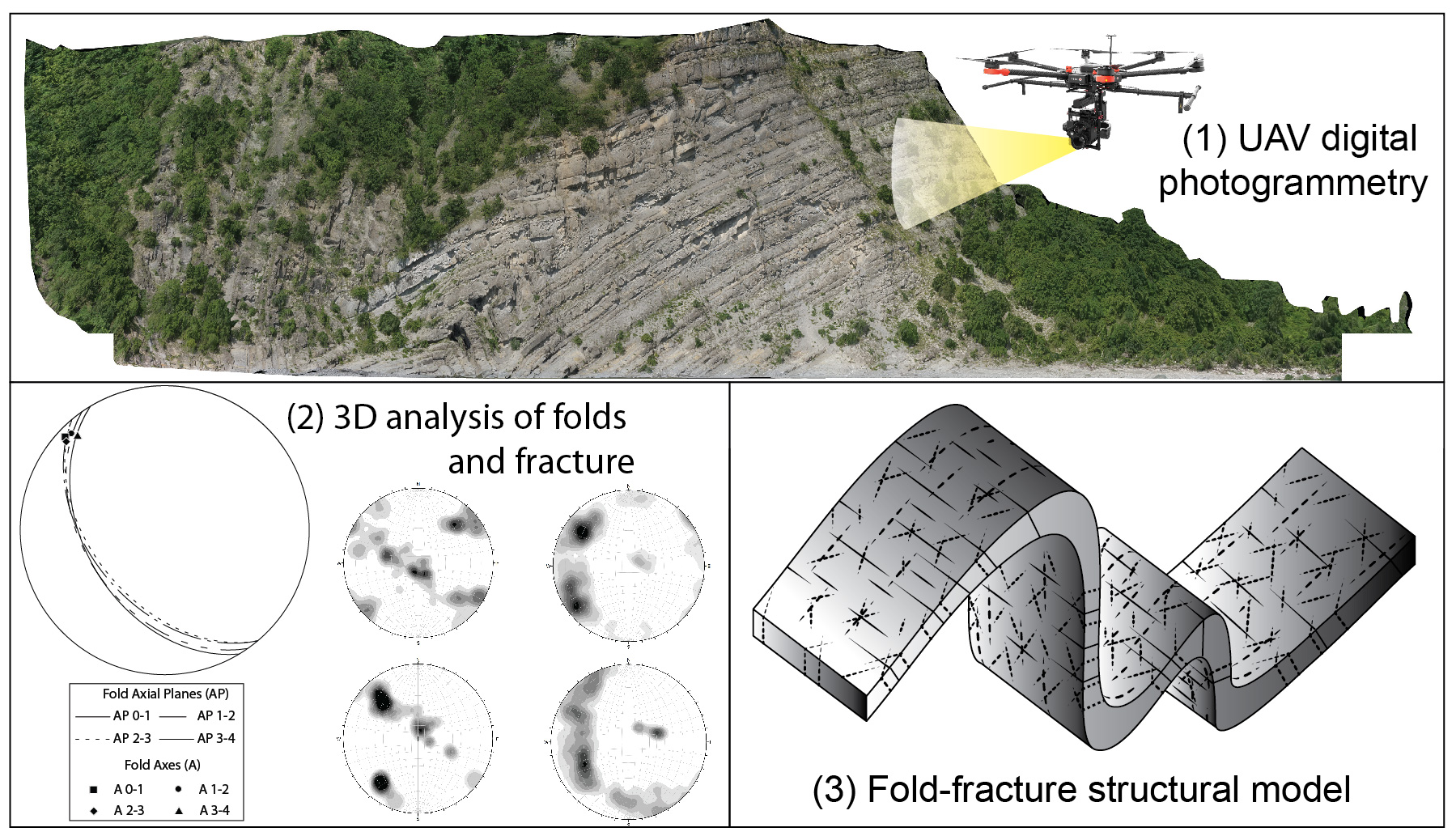
Our study aims to demonstrate how the application of UAVDP can dramatically improve the structural analysis of folded and fractured rocks by acquiring a great amount of digital data from inaccessible (partially or totally) outcrops and increasing the sampling of the deformation structures. In particular, this study demonstrates as UAVDP technique allows for analyzing the relationships between folds and fractures in a flysch formation.
In the North-Western Italian Appennines, the Ponte Organasco area offers the possibility to study the meso-scale deformations that affect Monte Antola formation (
Figure 1). In this area the erosion of the Trebbia river creates several spectacular cliffs, almost completely inaccessible by field surveys, and characterized by several folds and brittle structures.
2. Geological Setting
The study area is located in NW Apennines, near Ponte Organasco village at the confluence between Avagnone and Trebbia rivers, nearly 100 km north of Genoa (
Figure 2). In this area, the Antola Unit (AU) crops out extensively and is affected by a great number of folds, faults and fractures developed in absence of metamorphism.
From bottom to the top, the AU unit [
20,
21,
22] is composed by:
varicolored hemipelagic shales (the Late Cenomanian-Early Turonian Montoggio Shale-“Argilliti di Montoggio”) followed by thin-bedded, siliciclastic and carbonatic turbidites (Early Campanian Gorreto Sandstone—“Arenarie di Gorreto”);
carbonate turbidite (Early Campanian-Early Maastrichtian Monte Antola Formation-“Formazione di Monte Antola” or “Calcare del Monte Antola”);
siliciclastic-carbonatic turbidite (Early Maastrichtian-lower Late Maastrichtian Bruggi-Selvapiana Formation—“Formazione di Bruggi-Selvapiana” and the Late Maastrichtian-Late Paleocene Pagliaro Shale—“Argilliti di Pagliaro”).
AU is topped by the Tertiary Piedmont Basin (TPB), a wedge-top-basin located on top of the junction between the Western Alps and the Northern Apennines, that is characterized by a continuous deposition from the Mid Eocene (Monte Piano Marls) to the Late Miocene [
23].
The examined outcrops are all in the Monte Antola Formation. Locally, it is composed of dominantly turbiditic calcareous graded beds, calcareous sandstones, sandstones and marlstones, with rare intervening thin, carbonate-free graded layers or uniformly fine-grained shale. The formation is interpreted as a deep-sea basin plain deposit, with local lateral facies variations which range from proximal, thick-bedded turbidites to distal turbidites with predominantly thickening upward cycles and a high percentage of pelites. The thickness of the more competent beds varies, but on average it ranges between 1.5 and 2 m.
In the study area, the AU (locally represented by Monte Antola Formation and Montoggio Shale) overthrusts onto the “Argille a palombini di Monte Veri” Formation, belonging to the External Ligurian Unit (
Figure 2).
The collisional belt of the Northern Apennines can in fact be subdivided into three major groups of units characterized by defined structural and paleogeographic domains: (1) Tuscan Units; (2) Sub-Ligurian Units and (3) Ligurian Units [
24]. The NE sector of the Northern Apennines is mainly represented by the Ligurian Units (
Figure 1).
Ligurian Units are placed at top of the nappe pile due to the Apenninic tectonic stage (Oligocene and Miocene-Pleistocene) thrusting onto the more external domain of continental margin of Adria (Sub-Ligurian and Tuscan domain; [
20]). These units are characterized by an assemblage of ophiolitic sequences of Jurassic age and the related sedimentary successions-(Late Jurassic to Middle Eocene [
25]) and represent the transition between the Ligurian-Piedmont ocean fragments and the Adria continental margin [
22].
Elter [
24] subdivided Ligurian units into two groups according to their structural and stratigraphic features: Internal Ligurian Units (ILU) and External Ligurian Unit (ELU). The ILU derived from oceanic basin setting whereas the ELU from the transition from ocean basin to continental margin of the Adriatic plate [
25].
The ILU are thrusted onto the ELU along the Levanto-Ottone tectonic line (
Figure 1).
The AU is geometrically the highest unit outcropping in this sector of the Apenninic chain, nevertheless it has been recently ascribed to eastern ELU due to the lack of ophiolitic debris in its basal complex [
22].
The strong deformations affecting the Monte Antola Formation are difficult to investigate because of the inaccessibility of the outcrops, often represented by vertical or sub-vertical cliffs or slopes. Moreover, the ductile deformations are accompanied by well-developed fracture networks that enhance circulation of fluid causing frequent problems of slope stability.
3. Study Area
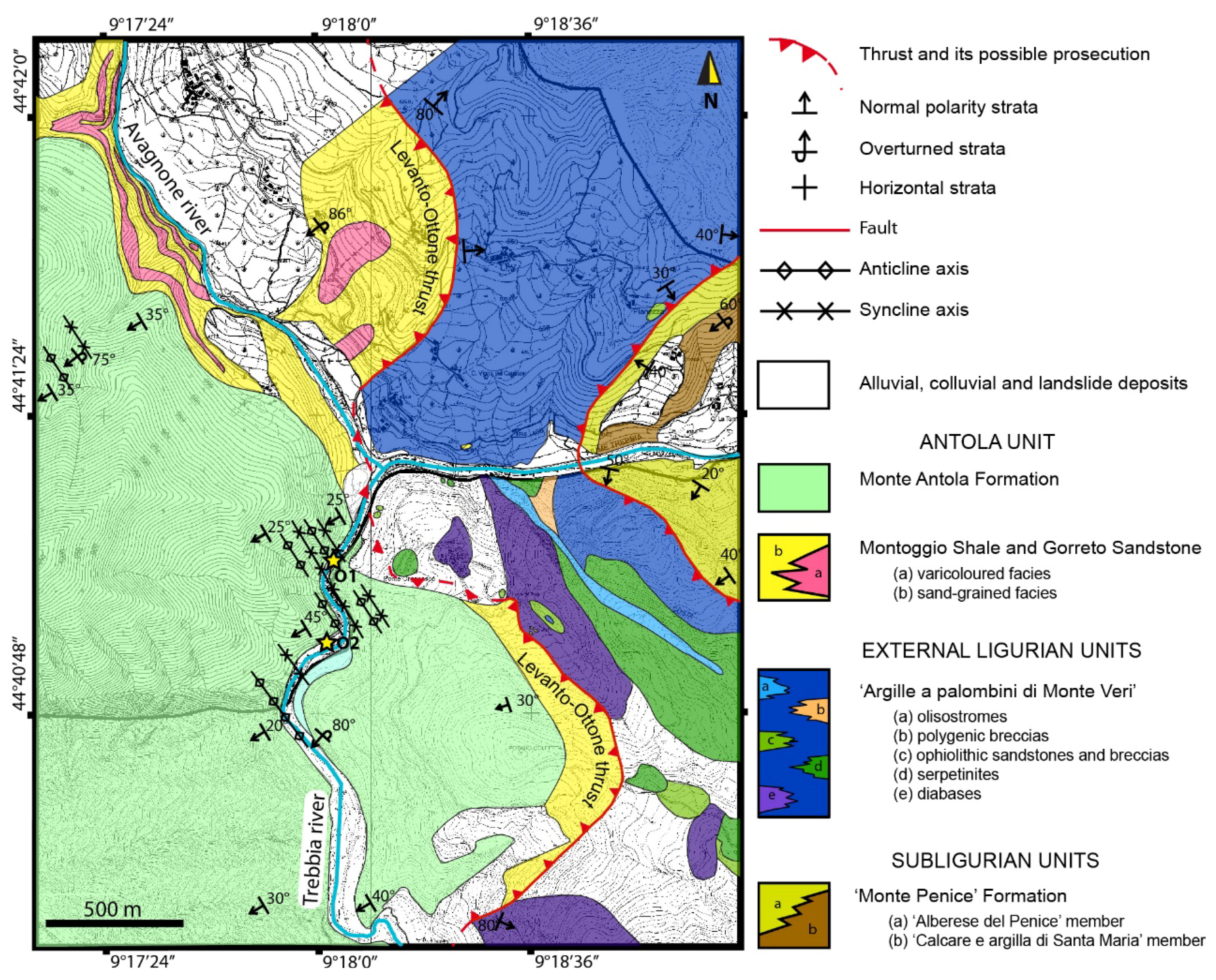
The study area is located near Ponte Organasco village (Lat. 44.685° N; Long. 9.306° E), where the AU overthrusts on the ELU locally represented by the “Argille a palombini di Monte Veri” formation, that is made up by heavily deformed dark shales interbedded with silica-rich limestones, and polygenic breccias, ophiolites and olistolites. Due to the proximity of this thrust, the Monte Antola Formation is affected by a series of thrust related folds, faults and fractures (
Figure 2).
Two outcrops of the Monte Antola Flysch, both located along Trebbia river (
Figure 3), have been studied by means of DP.
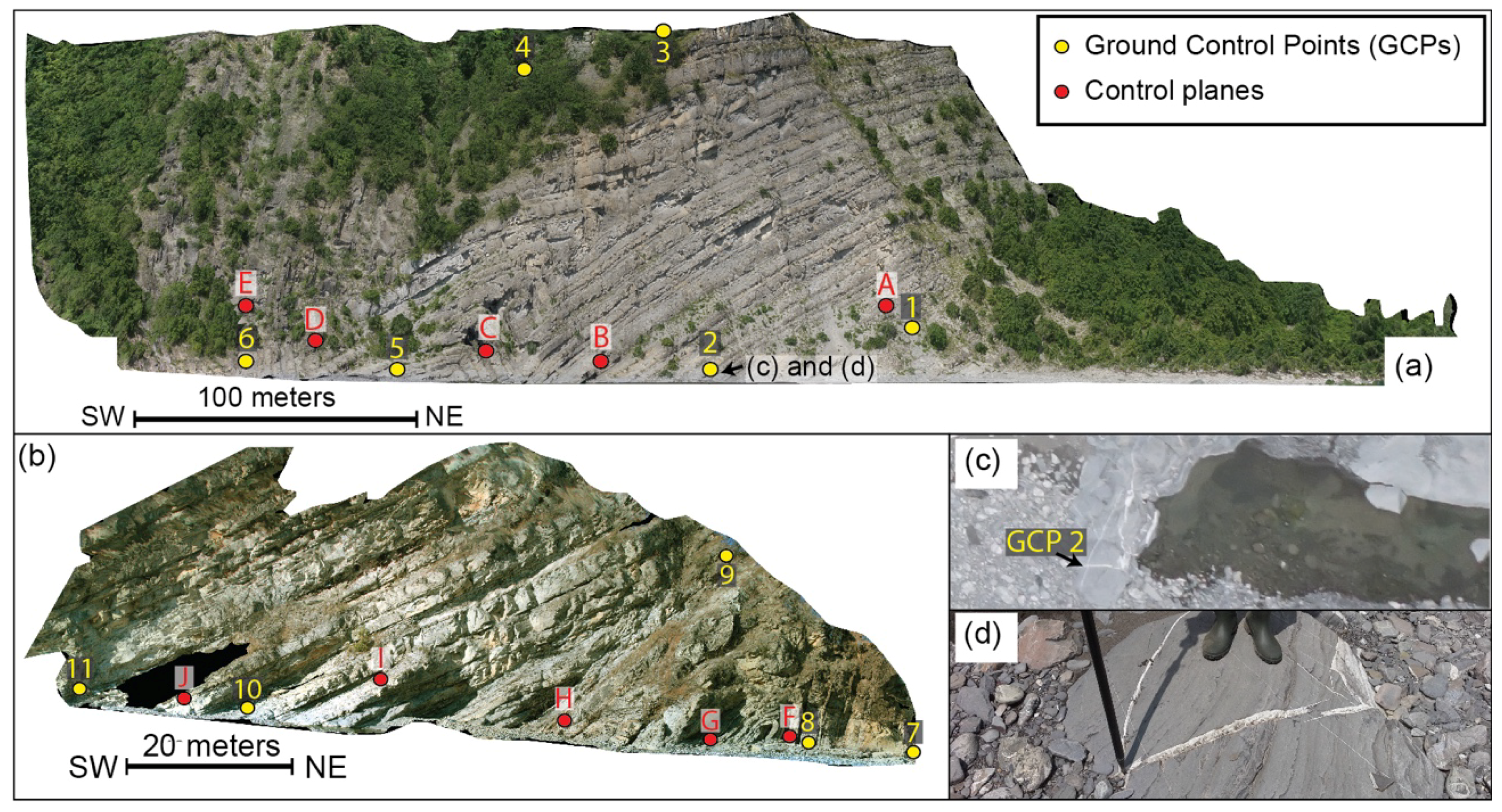
The first outcrop (O1) is a sub-vertical cliff 100 m high and more than 200 m wide, oriented SW-NE, showing well exposed folding structures (
Figure 4a). The second outcrop (O2) is a sub-vertical cliff 40 m high and 100 m wide, oriented SW-NE (
Figure 4b). These outcrops were investigated by UAVDP because of the impossibility to obtain satisfactory information by structural field surveys.
4. Methodology
4.1. UAV Digital Photogrammetry (UAVDP) Surveys
Due to the inaccessibility and huge dimension of the outcrops (sub-vertical slopes more than 50 m in height) two UAVDP surveys were conducted in order to obtain two high-resolution DOMs and to avoid TDP problems of censoring and bias induced by unfavorable orientations of the camera [
5]. A mirrorless Sony ILCE-6000 24 Megapixel camera (APS-C sensor), (Sony Europe Limited, Weybridge, UK) with 16 mm lens, was mounted on a hexacopter (UAV) using a 2-axis gimbal. Main specifications of UAV and camera are reported in
Table 1.
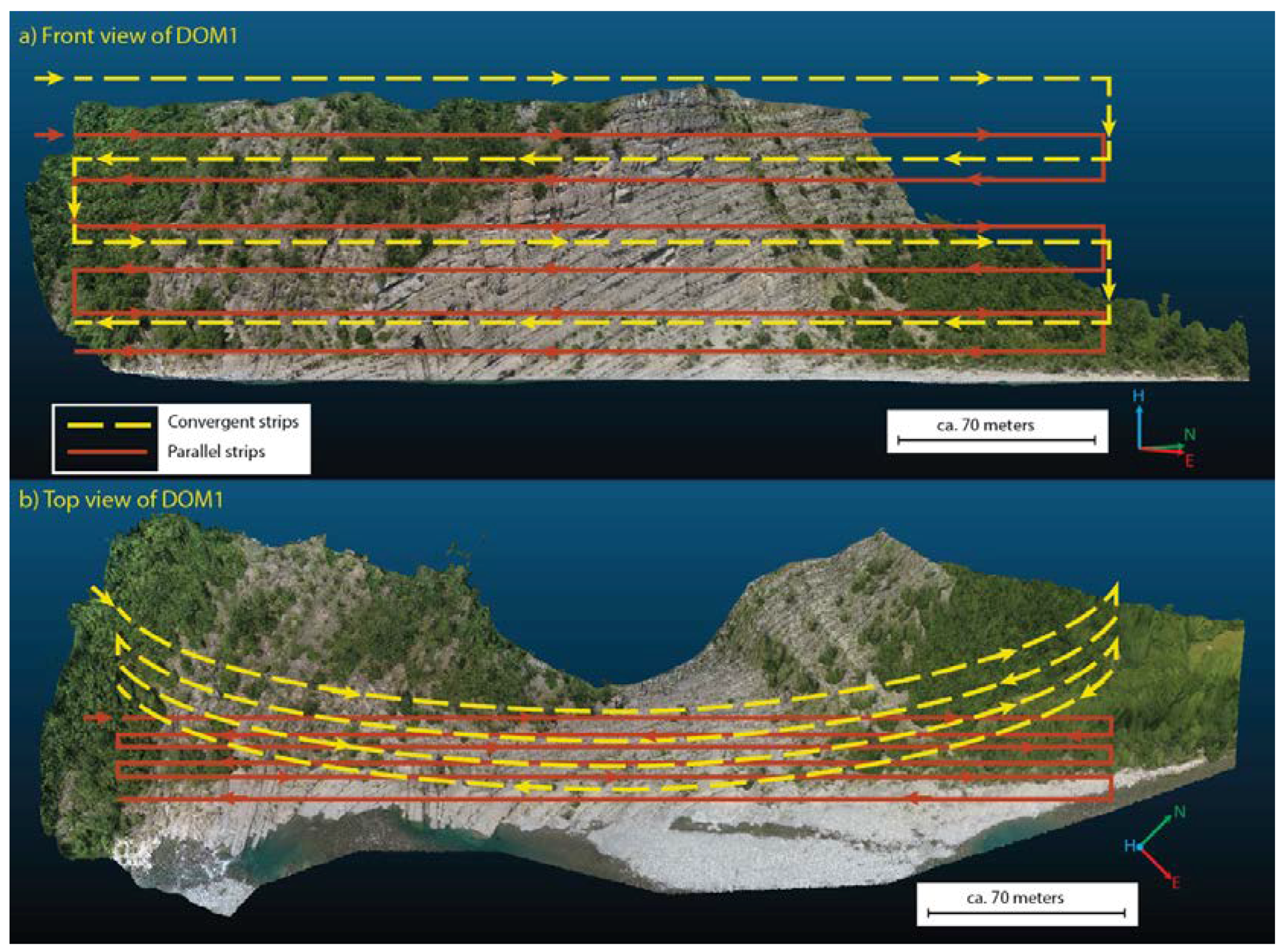
The UAVDP surveys were conducted with an oblique orientation of the on-board camera and the acquisition of digital photographs with a minimum overlap and sidelap of about 85% and 65%, respectively. In order to capture the complex geometry of the outcrops and to improve the accuracy of the generated DOMs, the images were acquired from positions parallel (strips of photographs taken along a fly line) and convergent to the outcrop [
26]. The distance from the camera to the closest rock surface was from 15 to 52 m. According to Birch [
26], giving to the camera setting and the camera-outcrop distances the Ground Sample Distances (GSDs) of the photographs are between 4 and 13 mm. The flights were flown under manual control in a sequence of back-and-forward flight lines to cover the full vertical extent of the rock outcrops (
Figure 5).
All photographs (334 for DOM1 and 145 for DOM2) were georeferenced and oriented by the UAV-on board GNSS/IMU instrumentations and 11 natural Ground Control Points (GCPs—see
Figure 3 and
Figure 4) that were acquired using a Topcon Hyper Pro Real Time Kinematic (RTK) differential GPS system, with a horizontal mean error of 1.7 cm and a vertical mean error of 3.2 cm.
4.2. Digital Outcrop Models Development and Analysis
The images were processed in two different blocks using the Structure from Motion (SfM) technique [
7,
27,
28], using the software package Agisoft Photoscan (version 1.2.5, Agisoft LLC, St. Petersburg, Russia) [
29]. The alignment of the images and the development of the sparse point clouds were conducted using 11 non-collinear GCPs (6 and 5 GCPs respectively for the two outcrops, see
Figure 3 and
Figure 4) and the full resolution of the photographs. The dense point clouds were calculated subsampling the photographs by a factor of 2 in each dimension in order to develop easy-manageable point clouds (<51 millions of points) in a reasonable time. Finally two textured meshes were created (mean surface of the triangle faces ~1 cm
2). The accuracy of the developed DOMs, will be discussed in the next paragraph. DOM1 and DOM2 are respectively referred to O1 and O2.
Table 2 and
Table 3 show the main features of the DOMs.
The DOMs were interpreted using the open-source software Cloud Compare version 2.9 [
30], that allows the stereo-vision of the models and digital sampling of bedding and fractures. The stereo-visualization and structural interpretation of the DOMs were performed by a Planar SD2220W stereoscopic monitors. Only in stereo-vision, in fact, it is possible to understand the real nature and geometry of the structures (strata, fractures, lineations, folds, etc.) and to avoid misinterpretations due to 2D visualization on standard monitors of 3D objects.
The procedure to measure the orientation of a bedding or fracture plane using Cloud Compare software consists of point-picking the intersection between the selected fracture/bedding surface and the DOM’s surface. Then the best-fit plane of the picked points is calculated. Bedding and fracture orientation were also mapped using the compass [
31] new plugin of Cloud Compare that permits to sample traces on point clouds in a semi-automatic way and to extract their position, orientation and length.
4.3. Accuracy of DOMs
The accuracy of a DOM can be distinguished in absolute and relative accuracy [
32]. Absolute accuracy refers to the difference between the reconstructed position of a point of the DOM, calculated by SfM procedure, and the location of the same point on Earth (e.g., latitude, longitude, and elevation). Relative accuracy is a measure of positional coherence between a point and the neighboring points that is the difference in length and azimuth of the vectors that join two points on Earth, and the corresponding length and azimuth of the same vectors in the model.
For geological and structural outcrop studies, relative accuracy is certainly more important because the measurements (e.g., attitudes of plane and surfaces) calculated in a DOM characterized by good relative accuracy are equivalent to measurements made on the outcrop. An accurate absolute location of these measures is often less important for geological purposes.
The influence of georeferenced UAVDP models on surface orientation measurements (e.g., beds and fractures dip and dip azimuth) are comparable to the accepted range of errors of the user/instrument orientation measurements [
33]. This range (ca. ±2°) could be defined by the accuracy of high level compass-clinometer instrument [
34] and by the statistical significance of field measurements of not perfectly planar surfaces (e.g., slightly undulated surfaces).
The absolute accuracy of the study DOMs georeferenced using 11 GCPs was calculated by comparing GCPs coordinate measured by the RTK differential GPS system and those estimated in the model (
Table 4). Their comparison shows a mean horizontal difference of 0.41 m with a standard deviation of 0.16 m and a vertical difference of 0.30 m with a standard deviation of 0.18 m.
The relative accuracy of the model was evaluated comparing:
the lengths and orientations of the vectors that join the GCPs estimated both by the GPS measurements and by the digital measurements performed on the model (
Table 5).
the attitudes of 10 control planes (5 planes on each outcrop, see
Figure 6) accurately measured in the field and in the stereo-vision of DOMs (
Table 6).
The results indicate a high degree of relative accuracy of the model, with maximum angular differences in the attitude and length of the vectors encompassed in ±2° and 0.3%, respectively. The comparison of field and DOMs measures (
Table 6) shows a maximum angular difference of ~2° for both DOM1 and DOM2. As previously outlined, these values cannot be considered errors because manual sampling could be affected by orientation bias due to the local variation of surface orientations, whereas DOM sampling could overcome orientation bias collecting the orientation that best fits the entire surface. These angular differences confirm the validity of the DOMs and their good relative accuracy. On the whole, the substantial agreement between field manual and DOM digital measures largely counterbalances the not completely satisfying absolute accuracy of the models; the latter is probably due to the few measurable GCPs that are concentrated essentially at the base of the rock slopes.
5. Results
5.1. Folds Analysis
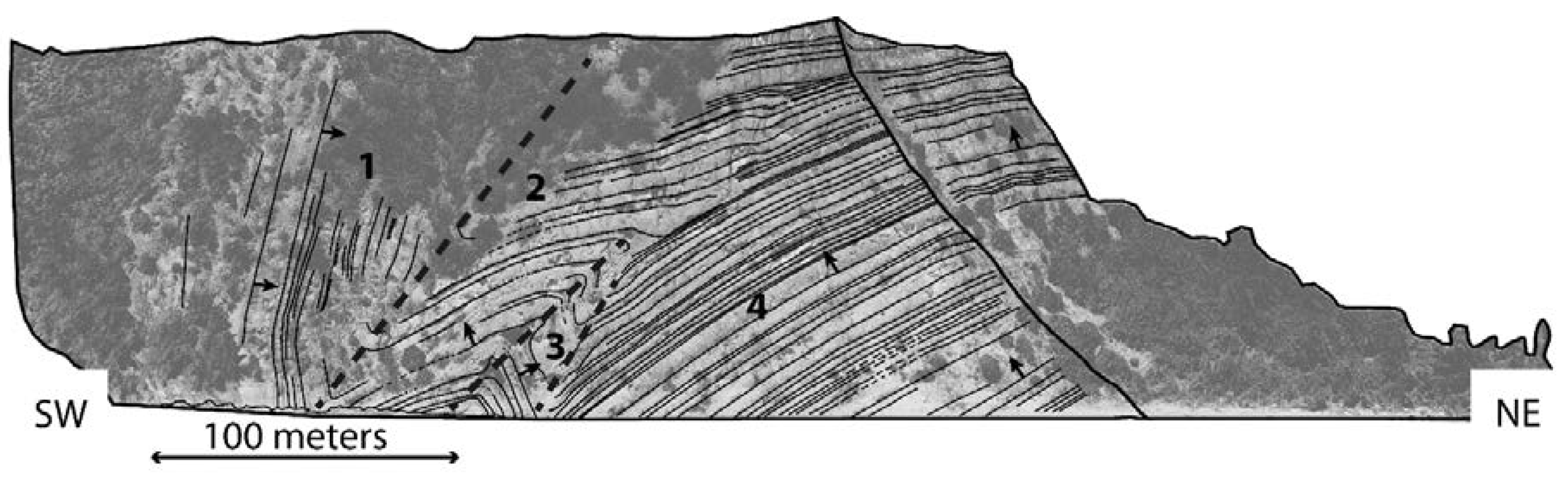
A series of NE-vergent overturned folds were identified by means of stereoscopic analysis and interpretation of textured DOMs. The DOMs were subdivided into domains corresponding to different limbs.DOM1 was subdivided into 4 main fold limb domains (
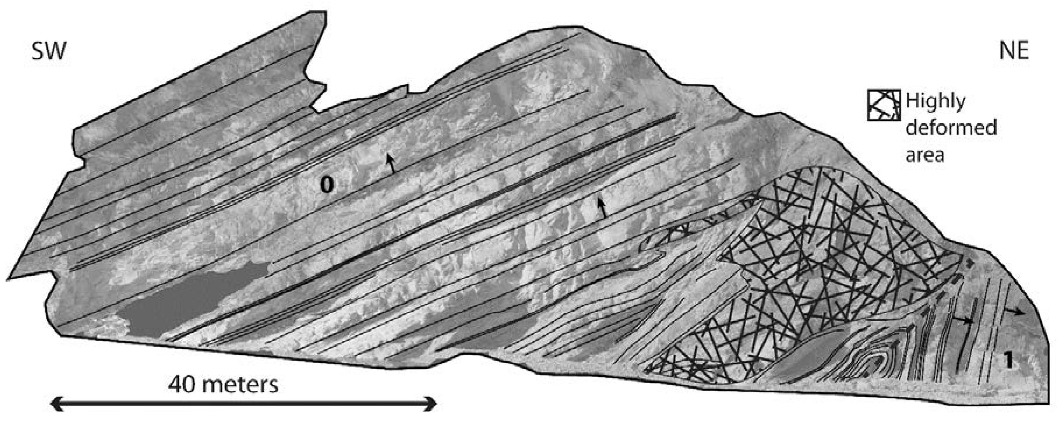
Figure 7), whereas DOM2 was subdivided into 2 main fold limb domains (
Figure 8).
In DOM1 the limb 4 (L4;
Figure 5) is formed by sub-parallel beds dipping towards SW. The surface morphology, colors and shape of the beds suggest a normal polarity of the strata. This hypothesis was confirmed by field controls. By the analysis of DOM1 29 beds of L4 were measured and their orientation statistics were calculated (see
Table 7).
The bedding has a mean attitude (dip direction and dip) of 244° N 36°. L4 and L3 form a NE-vergent overturned syncline (
Figure 7). This fold (F3-4) decreases of magnitude upward until disappears.
Only 7 bed orientations of L3 were sampled for its limited dimensions. The mean attitude of these beds is 37° N 76° (see
Table 7). L3 and the lower part of L2 form an overturned NE-vergent anticline (F2-3;
Figure 7).
A total of 22 bed orientations of L2 were sampled. The mean attitude of L2 beds is 246° N 22° (see
Table 7). L2 and L1 form a NE-vergent overturned syncline (F1-2;
Figure 7).
L1 is characterized by overturned beds with a mean attitude of 228° N 80°. Limb L1 is visible on DOM1 and DOM2 (see
Figure 7 and
Figure 8); the analysis performed on both the models allowed the acquisition of the measures of 20 beds (
Table 7).
A total of 15 bed orientations were measured also on Limb L0 that forms with limb L1 another NE-vergent overturned anticline (F0-1). Here the mean attitude of the beds is 235° N 24° (
Table 7).
The digital measurements of bedding attitude of each fold limbs (
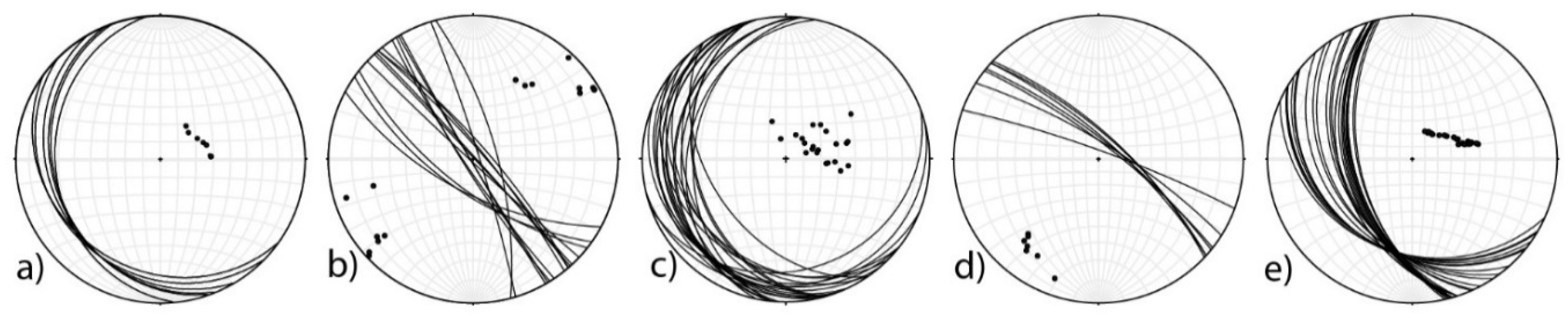
Figure 9) and their statistic parameters such as mean dip direction, dip and K-Fisher distribution coefficient (see
Table 7), allowed to calculate the orientation of fold axes and axial planes and the different interlimb angles (
Figure 10;
Table 8).
The folds show very similar features; they are endowed with sub-horizontal or slightly NW dipping axes and SW dipping axial planes, indicating that they belong to the same deformation phase.
The geometry of the investigated asymmetric folds (z-shaped looking towards NW) indicates a vergence towards NE and confirms the tectonic transport towards NE of the Antola Unit, driven by the Levanto-Ottone thrust, which is located immediately NE of the area (
Figure 1 and
Figure 2).
5.2. Fracture Analysis
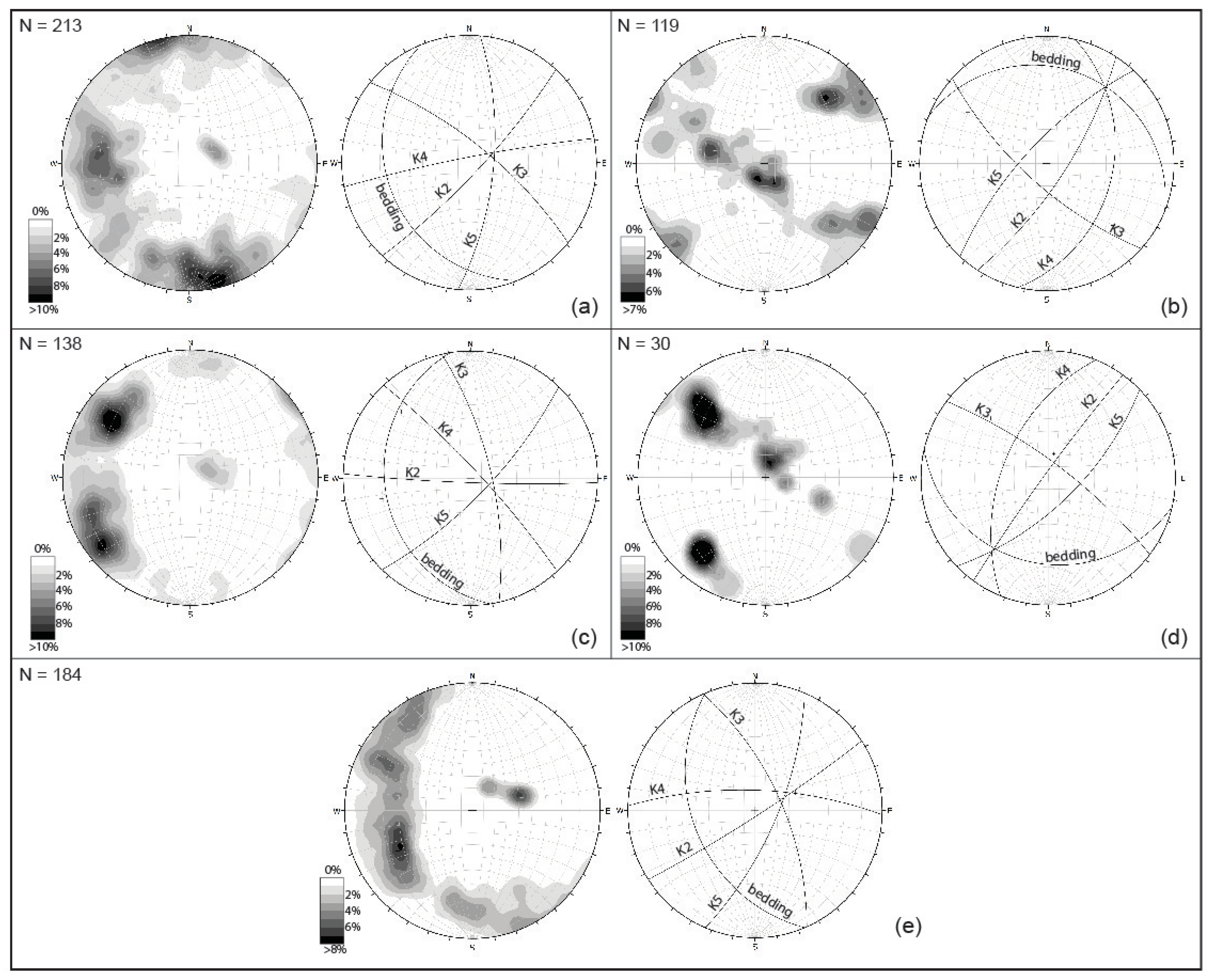
Fracture analysis was conducted on each limb of the folds visible on the two DOMs. 213, 119, 138, 30, 184 fractures were measured on limbs L0 to L4, respectively. The identified fractures can be subdivided into 4 sets (
Table 9,
Table 10,
Table 11 and
Table 12).
Fracture analysis shows that all the sets of fracture are generally strata bound and always sub-orthogonal to the bedding; besides the angular relationships among these four sets and those between this network of fractures and the bedding planes are almost the same for all the fold limbs (
Figure 11).
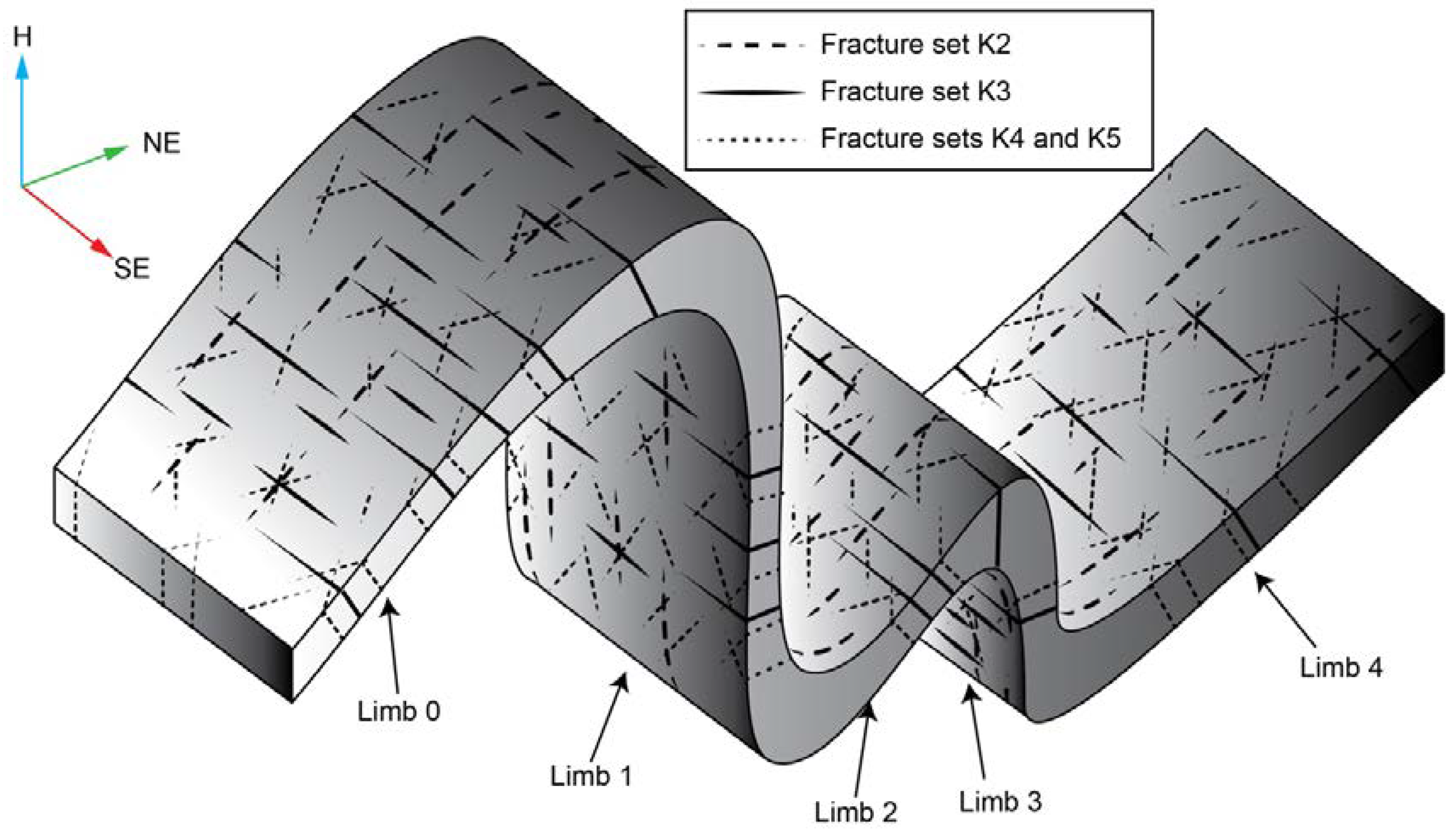
These features allow for correlating the fracture sets of the different fold limbs considering that sets K2 and K3 are sub-orthogonal and sub-parallel to the fold axes and to the directions of the bedding planes, while sets K4 and K5 are oblique. The set K3 can be interpreted as a joint set striking parallel to the fold hinge and dipping normal to bedding. It may be associated with outer-arc stretching during folding; regions of localized tensional stresses develop in the same orientation as regional compression, leading to fracture opening. The K2 joint set, which strikes perpendicular to the fold hinge and dips normal to bedding may be associated with localized extension in a direction perpendicular to the tectonic transport.
The remaining fractures associated with these thrust related folds are two sets of conjugate shear fractures (K4 and K5) generally with an acute bisector parallel to the tectonic transport direction. These fractures may form due to regional compression or localized inner-arc compression associated with tangential longitudinal strain folding (
Figure 12).
Incomplete assemblages of these fractures are seen at limb3 where only one K2-fracture is visible.
6. Concluding Remarks
Our study demonstrates that the Digital Photogrammetry (DP) techniques and in particular those based on Unmanned Aerial Vehicle (UAV) technologies can produce Digital Outcrop Models (DOMs) of high accuracy and low costs that can be successfully applied to detailed structural analysis of rock outcrops. The principal advantages of this technique are: (1) the possibility to analyze outcrops, totally or partially inaccessible; (2) obtaining a largest number of measures and data; (3) acquiring more representative measures of geological planes (strata, faults and fractures) with respect to manual sampling, because the measurements are not influenced by the local variations of attitude that typically affect the geological planes; (4) the possibility to repeat and control the analysis and the measures by different operators and at different times; (5) a substantial time savings in the phase of the fracture measurements; (6) a safe methodology especially in case of unstable and dangerous rock slope.
During this study two large inaccessible outcrops of the Monte Antola Formation, a turbiditic calcareous flysch, located in NW Apennines, near Ponte Organasco village along the Trebbia river, have been studied. From DOMs analysis, it has been possible to measure the attitude of the bedding of the whole outcrops and then calculate with good precision the orientation of fold axes and axial planes. The folds analyzed were scarcely visible and not measurable by field surveys due to the steepness (more than 80°) and height (several tens of meters) of the outcrops.
The folds are constituted by two couples of NE-vergent overturned anticlines and synclines. The folds are asymmetric (z-shaped looking towards NW), rather irregular and show major variations of thickness and shape in the hinge-regions. The interlimb angles vary from few degrees (fold between limbs 0 and 1) to about 90° (fold between limbs 3 and 2). The axes and axial planes of the folds have a similar orientation: the mean attitude of the fold axes is 319° N 5°, while the mean orientation of the axial planes is 233° N 42°.
The fold analysis indicates that the deformations affecting the Monte Antola Formation in this area have a typical Apenninic trend, with a clear NE vergence, confirming the presence and nature of the Levanto-Ottone thrust.
Similarly, the analysis of the two DOMs allowed to measure the fracture network that locally affects the flysch and to evaluate the relationships between fractures and folds, examining the whole development of the structures, from the limbs to the hinges. Also, these measurements were not achievable by field surveys for the inaccessibility of the outcrops.
All the limbs of the folds are affected by four main sets of fractures (K2, K3, K4 and K5). These sets are always sub-orthogonal to the bedding and apparently maintain the same angular relationships both among them and with the bedding in the different parts of the folds, even where the strata are sub-vertical or overturned (limb 1). This condition suggests that fractures formed in the early stages of the deformation, before the complete enucleation of the folds. In particular, considering the fractures genetically connected to the folding, set K2, that is sub-orthogonal to the fold planes, can be considered a cross/extensional/hinge-orthogonal joint set, set K3, that has a direction sub-parallel to the fold axes, can be considered a longitudinal/radial joint/hinge-parallel set, while sets K4 and K5 can be interpreted as conjugate shear fractures oblique with respect to the fold axial planes and axes, generally with an acute bisector often parallel to the thrust transport direction (
Figure 12).
Author Contributions
Performed the UAV and RTK GPS surveys and elaborate raw data, M.C. Conceptualized the study, Developed the methodology, Performed formal analysis, Prepared the initial draft, N.M. and C.P. Supervised and provided critical reviews and editing, C.M. and C.P.
Funding
This research received no external funding.
Acknowledgments
Many thanks are due to Ecates S.r.l. for the support on the fly of the UAV, to Daniel Girardeau-Montaut and other CloudCompare developers that developed the useful open-source software and continue to implement it.
Conflicts of Interest
The authors declare no conflict of interest.
References
- Powers, P.S.; Chiarle, M.; Savage, W.Z. A digital photogrammetric method for measuring horizontal surficial movements on the Slumgullion earthflow, Hinsdale County, Colorado. Comput. Geosci. 1996, 22, 651–663. [Google Scholar] [CrossRef]
- Xu, X.; Aiken, C.L.; Bhattacharya, J.P.; Corbeanu, R.M.; Nielsen, K.C.; McMechan, G.A.; Abdelsalam, M.G. Creating virtual 3-D outcrop. TLE Soc. Explor. Geophys. 2000, 19, 197–202. [Google Scholar] [CrossRef]
- Pringle, J.K.; Westerman, A.R.; Clark, J.D.; Drinkwater, N.J.; Gardiner, A.R. 3D high-resolution digital models of outcrop analogue study sites to constrain reservoir model uncertainty: An example from Alport Castles, Derbyshire, UK. Petrol. Geosci. 2004, 10, 343–352. [Google Scholar] [CrossRef]
- Bellian, J.A.; Kerans, C.; Jennette, D.C. Digital outcrop models: Applications of terrestrial scanning lidar technology in stratigraphic modeling. J. Sediment. Res. 2005, 75, 166–176. [Google Scholar] [CrossRef]
- Sturzenegger, M.; Stead, D. Close-range terrestrial digital photogrammetry and terrestrial laser scanning for discontinuity characterization on rock cuts. Eng. Geol. 2009, 106, 163–182. [Google Scholar] [CrossRef]
- Jaboyedoff, M.; Oppikofer, T.; Abellán, A.; Derron, M.H.; Loye, A.; Metzger, R.; Pedrazzini, A. Use of LIDAR in landslide investigations: A review. Nat. Hazards 2012, 61, 5–28. [Google Scholar] [CrossRef]
- Westoby, M.J.; Brasington, J.; Glasser, N.F.; Hambrey, M.J.; Reynolds, J.M. ‘Structure-from-Motion’ photogrammetry: A low-cost, effective tool for geoscience applications. Geomorphology 2012, 179, 300–314. [Google Scholar] [CrossRef]
- Humair, F.; Pedrazzini, A.; Epard, J.-L.; Froese, C.R.; Jaboyedoff, M. Structural characterization of turtle mountain anticline (Alberta, Canada) and impact on rock slope failure. Tectonophysics 2013, 605, 133–148. [Google Scholar] [CrossRef]
- Bemis, S.P.; Micklethwaite, S.; Turner, D.; James, M.R.; Akciz, S.; Thiele, S.T.; Bangash, H.A. Ground-based and UAV-based photogrammetry: A multi-scale, high-resolution mapping tool for structural geology and paleoseismology. J. Struct. Geol. 2014, 69, 163–178. [Google Scholar] [CrossRef]
- Spreafico, M.C.; Francioni, M.; Cervi, F.; Stead, D.; Bitelli, G.; Ghirotti, M.; Girelli, V.A.; Lucente, C.C.; Tini, M.A.; Borgatti, L. Back Analysis of the 2014 San Leo Landslide Using Combined Terrestrial Laser Scanning and 3D Distinct Element Modelling. Rock Mech. Rock Eng. 2016, 49, 2235–2251. [Google Scholar] [CrossRef]
- Tavani, S.; Corradetti, A.; Billi, A. High precision analysis of an embryonic extensional fault-related fold using 3D orthorectified virtual outcrops: The viewpoint importance in structural geology. J. Struct. Geol. 2016, 86, 200–210. [Google Scholar] [CrossRef]
- Remondino, F.; El-Hakim, S. Image-based 3D modelling: A review. Photogramm. Rec. 2006, 21, 269–291. [Google Scholar] [CrossRef]
- Colomina, I.; Molina, P. Unmanned aerial systems for photogrammetry and remote sensing: A review. ISPRS J. Photogramm. Remote Sens. 2014, 92, 79–97. [Google Scholar] [CrossRef]
- Niethammer, U.; James, M.R.; Rothmund, S.; Travelletti, J.; Joswig, M. UAV-based remote sensing of the Super-Sauze landslide: Evaluation and results. Eng. Geol. 2012, 128, 2–11. [Google Scholar] [CrossRef]
- Lucieer, A.; Jong, S.M.D.; Turner, D. Mapping landslide displacements using Structure from Motion (SfM) and image correlation of multi-temporal UAV photography. Prog. Phys. Geogr. 2014, 38, 97–116. [Google Scholar] [CrossRef]
- Tannant, D.D. Review of Photogrammetry-Based Techniques for Characterization and Hazard Assessment of Rock Faces. Int. J. Geohazards Environ. 2015, 1, 76–87. [Google Scholar] [CrossRef]
- Casella, E.; Rovere, A.; Pedroncini, A.; Stark, C.P.; Casella, M.; Ferrari, M.; Firpo, M. Drones as tools for monitoring beach topography changes in the Ligurian Sea (NW Mediterranean). Geo-Mar. Lett. 2016, 36, 151–163. [Google Scholar] [CrossRef]
- Salvini, R.; Mastrorocco, G.; Seddaiu, M.; Rossi, D.; Vanneschi, C. The use of an unmanned aerial vehicle for fracture mapping within a marble quarry (Carrara, Italy): Photogrammetry and discrete fracture network modelling. Geomat. Nat. Hazards Risk 2016, 8, 34–52. [Google Scholar] [CrossRef]
- Sturzenegger, M.; Stead, D.; Elmo, D. Terrestrial remote sensing-based estimation of mean trace length, trace intensity and block size/shape. Eng. Geol. 2011, 119, 96–111. [Google Scholar] [CrossRef]
- Levi, N.; Ellero, A.; Ottria, G.; Pandolfi, L. Polyorogenic deformation history recognized at very shallow structural levels: The case of the Antola Unit (Northern Apennine, Italy). J. Struct. Geol. 2006, 28, 1694–1709. [Google Scholar] [CrossRef]
- Catanzariti, R.; Ellero, A.; Levi, N.; Ottria, G.; Pandolfi, L. Calcareous nannofossil biostratigraphy of the Antola Unit succession (Northern Apennines, Italy): New age constraints for the Late Cretaceous Helminthoid Flysch. Cretaceous Res. 2007, 28, 841–860. [Google Scholar] [CrossRef]
- Marroni, M.; Meneghini, F.; Pandolfi, L. Anatomy of the Ligure-Piemontese subduction system: Evidence from Late Cretaceous–middle Eocene convergent margin deposits in the Northern Apennines, Italy. Int. Geol. Rev. 2010, 52, 1160–1192. [Google Scholar] [CrossRef]
- Cavanna, F.; Di Giulio, A.; Galbiati, B.; Mosna, S.; Perotti, C.R.; Pieri, M. Carta geologica dell’estremità orientale del Bacino Terziario Ligure-Piemontese. Atti Ticinensi di Scienze della Terra 1989, 32, 191–195. (In Italian) [Google Scholar]
- Elter, P. L’ensemble Ligure. Available online: http://www.beactiveliguria.it/fr/beactive-fr/%C3%A0-pieds.html (accessed on 8 August 2018).
- Marroni, M.; Molli, G.; Montanini, A.; Ottria, G.; Pandolfi, L.; Tribuzio, R. The External Liguride units (Northern Apennine, Italy): From rifting to convergence history of a fossil ocean–continent transition zone. Ofioliti 2002, 27, 119–132. [Google Scholar]
- Birch, J.S. Using 3DM Analyst mine mapping suite for rock face characterization. In Proceedings of the 41st U.S. Rock Mechanics Symposyum: Laser and Photogrammetric Methods for Rock Face Characterization, Asheville, NC, USA, 28 June–1 July 2009; pp. 13–32. [Google Scholar]
- Spetsakis, M.; Aloimonos, J.Y. A multi-frame approach to visual motion perception. Int. J. Comput. Vis. 1991, 6, 245–255. [Google Scholar] [CrossRef]
- Boufama, B.; Mohr, R.; Veillon, F. Euclidean constraints for uncalibrated reconstruction. In Proceedings of the Fourth International Conference on Computer Vision, Berlin, German, 11–14 May 1993; pp. 466–470. [Google Scholar]
- Agisoft Photoscan (Version 1.2.5). Available online: http://www.agisoft.com/ (accessed on 7 August 2018).
- CloudCompare (Version 2.9). Available online: http://www.danielgm.net/cc/ (accessed on 7 August 2018).
- Thiele, S.T.; Grose, L.; Samsu, A.; Micklethwaite, S.; Vollgger, S.A.; Cruden, A.R. Rapid, semi-automatic fracture and contact mapping for point clouds, images and geophysical data. Solid Earth 2017, 8, 1241–1253. [Google Scholar] [CrossRef]
- Chesley, J.T.; Leier, A.L.; White, S.; Torres, R. Using Unmanned Aerial Vehicles and Structure-From-Motion Photogrammetry to Characterize Sedimentary Outcrops: An Example from the Morrison Formation, Utah, USA. Sediment. Geol. 2017, 354, 1–8. [Google Scholar] [CrossRef]
- Cawood, A.J.; Bond, C.E.; Howell, J.A.; Butler, R.W.; Totake, Y. LiDAR, UAV or compass-clinometer? Accuracy, coverage and the effects on structural models. J. Struct. Geol. 2017, 98, 67–82. [Google Scholar] [CrossRef]
- Jordá Bordehore, L.; Riquelme, A.; Cano, M.; Tomás, R. Comparing manual and remote sensing field discontinuity collection used in kinematic stability assessment of failed rock slopes. Int. J. Rock Mech. Min. Sci. 2017, 97, 24–32. [Google Scholar] [CrossRef]
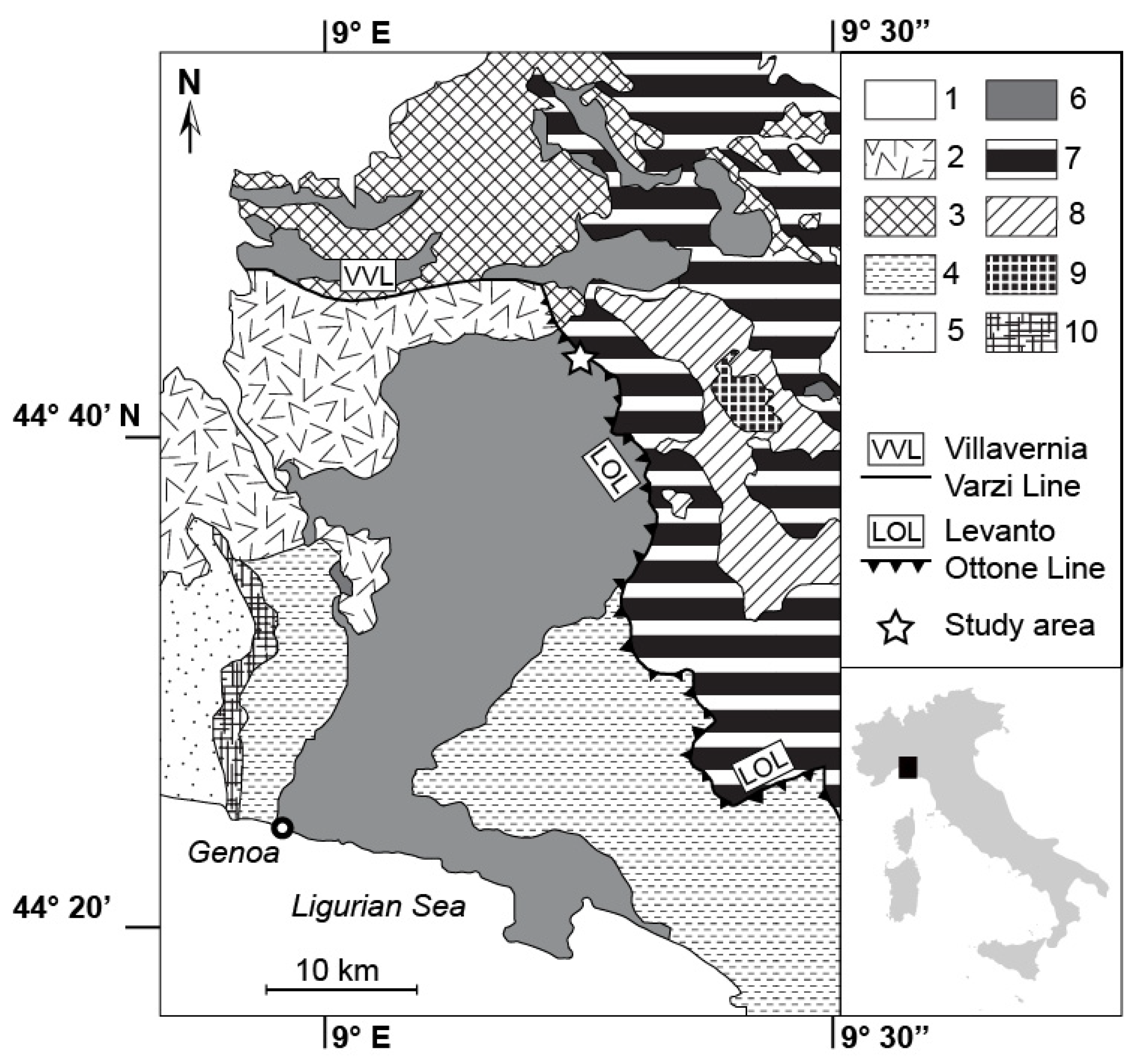
Figure 1.
Tectonic sketch of North-Western Apennines: 1: Quaternary Deposits; 2: Tertiary Piedmont Basin deposits; 3: Epiligurian Succession; 4: Internal Ligurian Units; 5: Voltri Group; 6: Antola Unit; 7: External Ligurian Units; 8: Subligurian Units; 9: Tuscan Units (Tuscan Nappe); 10: Sestri-Voltaggio Zone.
Figure 2.
Geological map of the study area.
Figure 2.
Geological map of the study area.
Figure 3.
The study outcrops marked on (a) an orthorectified aerial image and (b) a perspective image. In (b) the positions of the Ground Control Points (GCPs) are shown.
Figure 3.
The study outcrops marked on (a) an orthorectified aerial image and (b) a perspective image. In (b) the positions of the Ground Control Points (GCPs) are shown.
Figure 4.
Orthorectified images of Digital Outcrop Models DOMs representing outcrops 1 (a) and 2 (b). The view points of the orthorectified images are horizontal and sub-orthogonal to the mean slope direction. The position of the GCPs and the control planes (natural surfaces whose attitude was measured in the field and on the DOMs) are indicated with yellow and red dots, respectively. The position of GCP 2 is shown in a Unmanned Aerial Vehicle (UAV) (c) and field (d) images.
Figure 5.
(a) Front and (b) top views of the flight plan showing flight lines and direction of flight used for the photogrammetric acquisition of DOM1. Pictures were acquired from positions parallel (red lines) and convergent (yellow lines) to the outcrop. The second UAV survey conducted with the same flight scheme.
Figure 6.
(a) Textured digital outcrop model (TDOM), (b) triangular mesh and (c) field survey picture of the same portion of the outcrop 1 (peoples for scale). In (a,c) the surface representing the control plane ‘C’ are shaded in purple. In (b) the best-fit plane calculated using Cloud Compare are represented by a purple rectangle.
Figure 7.
Structural interpretation of DOM 1 (see
Figure 4a) projected on an orthorectified image. The view point of the orthorectified image is horizontal and sub-orthogonal to the mean slope direction. Beds (thin black lines) and the main traces of the fold axial planes (grey dashed lines) are shown. The numbers mark the 4 main fold limbs recognized by the preliminary visual analysis. Small black arrows show the polarity of the beds.
Figure 8.
Structural interpretation of DOM 2 (see
Figure 4b) projected on a orthorectified image. The view point of the orthorectified image is horizontal and sub-orthogonal to the mean slope direction. Beds (thin black lines) and the main trace of the fold axial plane (grey dashed line) are shown. The numbers mark the 2 main fold limbs recognized by the preliminary visual analysis. Small black arrows show the polarity of the beds.
Figure 9.
Lower hemisphere stereographic projections of bedding planes and poles of limb 0 (a), limb 1 (b), limb 2 (c), limb 3 (d) and limb 4 (e).
Figure 9.
Lower hemisphere stereographic projections of bedding planes and poles of limb 0 (a), limb 1 (b), limb 2 (c), limb 3 (d) and limb 4 (e).
Figure 10.
Lower hemisphere stereographic projections of fold axial planes (AP) and fold axes (A). Folds are indicated by the connected limbs (e.g., Fold 0-1 means fold forms by limbs 0 and 1). Attitude data are shown in
Table 8.
Figure 10.
Lower hemisphere stereographic projections of fold axial planes (AP) and fold axes (A). Folds are indicated by the connected limbs (e.g., Fold 0-1 means fold forms by limbs 0 and 1). Attitude data are shown in
Table 8.
Figure 11.
Contour plot of poles (equal area, lower hemisphere, per 1% area) and cyclographic projection of the mean planes (equal angle, lower hemisphere) of bedding and fractures of limbs 0 (a), 1 (b), 2 (c), 3 (d) and 4 (e).
Figure 11.
Contour plot of poles (equal area, lower hemisphere, per 1% area) and cyclographic projection of the mean planes (equal angle, lower hemisphere) of bedding and fractures of limbs 0 (a), 1 (b), 2 (c), 3 (d) and 4 (e).
Figure 12.
A 3D interpretation of the geometrical relationships between fracture sets and folds (not to scale).
Figure 12.
A 3D interpretation of the geometrical relationships between fracture sets and folds (not to scale).
Table 1.
UAV and UAV-camera specifications.
Table 1.
UAV and UAV-camera specifications.
| UAV Type | Diameter | Engines | Rotor Diameter | Empty Weight | UAV-Camera Weight |
| hexacopter | 115 cm | brushless | 15 inch (38.1 cm) | 6.9 kg | 8.3 kg |
| Camera | Sensor Type | Sensor Size | Image Size | Pixel Size | Focal Length |
| Sony 6000 ILCE | APS-C | 23.5 × 15.6 mm | 6000 × 4000 pixels | 3.92 × 3.90 µm | 16 mm |
Table 2.
Characteristics of DOM1.
Table 2.
Characteristics of DOM1.
| Number of Images | 334 |
| Surface of the Model (m2) | 4513 |
| Distance Camera-Outcrop Range (m) | 31–52 |
| Mean Distance Camera-Outcrop (m) | 39 |
| Mean GSD at the Outcrop Surface (mm) | 9.5 |
| Number of Dense Cloud Points | ~50.5 million |
| Number of Triangular Facets | ~10.5 million |
Table 3.
Characteristics of DOM2.
Table 3.
Characteristics of DOM2.
| Number of Images. | 145 |
| Surface of the Model (m2) | 224 |
| Distance Camera-Outcrop Range (m) | 15–20 |
| Mean Distance Camera-Outcrop (m) | 3.9 |
| Mean GSD at the Outcrop Surface (mm) | 47 |
| Number of Dense Cloud Points | ~31 million |
| Number of Triangular Facets | ~3 million |
Table 4.
Absolute accuracy (GCPs errors) of DOMs in meters.
Table 4.
Absolute accuracy (GCPs errors) of DOMs in meters.
| GCPs and CKPs | Horizontal Error | Vertical Error | Total Error |
|---|
| 1 (GCP) | 0.243 | 0.203 | 0.316 |
| 2 (CKP) | 0.519 | 0.523 | 0.737 |
| 3 (GCP) | 0.357 | 0.224 | 0.421 |
| 4 (GCP) | 0.389 | 0.113 | 0.405 |
| 5 (CKP) | 0.639 | 0.274 | 0.695 |
| 6 (GCP) | 0.190 | 0.209 | 0.282 |
| 7 (GCP) | 0.369 | 0.272 | 0.458 |
| 8 (CKP) | 0.412 | 0.253 | 0.483 |
| 9 (GCP) | 0.112 | 0.048 | 0.122 |
| 10 (CKP) | 0.291 | 0.234 | 0.373 |
| 11 (GCP) | 0.351 | 0.376 | 0.515 |
| DOM1 Mean Error | 0.389 | 0.258 | 0.476 |
| DOM2 Mean Error | 0.307 | 0.237 | 0.390 |
| GCPs Mean Error | 0.287 | 0.206 | 0.360 |
| CKPs Mean Error | 0.465 | 0.321 | 0.572 |
Table 5.
Relative accuracy of attitude and length measurements of DOM1 and DOM2.
Table 5.
Relative accuracy of attitude and length measurements of DOM1 and DOM2.
| DOM | Number of GCPs Couples | Azimuth Difference | Plunge Difference | Length Difference |
|---|
| Mean | St. Dev. | Mean | St. Dev. | Mean | St. Dev. |
|---|
| 1 | 15 | 0.8° | 1.3° | 0.9° | 1.1° | 0.3% | 0.1% |
| 2 | 10 | 0.4° | 0.5° | 0.6° | 0.3° | 0.2% | 0.3% |
Table 6.
Comparison between field manual attitude measures (O1 and O2) and DOM digital attitude measures (DOM1 and DOM2). The angular difference represents the solid angle between the attitude vectors.
Table 6.
Comparison between field manual attitude measures (O1 and O2) and DOM digital attitude measures (DOM1 and DOM2). The angular difference represents the solid angle between the attitude vectors.
| Surface Label | O1 | DOM1 (UAVDP) | Angular Difference | Surface Label | O2 | DOM2 (TDP) | Angular Difference |
|---|
| A (fracture) 1 | 045° N 87° | 046° N 86° | 1° | F (bed) 2 | 227° N 80° | 227° N 78° | 2° |
| B (fracture) 1 | 130° N 43° | 129° N 45° | 2° | G (bed) 2 | 238° N 39° | 237° N 40° | 1° |
| C (bed) 1 | 046° N 86° | 046° N 84° | 2° | H (bed) 2 | 257° N 47° | 255° N 46° | 2° |
| D (bed) 1 | 318° N 84° | 318° N 82° | 2° | I (bed) 2 | 239° N 26° | 239° N 26° | 0° |
| E (bed) 1 | 225° N 85° | 226° N 85° | 1° | J (bed) 2 | 234° N 22° | 235° N 22° | 1° |
Table 7.
Fold limb mean attitude (dip direction and dip) and K-Fisher dispersion coefficient.
Table 7.
Fold limb mean attitude (dip direction and dip) and K-Fisher dispersion coefficient.
| Fold Limb Denomination | L0 | L1 1 | L2 | L3 | L4 |
| N° of Measured Beds | 15 | 20 1 | 22 | 7 | 29 |
| Mean Attitude | 235° N 24° | 228° N 80° | 246° N 22° | 037° N 76° | 244° N 36° |
| K-Fisher Coefficient | 11.79 | 19.72 | 29.65 | 82.36 | 27.61 |
Table 8.
Calculated attitudes of Axes (A) and Axial Planes (AP) and interlimb angles of the examined folds.
Table 8.
Calculated attitudes of Axes (A) and Axial Planes (AP) and interlimb angles of the examined folds.
| Fold Denomination | F0-1 | F1-2 | F2-3 | F3-4 |
| AP Attitude (Dip Direction and Dip) | 230° N 47° | 233° N 34° | 230° N 49° | 239° N 44° |
| A Azimuth [°] | 313 | 328 | 312 | 317 |
| A Plunge [°] | 6 | 0 | 9 | 12 |
| Interlimb Angle [°] | 56 | 59 | 96 | 108 |
Table 9.
Features of fracture set K2 determined in the different fold limbs.
Table 9.
Features of fracture set K2 determined in the different fold limbs.
| Fold Limb Denomination | Number of Fractures | Mean Attitude (Dip Direction and Dip) | K-Fisher Coefficient |
|---|
| L0 | 13 | 133° N 80° | 43.22 |
| L1 | 12 | 123° N 73° | 41.21 |
| L2 | 10 | 182° N 86° | 41.95 |
| L3 | 1 | 306° N 86° | - |
| L4 | 32 | 147° N 85° | 45.93 |
Table 10.
Features of fracture set K3 determined in the different fold limbs.
Table 10.
Features of fracture set K3 determined in the different fold limbs.
| Fold Limb Denomination | Number of Fractures | Mean Attitude(Dip Direction and Dip) | K-Fisher Coefficient |
|---|
| L0 | 27 | 039° N 73° | 31.04 |
| L1 | 16 | 022° N 16° | 94.70 |
| L2 | 31 | 077° N 71° | 43.67 |
| L3 | 12 | 193° N 22° | 25.91 |
| L4 | 23 | 066° N 66° | 58.76 |
Table 11.
Features of fracture set K4 determined in the different fold limbs.
Table 11.
Features of fracture set K4 determined in the different fold limbs.
| Fold Limb Denomination | Number of Fractures | Mean Attitude(Dip Direction and Dip) | K-Fisher Coefficient |
|---|
| L0 | 55 | 349° N 85° | 308.7 |
| L1 | 20 | 103° N 35° | 52.58 |
| L2 | 34 | 047° N 82° | 68.76 |
| L3 | 2 | 292° N 50° | - |
| L4 | 24 | 002° N 72° | 42.57 |
Table 12.
Features of fracture set K5 determined in the different fold limbs.
Table 12.
Features of fracture set K5 determined in the different fold limbs.
| Fold Limb Denomination | Number of Fractures | Mean Attitude(Dip Direction and Dip) | K-Fisher Coefficient |
|---|
| L0 | 46 | 095° N 68° | 37.54 |
| L1 | 19 | 313° N 71° | 39.15 |
| L2 | 50 | 134° N 74° | 51.85 |
| L3 | 13 | 136° N 66° | 47.59 |
| L4 | 42 | 113° N 70° | 37.44 |
© 2018 by the authors. Licensee MDPI, Basel, Switzerland. This article is an open access article distributed under the terms and conditions of the Creative Commons Attribution (CC BY) license (http://creativecommons.org/licenses/by/4.0/).


