Flood Risk Mapping Using GIS and Multi-Criteria Analysis: A Greater Toronto Area Case Study

Abstract

Given the increase in flood events in recent years, accurate flood risk assessment is an important component of flood mitigation in urban areas. This research aims to develop updated and accurate flood risk maps in the Don River Watershed within the Great Toronto Area (GTA). The risk maps use geographical information systems (GIS) and multi-criteria analysis along with the application of Analytical Hierarchy Process methods to define and quantify the optimal selection of weights for the criteria that contribute to flood risk. The flood hazard maps were generated for four scenarios, each with different criteria (S1, S2, S3, and S4). The base case scenario (S1) is the most accurate, since it takes into account the floodplain map developed by the Toronto and Region Conservation Authority. It also considers distance to streams (DS), height above nearest drainage (HAND), slope (S), and the Curve Number (CN). S2 only considers DS, HAND, and CN, whereas S3 considers effective precipitation (EP), DS, HAND, and S. Lastly, S4 considers total precipitation (TP), DS, HAND, S, and CN. In addition to the flood hazard, the social and economic vulnerability was included to determine the total flood vulnerability in the watershed under three scenarios; the first one giving a higher importance to the social vulnerability, the second one giving equal importance to both social and economic vulnerability, and the third one giving more importance to the economic vulnerability. The results for each of the four flood scenarios show that the flood risk generated for S2 is the most similar to the base case (S1), followed by S3 and S4. The inclusion of social and economic vulnerability highlights the impacts of floods that are typically ignored in practice. It will allow watershed managers to make more informed decisions for flood mitigation and protection. The most important outcome of this research is that by only using the digital elevation model, the census data, the streams, land use, and soil type layers, it is possible to obtain a reliable flood risk map (S2) using a simplified method as compared to more complex flood risk methods that use hydraulic and hydrological models to generate flood hazard maps (as was the case for S1).

1. Introduction

River floods represent the most frequent and expensive natural disaster affecting most of the countries around the world [1]. They take place when the river exceeds its storage capacity and the water excess overflows the banks and fills the adjacent low-lying lands, producing significant social, economic, and environmental impacts [2], including: loss of human life and negative effects on population, damage to the infrastructure and essential services, damage to crops and animals, spread of diseases, and contamination of the water supply.

Many factors contribute to river floods: heavy rains at river sources, ice jams, the melting of snow pack, and land-use change (such as deforestation and urbanization) are some important factors. Runoff after heavy precipitation is the principal reason for river floods, and as urbanization increases, impervious areas increase as well, leading to higher rates of runoff. Saturated soils, high suspended matter, and landslides also increase the negative impacts of floods.

Predicting river flood extents is a crucial aspect of flood risk management. There are three typical approaches for flood prediction: (i) analyzing the frequency of flooding, through statistical analyses, allows determining the recurrence interval for any year and for a given discharge in the stream (without explicitly characterizing the flood area); (ii) monitoring the progress of storms (e.g., amount of rainfall) can be used to predict short-term flood events; and (iii) the flood hazard maps allow determining the extent of flooded areas based on the estimated discharges for different return periods [3,4,5]. However, the flood hazard itself only assesses the extent and water depth of a flood; it does not assess the consequences on the population, economy, and environment, as flood risk assessment does. In general, risk refers to the expected losses (in terms of fatalities, or in economic terms as damage to property) of a specific hazard (in this case, flood depth and extent) to a specific element (e.g., a building in the flood hazard area) at risk in a particular future time period or future scenarios [6,7]. In this sense, flood risk assessment is the cornerstone of flood mitigation measures, as it helps decision makers and managers take action (by implementing flood prevention or mitigation strategies) to protect the exposed population or assets. Nevertheless, current flood risk management has a higher focus on assessing the damage to assets (economic loses) than the social and environmental damages [8].

1.1. GIS-Based Multi-Criteria Approach

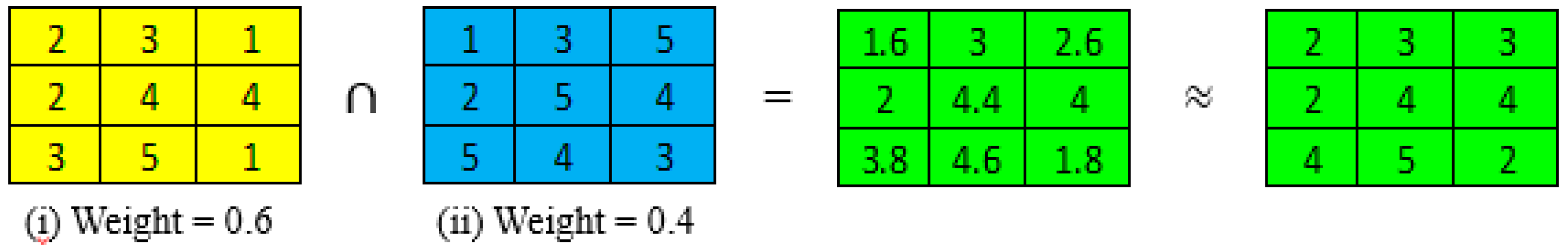
The combination of multi-criteria decision making (MCDM) with geographical information systems (GIS) proposed in the present research allows integrating the three components of risk assessment (hazard, exposure, and vulnerability), in which the social, economic, and/or environmental vulnerabilities can be considered. The outcome of this methodology is a flood risk map showing the spatial distribution of flood risk along with its intensity level, ranging from very high to very low risk. In MCDM, there are different methods for assessing criterion weights: entropy, ranking, rating, trade-off analysis, and pairwise comparison, among others [9]. The Analytic Hierarchy Process (AHP) proposed by Saaty [10] is one of the most common MCDM methods, and it has been widely applied to solve decision-making problems related to water resources [11]. The purpose of AHP is providing decision makers with the decision, among different alternatives and criteria, that best suits their goal [11,12]. This method compares two criteria at a time through a pairwise comparison matrix, in which values of relative importance from one criterion over another criterion are assigned. It provides a measure of a level of consistent judgment supported by a theoretical background. The scale of relative importance ranges between one and nine, where one is equal importance, and nine is extreme importance.

This GIS-based multi-criteria approach has been increasingly used for flood risk assessment, as it presents several advantages. Some more complex alternative methods involve hydraulic and hydrological models for flood hazard assessment, and require information of the monetary value of the assets exposed to evaluate the vulnerability [13]. In contrast, the proposed approach only requires the spatial layers of the parameters (examples of which are listed below) that contribute to the flood hazard, and land-use and demographic information to evaluate the vulnerability. Therefore, the main advantage of this methodology is the possibility of obtaining a reliable flood risk map with a relatively low monetary and time investment to support stakeholders to evaluate only the areas that need further detailed assessment. Additionally, it is easy to update, uses easy-to-get open source input data, and is flexible in terms of which criteria are included.

1.2. History of Floods in the Greater Toronto Area

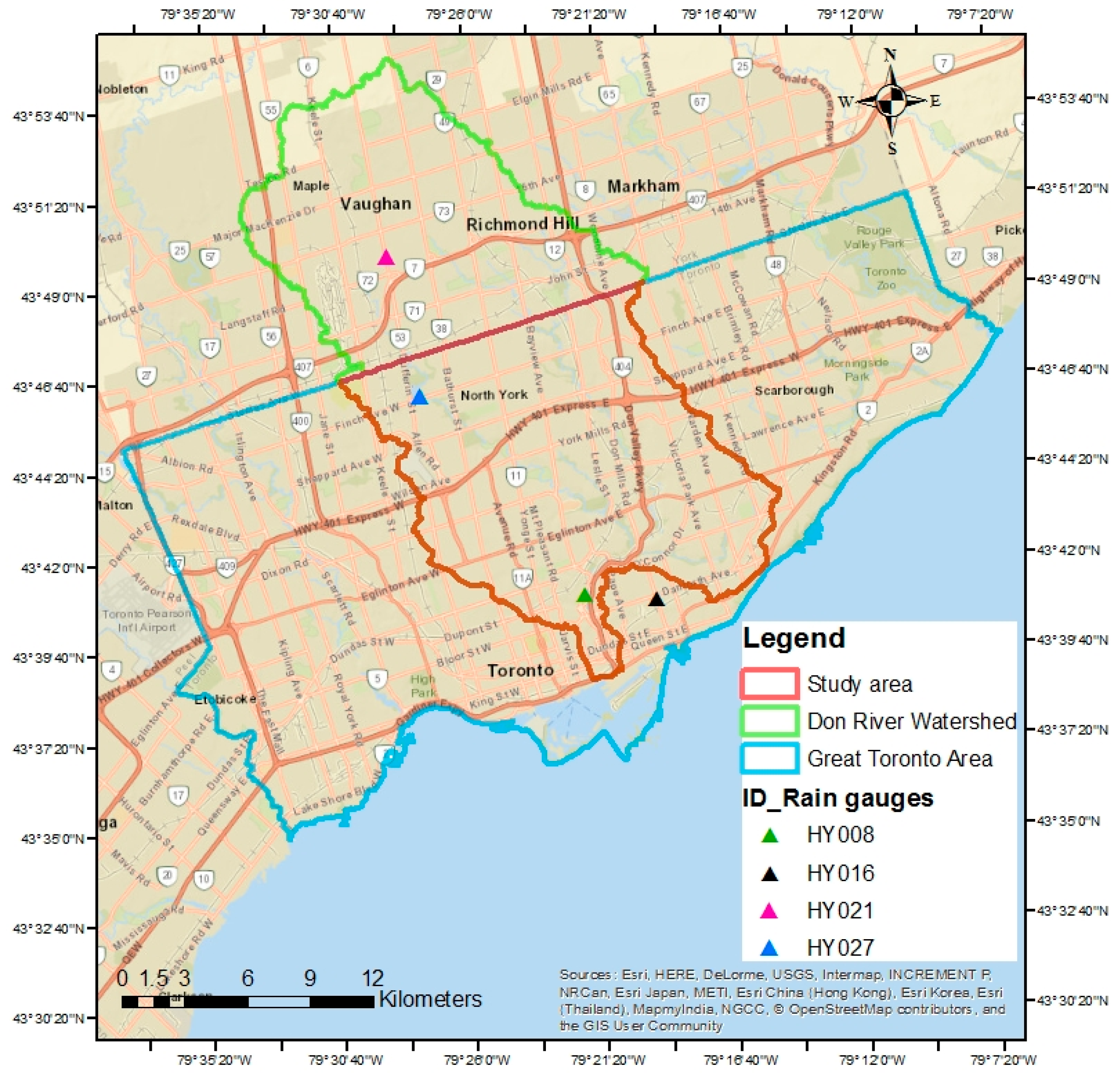
The Great Toronto Area (GTA) is selected as the case study to apply and test the proposed method. It is located in the Don River watershed in Ontario, Canada (see Figure 1 below). This region has suffered four severe flood events during the last 100 years, each of which has resulted in high economic and social impacts. Hurricane Hazel in 1945 left 81 people dead and also resulted in 1.2 billion dollars (in 2016 dollars) in damages [14]. The latest flood event, in 2013, was caused by a heavy storm in which the intensity of precipitation was 90 mm in 2 h, and some gauges reported up to 126 mm in 90 min (compared to an average of 70 mm per month [15]). There are many factors that make the GTA susceptible to floods. The impervious cover in the study area is estimated in 73% (based on our analyses of the land use in the region). Additionally, large portions of the six tributaries of the lower Don River have been filled or artificially channelized, and significant wetlands have been filled or drained [16]. Hence, this has resulted in conditions that contribute to an increase in flood susceptibility. Another factor is that the river valley is a non-confining valley; it is about 400 m wide, while the river itself is only 15 m wide [17]. The topography of the GTA also plays an important role, since it is relatively smooth. Flat slopes lead to a decrease in the surface runoff velocity, which results in a longer period of time for the runoff to drain.

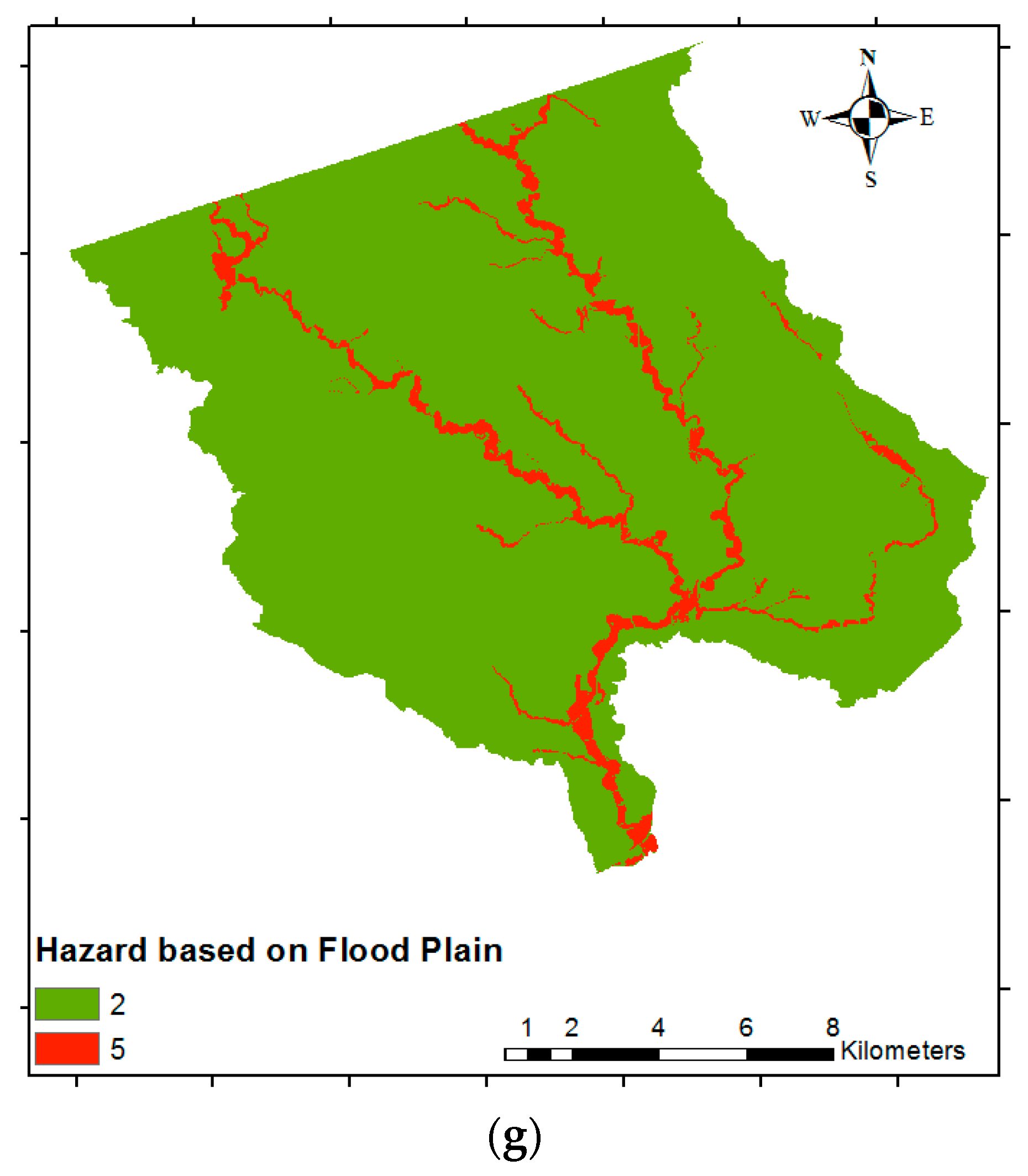
Only limited studies of flood risk assessment (which include hazard, social, and economic vulnerability) in the GTA have been developed. A previous study [18] (which serves as the basis of the present research) generated flood risk index maps using GIS through the spatial combination of the flood hazard, social, and economic vulnerability layers. The criteria used to generate the flood hazard map were slope, land depression, the floodplain map (provided by the Toronto and Region Conservation Authority, TRCA), and land cover. For the economic vulnerability, a spatial layer that identified large buildings was used. Finally, the social vulnerability was determined by identifying the vulnerable groups from the 2006 census data from Statistics Canada. The limitation of this study was the direct assignment of criteria weights, instead of using a weighting method in the context of MCDM. Assigning criteria weights in this way does not allow obtaining a suitable assessment, as there is no theoretical background that supports a consistent assessment. Another study by Abdalla [19] used a web-based three-dimensional (3D) GIS approach for flood risk assessment, in which the flood hazard was based on hydraulic models (using the software HEC-RAS) under hypothetical flow rates simulated using the Canadian Hydrographic Service. The footprint of buildings within the flood hazard area was used for analyzing the exposure. Although this approach provides a 3D view of the flood extent, it does not include the economic and social vulnerability. In this sense, this study is a flood hazard assessment instead of a flood risk assessment. Thus, there is a need to develop flood risk maps of the GTA to account for the social and economic vulnerability, with a consistent method to assign weights to the different criteria used.

1.3. Flood Risk Assessment Using GIS and MCDM

Flood risk assessment using the GIS-based multi-criteria methodology is a relatively new approach, and only a few studies have implemented it. A pilot study for the River Mulde in Saxony, Germany [8], was developed using the multi-attribute utility theory (MAUT) and a disjunctive approach was used to assign weights for four different criteria (economic risk, population, social hot spots, and environmental risk). The flood hazard was obtained through a quasi two-dimensional (2D) hydrodynamic model using HEC-RAS. For the economic risk, the land use and estimates of the value of assets were used along with depth–damage curves (using damage functions). The social risk was based on the population density map. Finally, the social hot spots used the surveyed locations of old people and children, schools, and hospitals [8]. Similar to AHP, MAUT is a very popular method in MCDM analysis. Nevertheless, MAUT is extremely data-intensive, as it requires a large amount of input data, and the weights are assumed by the decision maker instead of being calculated (as is the case in the proposed AHP process) [20].

A study from the Iskandar region in Malaysia [21] used a rating method for assessing criterion weights. The criteria selected for generating the flood susceptibility map included: distance from the main stream and river, elevation, slope, land use, cover type, distance to discharge channel, and population density. One of the limitations of this study is the use of the rating method, as it lacks the theoretical foundation, and thus is difficult to justify the meaning of the weights assigned to the criteria. A study for the Red River Delta, Vietnam [22] was more sophisticated in terms of the weighting method used and the criteria selected. Similar to in the present paper, the AHP was used as the weighting method. The criteria selected for evaluating the flood hazard, economic, social, and environmental vulnerability are more suitable than the previously listed studies; they are also more difficult to obtain. The flood hazard was based on flood depth, flood duration, and flood velocity. The economic vulnerability used the area of residential buildings, special-use buildings, public infrastructure, and agricultural area. As for the social vulnerability, the population density, risk perception, spiritual values, and income levels were selected. Lastly, the environmental vulnerability was based on pollution (from industries, waste matter, and stagnations of floodwaters), erosion, and open spaces. Hence, when assessing flood risk for large-scale areas or in regions that lack detailed information (as is often the case), these criteria are not possible to use or require more resources, which makes this methodology difficult to implement [22].

As mentioned above, some of the limitations of previous studies that use the GIS-based multi-criteria flood risk approach include criteria weighting methods that are not appropriate, or in some cases are not used at all. Moreover, the use of more complex criteria (which may be difficult to access or to generate), or conversely the use of very simple criteria can lead to unreliable flood risk maps. In addition, some studies do not consider the social component, which is very important for implementing mitigation measures that are aiming to reduce the number of people affected after a flood event.

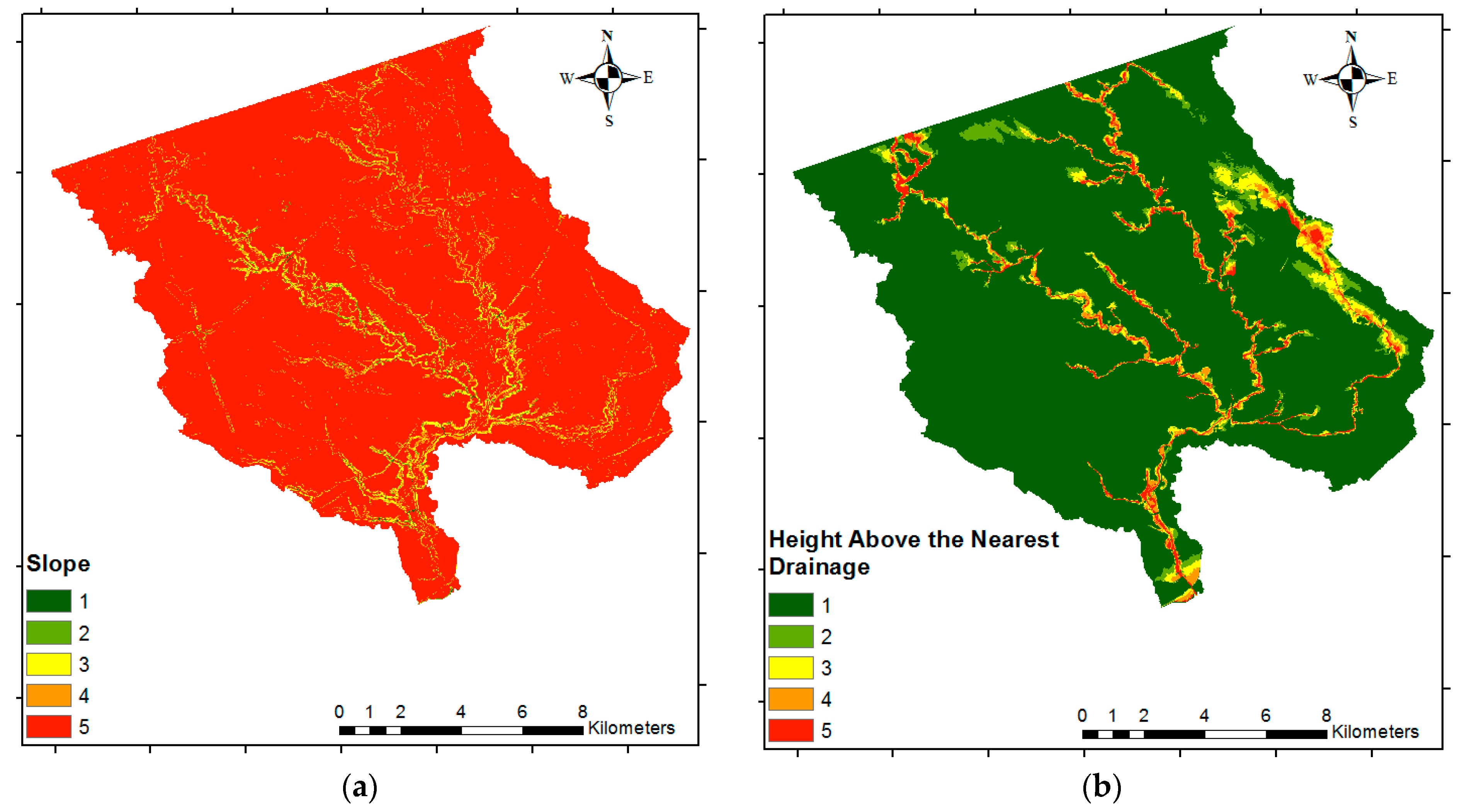
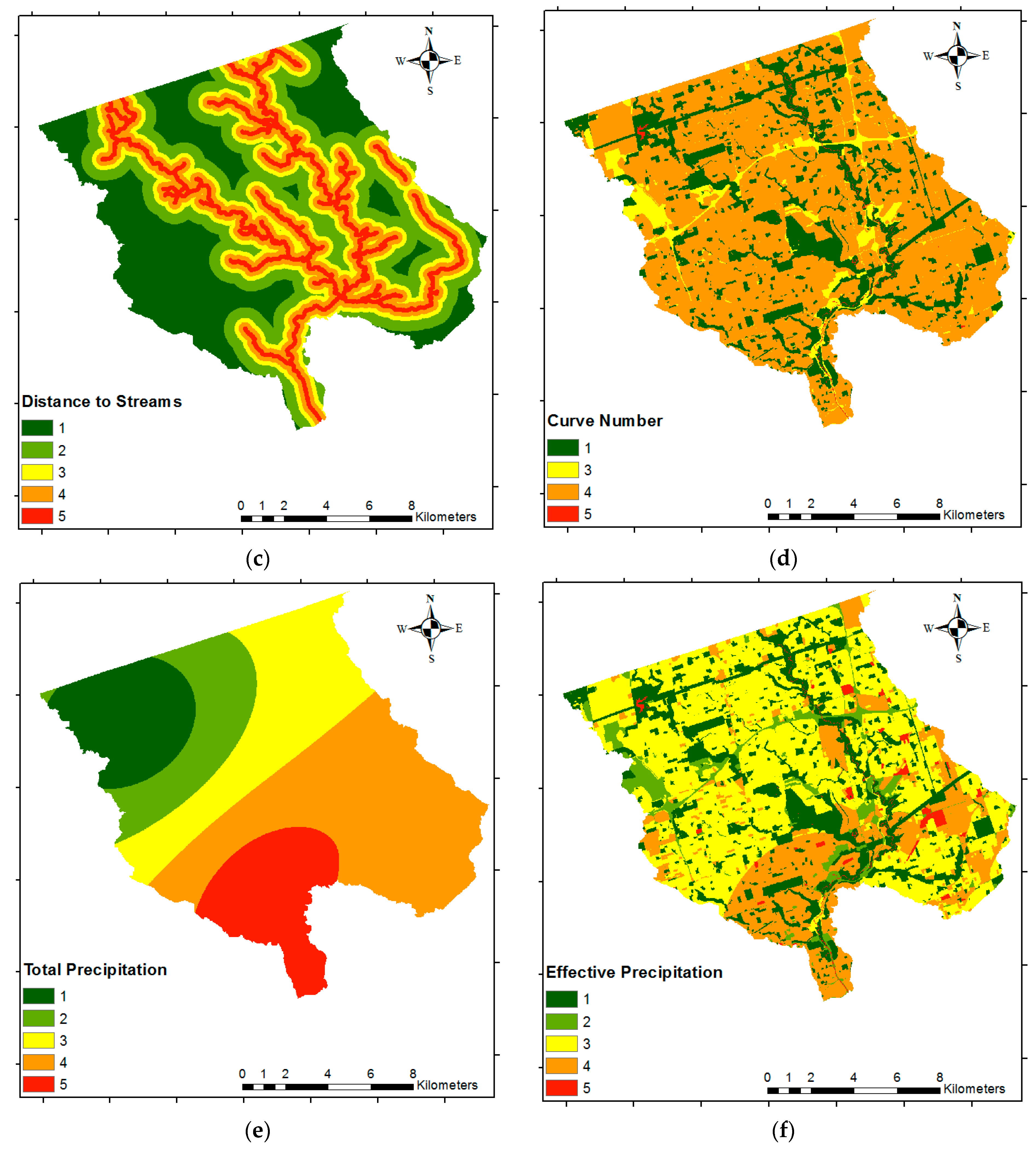
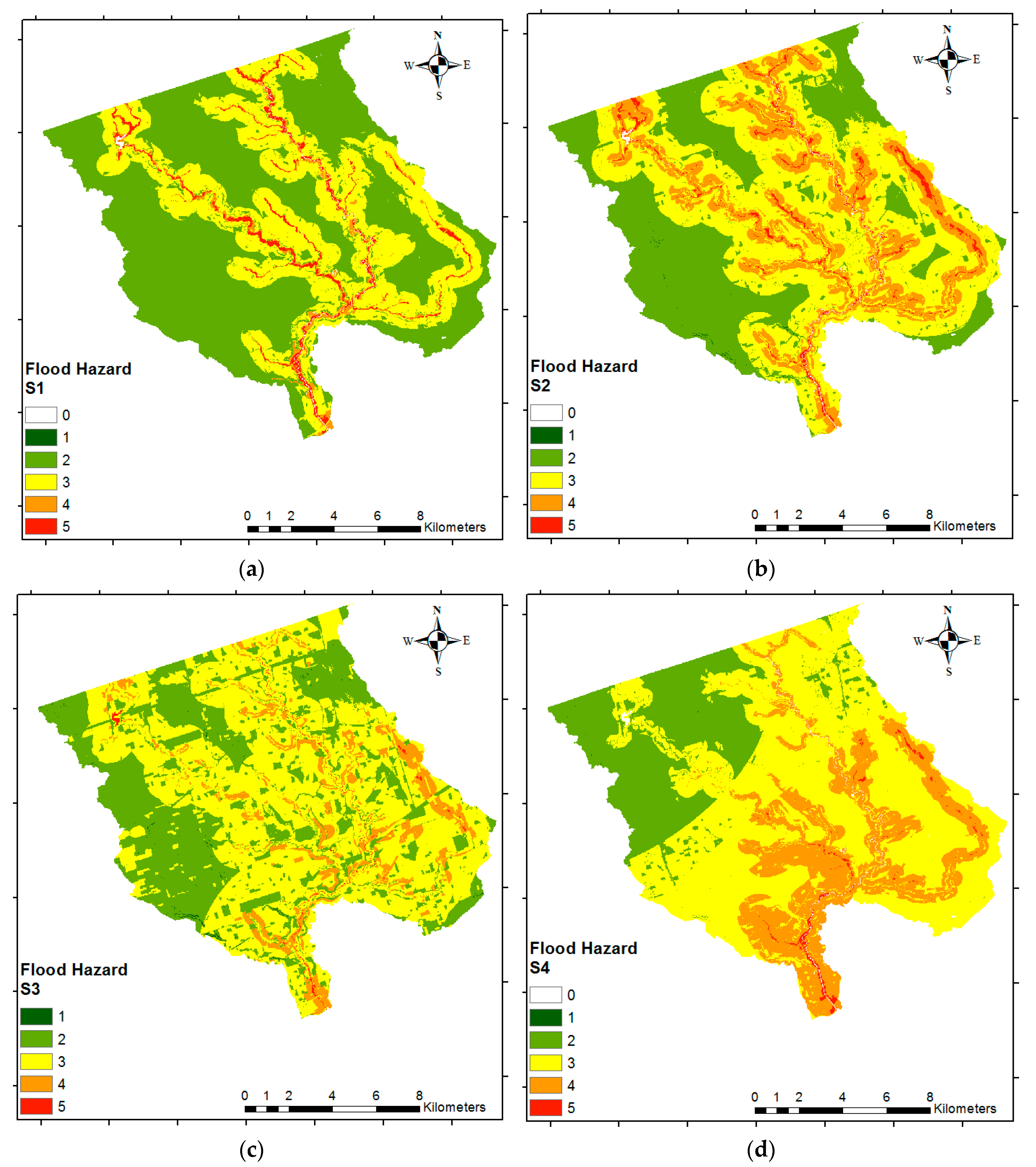
In the present paper, several improvements of the previous study for the GTA [18] are proposed. First, we implement MCDM as part of the methodology for determining the criteria weights. Second, we propose the use of more appropriate flood hazard parameters, including: distance to streams (DS), height above the nearest drainage (HAND), Curve Number (CN) (which is a widely used empirical parameter developed by the United States Department of Agriculture—Soil Conservation Service (SCS), and is commonly used in hydrology for predicting direct runoff [23]), total precipitation (TP), and effective precipitation (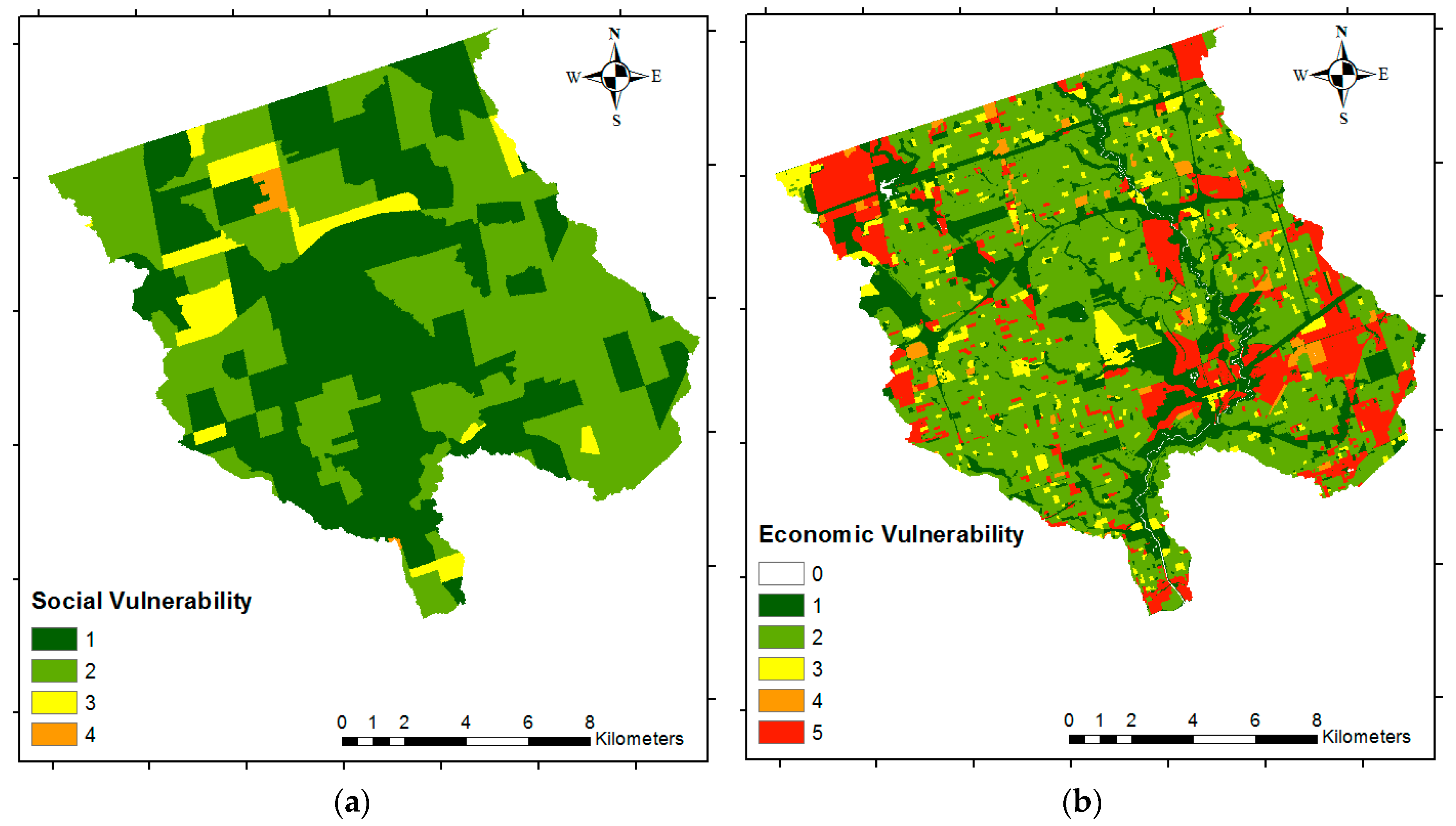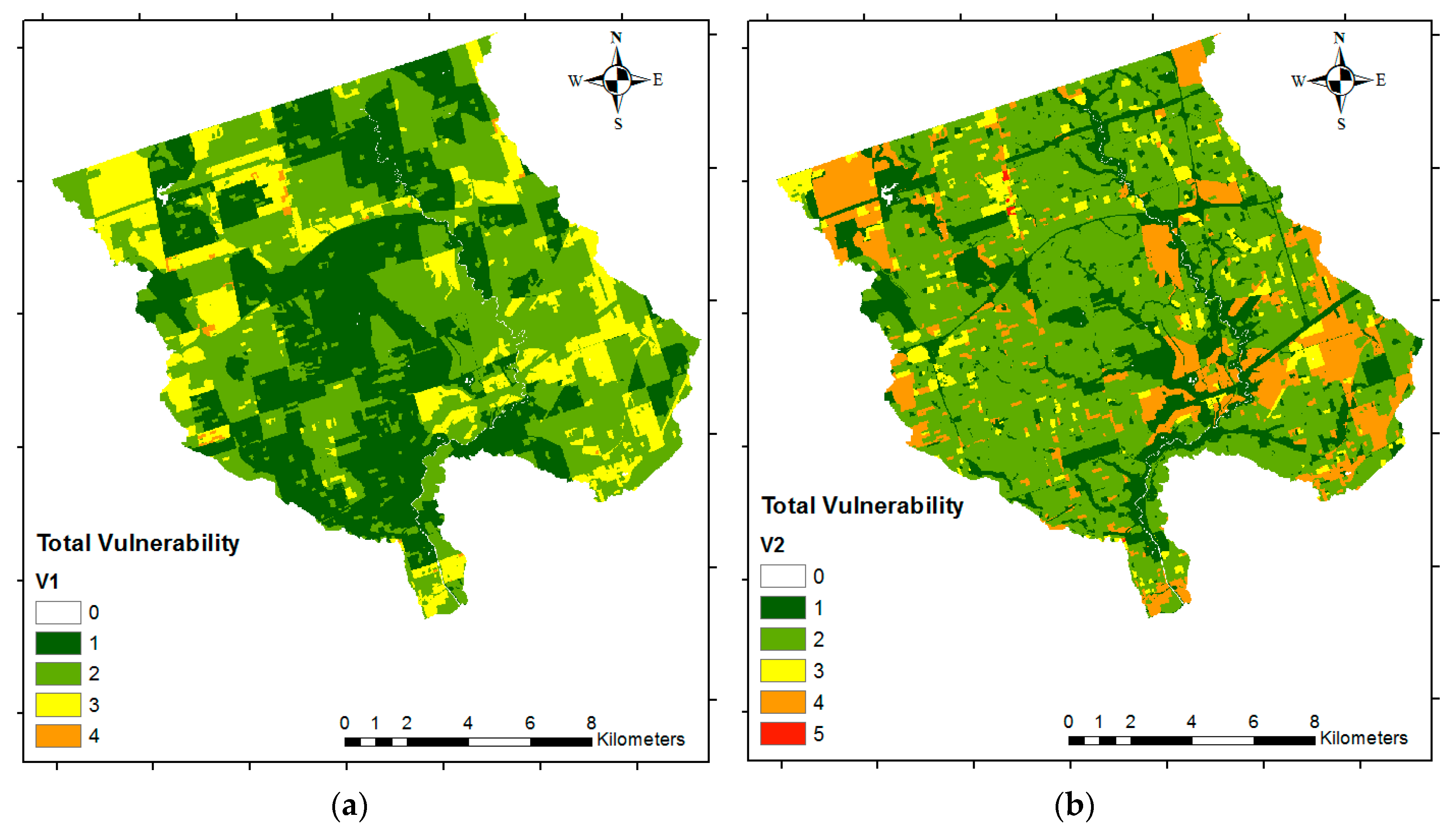EP). For economic vulnerability, we propose using land-use data instead of large buildings. Lastly, we use the most recent census data (2016) instead of using the previous census (2006) data for determining the social vulnerability. We then use the proposed methods to develop four different flood risk scenarios to demonstrate the utility of the proposed research.

Hence, the aim of the present study is to provide a reliable but simplified method for flood risk mapping based on GIS spatial analysis integrated with AHP, which assesses both the economic and social vulnerability. Furthermore, the current study aims to analyze the criteria that should be considered for each component (using pairwise comparison) in order to generate reliable flood risk maps using inputs that are just suitable and easy to access. The results of this research will provide enhanced flood risk maps for the GTA, compared with the previous studies, which do not include social or economic vulnerability, nor a methodology for calculating criteria weights. Additionally, this research introduces more suitable criteria for flood risk analysis. Note that while the method is demonstrated for a watershed in the GTA, the approach can be easily applied to other watersheds.

2. Materials and Methods

2.1. Study Area

The study area for this research was selected as the shared area between the GTA and the Don River watershed, which corresponds to an area of 202.6 km² (Figure 1). Precipitation data from four rain gauges (labeled HY008, HY016, HY021, and HY027) in Toronto were provided by the TRCA. The locations of the rain gauges are shown in Figure 1. The data showed that between 2009–2016, the months with the highest precipitation are typically from May to October, with an average rainfall of 82 mm/month, while the average rainfall from November to April is 29 mm/month (as illustrated in Figure 2). The Don River is one of the main watercourses that drains the GTA, running from Oak Ridges Moraine into Lake Ontario with a total length of about 100 km. It is composed of three main branches (East Don, West Don, and lower Don) and other two tributaries (Taylor/Massey Creek and German Mills Creek).

The GTA, with a population of about 6.4 million people in 2016, is the most densely populated metropolitan area in Canada. Furthermore, Toronto has experienced one of the fastest periods of growth in the last decades compared to other large and high-income metropolitan areas in the world. Since 1931, the population has increased 700% [24]. This rapid and sustained growth has made this region and watershed highly urbanized, with more than 75% of the area developed. Over the last 100 years, four significant flood events have occurred, and have significantly affected the area with fatalities, considerable economical losses, and infrastructural damage.

Table 1. A summary of the four major floods in Toronto.

Date	Intensity of Precipitation	Observations
15 October 1954 (Hurricane Hazel)	121 mm/12 h 210 mm/2 days	The most severe flooding in the Toronto area in 200 years. Great infrastructural damages 81 deaths, 7472 homeless 125.2 million dollars in damages
27 August 1976	75 mm/2 days	Destruction of 14 bridges 1.3 million dollars damages
19 August 2005	153 mm/3 h	100-year event 500 million dollars in damages The province’s most expensive natural disaster; the second costliest ever nationwide
8 July 2013	90 mm/2 h 126 mm/90 min	The power outages affected about 300,000 residents Transport disruptions 850 million dollars in damages.

summarizes some statistical information of these previous events, including the dates and intensity of the precipitation.

2.2. Overview of the Proposed Modeling Methodology

The applied methodology in this paper is a GIS-based multi-criteria approach for flood risk assessment based on the spatial intersection of three components: flood hazard, social vulnerability, and economic vulnerability. The AHP was selected as the criteria weighting method in the context of MCDM. The criteria used for determining the flood hazard are based on the parameters that most contribute to river floods (as identified in Section 1.3). The social vulnerability is based on the vulnerable groups from the 2016 Canadian census. Finally, the economic vulnerability is based on the land-use spatial layer.

The software used in this research is ArcMap (version 10.5.1, 2017), which is a popular GIS software that allows users to create, manipulate, and analyze geospatial data. The input data required for creating all of the maps were: the digital elevation model (DEM) map with a ground resolution of 5 m × 5 m (collected from [25]); soil type map [25]; the Don River watershed boundary map [26]; the GTA boundary map [27], land-use map [27], and streams map [27]; precipitation data from rainfall gauges provided by the TRCA; the floodplain map (provided by the TRCA); and the 2016 census data from Statistics Canada [28], along with the census tract boundaries.

Each of the criteria maps was transformed to the corresponding projected coordinate system (NAD_1983_UTM_Zone_17N) and converted to raster format. In addition, all of the maps were reclassified in a scale from 1 to 5, using the Reclassify Tool in ArcMap, where 1 refers to very low (e.g., low flood risk), and 5 is a very high level of flood risk. After reclassifying the maps, the Weighted Overlay Tool of ArcMap was used to carry out the spatial overlay of the maps. To illustrate how the Weighted Overlay Tool works, an example is shown in Figure 3 below.

After obtaining the weights, the cell of each input raster are multiplied by its corresponding weight, and then they are summed to obtain the output raster. For example, looking at the upper left cell, the input values are (i) (2 × 0.6) = 1.2 and (ii) (1 × 0.4) = 0.4. The output value then is 1.2 + 0.4 = 1.6. The final value is rounded to 2, since the weighted overlay output is an integer.

In order to analyze the influence of the criteria that contribute to flood susceptibility, four flood hazard scenarios were generated with different criteria (these scenarios are labelled S1, S2, S3, and S4, the details of which are provided below). Additionally, three total vulnerability scenarios were created that varied in the importance of its two components, the social and economic vulnerability (labelled V1, V2, and V3, and summarized below). The process of generating these hazard and vulnerability maps and final risk maps are detailed in the following sections.

2.3. Flood Hazard Spatial Layer

For developing the flood hazard layer, there is no consensus on the criteria that should be included [29]. Nevertheless, some of the criteria that contribute to flood susceptibility that are used in several studies [30] are: slope, distance from rivers, land use, and altitude. In the current research, slope and distance from rivers were included. However, land use was replaced by the USDA (United States Department of Agriculture) runoff Curve Number [23], while the altitude was replaced with the height above the nearest drainage point, as they have a higher influence in determining floods. Very few studies have included precipitation for mapping flood susceptibility under the GIS-based multi-criteria analysis [31,32]. Therefore, in this study, the total precipitation and effective precipitation (defined below) was also included in order to analyze the influence of these criteria. The floodplain map, provided by the TRCA, was also included in this research. This floodplain map was generated using extensive hydrologic and hydraulic models. The current study includes new criteria, and it also evaluates different flood scenarios by varying the criteria used to improve flood maps compared to previous studies, and the floodplain map generated by the TRCA. The criteria used are defined in detail below.

2.3.1. Slope (S)

The slope affects the velocity in which the water is conveyed through the drainage channel and the watershed. Additionally, the steeper the slopes, the higher the runoff will be, and consequently, higher peak discharges will be generated. The slope layer was derived from the DEM, with a resolution of 5 m × 5 m, using the Slope tool in ArcMap. It was reclassified in a scale from 1 to 5, where a value of 5 was given to lower slopes and 1 was given to higher values (details are shown in

Table 2. Classes of criteria that contribute to flood hazard. S: slope, HAND: height above nearest drainage, CN: Curve Number, TP: total precipitation, EP: effective precipitation, FP: floodplain.

Class	Level	Criteria for Flood Hazard
		S (Degree)	HAND (m)	DS (m)	CN	TP (mm)	EP (mm)	FP
5	Very high	≤10	≤2	≤100	94	>83.2	>65.1	In
4	High	10.1–20	2.1–4	101–300	90, 91	82.4–83.2	58.1–65.1	-
3	Medium	20.1–30	4.1–6	301–500	86	81.3–82.3	49.3–58.0	-
2	Low	30.1–50	6.1–8	501–1000	79	80–81.2	36.3–49.2	Out
1	Very low	>50	>8	>1000	74	≤79.9	≤36.2	-

).

2.3.2. Height Above Nearest Drainage (HAND)

The height above the nearest drainage has influence in flood susceptibility, since low-lying land adjacent to streams is more susceptible to be flooded than higher land. The map was generated with a previously developed tool by Dilts [33], which requires the DEM and the Streams layer as inputs. When reclassifying, lower values of HAND were assigned to a higher class, and higher values were assigned to a lower class, as shown in Table 2.

2.3.3. Distance to Streams (DS)

The measure of distance to streams plays an important role in defining areas susceptible to flooding. The zones closest to rivers are the most affected by floods. To obtain these distances, the Euclidean Distance tool was used in the Spatial Analyst Tools in ArcGIS. The reclassification was based on assigning a value of 5 to areas farthest from streams, and a value of 1 to areas near streams (as shown in Table 2).

2.3.4. Curve Number (CN)

The CN is an empirical parameter by the Soil Conservation Service (SCS) used in hydrology for predicting direct runoff or infiltration from rainfall excess. It considers the characteristics of land use and soil type. The values of CN ranged from 100 for impermeable surfaces to 30 for very permeable soils with low runoff potential. The CN map was obtained using both the land-use type data and the soil type. CN values are published by the SCS for different land uses and soil types [23]. As a high CN means high runoff and low infiltration and a low CN means low runoff and high infiltration, high values of CN where assigned to a scale of 5, and low values were assigned a CN value of 1 (details are provided in Table 2).

2.3.5. Total Precipitation (TP)

The precipitation is the major cause of river floods. Heavy rainfall can lead to flooding when the streams can no longer convey excess water. As runoff is related to the amount of precipitation, higher precipitations increases the amount of runoff. Therefore, higher precipitation leads to higher flood susceptibility. Daily precipitation data from four rain gauge stations in the Don River watershed, from 2009 to 2016, were used to create the precipitation-isohyet map generated by interpolating the monthly average precipitation data, for the wet season (May to October), using the inverse distance weighted (IDW) interpolation method. The TP map was reclassified on a scale from 1 (for low values of TP) to 5 (for high values of TP), as shown in Table 2.

2.3.6. Effective Precipitation (EP)

Effective precipitation represents the precipitation after losses (such as infiltration and evapotranspiration). It is calculated using the total precipitation and the CN at a given point using Equation (1) [34]:

$$EP=\frac{{\left[TP-\frac{5080}{CN}+50.8\right]}^2}{TP+\frac{\mathrm{20,320}}{CN}-203.2}$$

(1)

where $EP$ is the effective precipitation in mm, $TP$ is the precipitation of the storm in mm, and $CN$ is the Curve Number. Table 2 shows that high values of $EP$ were assigned to a scale of 5, and low values were assigned to a scale of 1.

2.3.7. Floodplain

The floodplain is the area adjacent to a stream that is prone to flooding during high discharge periods. This is the most important criteria for determining the flood hazard map. The floodplain for the Don River watershed was generated and provided by the TRCA using hydrological and hydraulic models. As this map only contains the area (boundary) of the floodplain, the reclassification consisted of assigning a value of 5 to all of the cells that are within the boundary, and a value of 2 (following the selection in [18]) to those that are outside the boundary.

2.3.8. Summary of the Flood Layer

In summary, the criteria taking into account for evaluating the flood hazard are: Slope (S), height above the nearest drainage (HAND), distance to streams (DS), Curve Number (CN), floodplain (FP), total precipitation (TP), and effective precipitation (EP). Table 2 presents the classes for each criteria, showing the ranges for each class. These classes were based on values from the literature (some examples are listed in Section 1.3) and professional expertise. These classes may be adjusted, as required, for different case studies or by decision makers. The values presented here are used to demonstrate the applicability of the proposed approach, but can be varied as required. Figure 4 presents the reclassified maps and highlights the levels from very low to very high for each criteria.

In order to determine which criteria are the most suitable, four scenarios were created with different combinations of the criteria (S1, S2, S3, and S4). Figure 5 shows the criteria selected for each scenario. S1 is selected as the base case, since it includes the base criteria (DS, HAND, S, CN) and the floodplain map, which is the most influential criteria in the flood hazard map, as it is based on hydrological and hydraulic models. S2 contains the same base criteria as S1, but not the floodplain map. S3 contains S, HAND, DS, and EP, but does not include the CN, as it is implicit in the calculation of effective precipitation. S4 contains the base criteria as well as TP. As mentioned above, these criteria are some of the most significant parameters to affect flood susceptibility. Additionally, TP and EP were included to determine whether or not the precipitation (which is the driver for flood hazard) is needed to generate food risk maps under the current methodology. The objective of developing scenarios S2, S3, and S4 is to determine if they can general flood risk maps that are comparable to the S1 map, since S1 used the detailed floodplain map from the TRCA. If these maps are indeed comparable, then it demonstrates that the proposed approach can create useful tools, with relatively low data requirements, as compared to S1.

2.4. Social Vulnerability Spatial Layer

The social exposure is based on the number of vulnerable groups in the area. The vulnerable groups were determined by age, family structure, language proficiency, income, education level, land tenure (i.e., renters), and population density (the corresponding indicators are listed in

Table 3. Criteria for social vulnerability.

Demographic Category	Indicators	Specific Indicators (Criteria)
Demographic characteristics	Age	People 75 years and older
		Children four years and younger
	Family structure	Lone parents
	Language proficiency	Non-English or French-speaking people
Socioeconomic status	Income	People with low income 1
	Education	High school education or less
Land tenure	Renters	Rented apartments
Neighborhood characteristics	Population density	Population density per km2

¹ Low income based on the Low-income measure, after tax (LIM-AT) provided by Census 2016.

). This information was obtained from the 2016 census tracts data [28]. These criteria for determining social vulnerability were selected based on a previous study [35], which reviewed 142 articles related to social vulnerability to flooding disasters. The study found that the category with the highest frequency of appearance was demographic characteristics (58%), followed by socioeconomic status (55%), health (45%), coping capacity (39%), risk perception (36%), neighborhood characteristics (30%), and land tenure (30%). Details of why the criteria were selected are described in the following sections.

2.4.1. Demographic Characteristics: Age, Family Structure, and Language Proficiency

Among all the demographic drivers of social vulnerability, age (very young and elderly people) has the highest number of citations within the literature review [35]. Their vulnerability is associated with their physical condition and dependency; therefore, their mobility is limited. The elderly are more affected due to their health condition, coping difficulties, and inability or reluctance to leave their place [36].

Family structure (such as lone parent families) is a useful measure of social vulnerability, since, e.g., families with lone parents have only one income, they have to deal with the financial costs by themselves. They also have to support their children, meet their basic needs, and deal with the stress without the support of a partner [37]. Lastly, language proficiency is a measure of social vulnerability that affects people in all the stages of the disaster, as they cannot be well-informed about the warnings, evacuations, and resources for recovery [36].

2.4.2. Socioeconomic Status: Income and Education

People with low income have less access to resources, suffer from more stress, and have less coping capacity [38]. They also suffer from more health impacts than people with higher incomes. Finding a temporary accommodation is more difficult and is often not possible [39]. Lower education is associated with poverty, unemployment, and overpopulation [35]. Therefore, this group is vulnerable to flooding due to their low coping capacity after a flood event.

2.4.3. Land Tenure and Neighborhood Characteristics

Renters (a type of land tenure) often suffer from more stress and health problems than homeowners [40]. Additionally, compared to owners, renters are less aware of flood risks, have a lower understanding of warnings, take less action to reduce damage, have less control over protective measures and repairs, and have higher inundation levels [41]. The population density of a neighborhood is often linked with lower income housing placed in floodplain areas [42]. Furthermore, overcrowded neighborhoods are more likely to have poor drainage systems and infrastructure [43]. People from neighborhoods with these characteristics face difficulties in evacuating quickly and have a higher risk of disease transmission [44].

2.4.4. Summary of Social Vulnerability

To sum up, the social vulnerability included was based on eight criteria identified in Table 3. The data obtained by Statistics Canada was the boundary of the census tract, in a shapefile format (polygons), and the census data was a dBase (dBF) file. After joining the shapefile with the dBase file, the resulting map was transformed into a raster file, which then was divided into individual rasters for each criterion (thus, eight rasters in total). Each raster was then reclassified on a scale from 1 to 5, assigning higher levels of vulnerability to a higher percentage of the population belonging to each criterion. The levels used for all of the social vulnerability criteria are shown in

Table 4. Classes of criteria that contribute to social vulnerability.

Class	Level	Population for Each Criterion %
5	Very high	>80
4	High	61–80
3	Medium	41–60
2	Low	21–40
1	Very low	≤20

.

2.5. Economic Vulnerability Spatial Layer

The physical exposure refers to man-made infrastructure elements that are exposed to damages due to flooding [18]. Generally, these physical damages are measured in terms of economic losses. For this, the required information includes: property value, structural type, and height of the buildings. As an approach to estimate the vulnerability of properties in terms of economic losses, the land-use layer was used. A previous study [45] developed for flood risk assessment in Canada, at a national scale, also used land use as an indicator of property value.

The land-use map was reclassified into a scale from 1 to 5 according to their economic value. In this study, the Resource and Industrial land-use type was established as the one with the highest economic value, while parks, recreational, and open areas were assigned the lowest. The classification system used for economic vulnerability is shown in

Table 5. Classes for economic vulnerability.

Class	Level	Land Use
5	Very high	Resource and industrial
4	High	Commercial
3	Medium	Government and institutional
2	Low	Residential
1	Very low	Parks and recreational, open area

.

The total vulnerability was generated for three scenarios: V1 where the social vulnerability was given a higher importance than economic vulnerability (67% versus 33%), V2, which represented the opposite case (33% versus 67%), and V3, in which both were equally important (50% for both of them).

2.6. Determining Criteria Weights

AHP, developed by Saaty in 1990 [10], is one of the several criteria weighting methods of MCDM. This method allows comparing two criteria at a time through a pairwise comparison matrix in which the values of relative importance from one criterion over another criterion are assigned. It provides a measure of a level of consistent judgment supported by a theoretical background. The standardized scale of relative importance ranges between 1 and 9, where 1 is equal importance, and 9 is extreme importance (the details are provided in

Table 6. Saaty’s scale for weight assignment [10].

Intensity of Importance	Definition
1	Equal importance
2	Equal to moderate importance
3	Moderate importance
4	Moderate to strong importance
5	strong importance
6	Strong to very strong importance
7	very strong importance
8	Very to extremely strong importance
9	Extreme importance

). AHP has been used worldwide in a wide range of fields such as industry, education, transportation, and healthcare, among others, especially due to its application in group decision making [11].

This method has been increasingly applied in flood management. In a case study in Eldoret Municipality (Kenya), AHP was used to determine the flood vulnerable areas, in which through a validation process, it was found that the AHP-GIS-based results were reliable with a 92% of accuracy when compared with the simulated results (HEC-RAS simulation) [46]. Similarly, in a case study in the Yasooj River (Iran) [23], the authors used AHP to identify the potential flood hazard zones; the method was validated against an inundation simulation (conducted using HEC-RAS), and it showed the reliability of the flood hazard map. A study conducted in Terengganu (Malaysia) used AHP to generate a map of flood susceptibility areas, and found a significant similarity when compared with an original flood map obtained from the Department of Irrigation and Drainage [47].

Besides the AHP, there are other methods for determining criteria weights such as the Fuzzy Multi-Criteria Decision Making Process (FDM), multi-attribute utility theory (MAUT), SMARTER, rank order, weighted summation, Electré, Regime, and Evamix, amongst others [48]. The random forest, which is an ensemble learning method of n tree-based classifiers, is an alternative method that was used in a study case in Germany to identify variables that influence damages and model flood damages [49]. The AHP method presents many advantages: it is appropriate for group decision making; it works with both quantitative and qualitative input data; the stakeholders can answer the pairwise question easily; it allows a hierarchical configuration of the criteria; it enables evaluating the consistency of preference; and it provides a measure of a level of consistent judgment supported by a theoretical background.

The first step for determining the criteria weights under the AHP method is to create a pairwise comparison matrix for the criteria selected, in which the values of relative importance from one criterion over another criterion are assigned on a scale from 1 to 9. The pairwise comparison matrix for flood hazard, social and economic vulnerability was based on the literature review and self-criteria from professional experience. The complete detailed pairwise matrices are included in Appendix A for reference.

In order to provide a better understanding of the methodology, the calculation procedure of criteria weights for scenario S2 is presented here as an example. The first step in calculating the criteria weights is to establish the order preference and assign the intensity of importance for the selected pair of criteria based on the scale presented in Table 6.

Table 7. Assigning the importance score. S: slope.

Pair of Criteria	Importance Score
DS > HAND	2
DS > S	2
DS > CN	3
HAND > S	1
HAND > CN	2
S > CN	2

summarizes this for scenario S2; here, DS and HAND are given an important score of 2, which translates to equal to moderate importance using the scale in Table 6. The next step is to build the pairwise comparison matrix where in each cell, every criterion is assigned an intensity of importance over another. Each criterion are compared with the other criteria (see

Table 8. Procedure for weights calculation for a sample case.

Criterion	Comparison Matrix				Normalization				Weights
	DS	HAND	S	CN	DS	HAND	S	CN
DS	1	2	2	3	1/2.33 = 0.43	0.44	0.44	0.38	(0.43 + 0.44 + 0.44 + 0.38)/4 = 0.42
HAND	1/2	1	1	2	0.21	0.22	0.22	0.25	0.23
S	1/2	1	1	2	0.21	0.22	0.22	0.25	0.23
CN	1/3	1/2	1/2	1	0.14	0.11	0.11	0.13	0.12
∑	2.33	4.50	4.50	8.00	1.00	1.00	1.00	1.00	1.00

). The next step consists of a linear normalization of the pairwise comparison matrix: all of the values from each column are summed, and then each element of the matrix is divided by its total. Finally, the weights are obtained by computing the average of each row of the normalized values of the matrix (Table 8).

Since the AHP may have inconsistencies in establishing the values for the pairwise comparison matrix, it is important to calculate this level of inconsistency using the consistency index (CI), which should be less than 0.1. To calculate the $CI$, the first step is to calculate the weighted sum vector by multiplying the weight of the criteria with the pairwise comparison values (shown in Appendix A for all four scenarios). Then, the consistency vector is calculated as the ratio between the weighted sum vector and the weights and finally lambda ($\lambda$), which is the average of the consistency vector, is also calculated.

Table 9. Weighted sum vector and consistency vector.

Criterion	Weighted Sum Vector	Consistency Vector
DS	(0.42) × (1) + (0.23) × (2) + (0.23) × (2) + (0.12) × (3) = 1.69	1.69/0.42 = 4.016
HAND	0.911	4.010
S	0.911	4.010
CN	0.491	4.005

shows a sample calculation for the values. The value of $\lambda$ and the number of criteria ($n$) are used in Equation (2) to calculate the $CI$ [10]:

$$CI=\frac{\lambda -n}{n-1}$$

(2)

The average of the consistency vector ($\lambda$) is simply the arithmetic mean of the consistency vector from Table 9, and a sample calculation is included below. Then, Equation (2) is used where $n$ = 4 (since there are four criteria) to determine $CI$, which in this example indicates a high level of consistency, since it is less than 0.1.

$$\lambda =\frac{4.016+4.010+4.010+4.005}{4}=4.010$$

$$CI=\frac{\lambda -n}{n-1}=\frac{4.010-4}{4-1}=0.00345$$

2.7. Flood Risk Spatial Layer

The flood risk map is generated by a spatial layer overlay operation between the flood hazard map and the total vulnerability (social vulnerability and economic vulnerability), i.e., the consequences. The flood risk map ($R_{FSV}$) based on flood hazard ($H_F$) and social vulnerability $\left(V_S\right)$ is derived from Equation (3):

$$R_{FSV}=H_F\cap V_S$$

(3)

The flood risk map $(R_{FEV})$ based on flood hazard ($H_F$) and economic vulnerability $\left(V_E\right)$ is derived from Equation (4):

$$R_{FEV}=H_F\cap V_E$$

(4)

The total vulnerability map $\left(V_T\right)$ is derived from Equation (5):

$$V_T=W_S{V}_S\cap W_E{V}_E$$

(5)

where $W_S$ is the weight of the social vulnerability, and $W_E$ is the weight of the economic vulnerability. Similarly, the flood risk map $(R_{FTV})$ based on flood hazard and total vulnerability is derived from Equation (6).

$$R_{FTV}=H_F\cap V_T$$

(6)

2.8. Comparison of Scenarios

In order to determine the scenario that best suits the base case, a comparison was made between each scenario and the base case using Equation (7).

$$RC=R{S}_1-R{S}_n$$

(7)

where $R{S}_1$ is the risk map under the scenario S1, and $R{S}_n$ is the risk map for each scenario (being $n$ = 2, 3, and 4), and $RC$ is the risk change between S1 and the other scenarios. The results from Equation (7) can take values from −4 to +4, where negative values indicate a higher scale of $R{S}_n$, meaning an overestimation of the risk compared to the base case (S1), and positive values indicate a higher scale of $R{S}_1$, and thus an underestimation of the risk. Hence, values of $RC$ that are equal or close to zero indicate a best approximation to the base case. The risk change maps were generated for each vulnerability scenario (V1, V2, and V3). Additionally, from the risk change maps, the percentage area of each RC value were obtained.

3. Results and Discussion

3.1. Generation of Flood Hazard Maps

Table 10. Weights of flood hazard criteria for each scenario.

S1		S2		S3		S4
Criteria	Weight (%)	Criteria	Weight (%)	Criteria	Weight (%)	Criteria	Weight (%)
Floodplain	45	DS	42	EP	42	TP	36
DS.	22	HAND	23	DS	27	DS	25
HAND	13	S	23	HAND	16	HAND	16
S	12	CN	12	S	15	S	14
CN	8	-	-	-	-	CN	9
CI	0.022	CI	0.003	CI	0.015	CI	0.019

shows the weights of the criteria selected for each flood hazard scenario and their corresponding value of $CI$. These weights were used to generate the flood hazard maps for each scenario (Figure 6). The flood hazard for S1 (the base case) shows a higher susceptibility to floods in the surroundings of the streams (the closer to the stream, the higher the susceptibility). The flood hazard for S2 also presents areas of high susceptibility in the surroundings of the streams, but with a higher buffer distance from the streams, i.e., a larger area in yellow surrounding the streams. S3 is dominated with areas of medium susceptibility (yellow), some areas close to the river with high susceptibility, and just a few regions with very high susceptibility (red). Zones of higher effective precipitation are reflected in areas with higher susceptibility. S4 shows high and very high susceptibility in a much wider buffer distance from streams, compared to the other scenarios, and medium and low susceptibility are clearly marked by the level of precipitation. Generally speaking, these maps show that the map generated in S2 is closest to S1 (the base case map that uses detailed hydrologic and hydraulic models). This means that the simple criteria used for S2 (DS, HAND, S, and CN) can adequately reproduce the flood hazard maps generated in S1.

3.2. Generation of Vulnerability Maps

The weights of social vulnerability (shown in

Table 11. Weights of social vulnerability criteria.

Number	Criteria	Weight (%)
1	People 75 years and older	18
2	Children four years and younger	17
3	Lone parents	16
4	Non-English or French-speaking people	15
5	People with low income	11
6	High school education or less	9
7	Population density per km2	8
8	Rented apartments	6
CI		0.046

) were assigned to the corresponding criterion to generate the social vulnerability map (Figure 7a). As the economic vulnerability is based on only one criterion (land use), no pairwise comparison was needed to calculate the weights. Instead, the classes established in Table 5 were used directly (with the results presented in Figure 7b). The weights of total vulnerability for each scenario are shown in

Table 12. Weights of total vulnerability criteria for each scenario.

V1		V2		V3
Criteria	Weight (%)	Criteria	Weight (%)	Criteria	Weight (%)
Social	67	Social	33	Social	50
Economic	33	Economic	67	Economic	50
CI	0	CI	0	CI	0

. Finally, the total vulnerability maps (shown in Figure 8) for each scenario, V1, V2, and V3, were derived from the combination of social vulnerability and economic vulnerability, by applying the weights determined for each scenario (Equation (5)). These figures show that the economic vulnerability has a higher impact on the total vulnerability: there are relatively more high total vulnerability zones when the economic vulnerability is given higher priority as compared to when social vulnerability is given higher priority.

3.3. Generation of Flood Risk Maps

Flood risk maps were generated as a spatial overlay (equal weights) between the total vulnerability maps (either V1, V2, or V3) and the flood hazard maps (S1, S2, S3, and S4), and these maps are shown in Figure 9. These maps were generated by combining the flood hazard maps with the total vulnerability. Generally speaking, scenario S2 was the most similar to the base case scenario S1 (due to the similarity between the flood hazard maps). For each hazard scenario, a higher risk is seen when economic vulnerability is given higher priority (V2) than the other two cases: there are more regions with medium (yellow) or higher risks (orange and red) than the cases where social vulnerability is given priority (V1) or has equal priority (V3). This is expected, since there are more economically vulnerable regions in the study area (based on Figure 7b) than social vulnerable regions (Figure 7a); in fact, there are no socially vulnerable areas with a very high (red) risk—a consequence of the selected criteria, pairwise comparison, and available data.

Comparison Flood Risk Maps

A process of validation is essential when modeling, as it confirms if the model is representing the reality or observations sufficiently. Since there are no previous flood risk maps in the study area to directly validate the flood risk maps generated in this research, the flood risk maps for scenarios S2, S3, and S4 were compared to the base case (S1). Scenario S1 is considered the most reliable scenario, since it includes the floodplain map (generated and provided by the TRCA as a criterion). This validation approach was made between the different flood scenarios and the different social vulnerability scenarios (V1, V2, and V3).

Figure 10 shows the percentage of the total area that corresponds to each RC value, as obtained from Equation (7), for each flood and vulnerability scenario. An analysis of this figure indicates that overall, S2 is the most similar scenario to the base case (S1), followed by S3 and S4. The scenario S2 is where there is a minimum difference from S1. For the scenarios where more importance is given to the social vulnerability (scenario V1), S2 and S3 present similar results in terms of likeness to the base case, as the percentage of the areas with the same risk scale as the base case were around 80% for both scenarios. The difference between S2 and S3 relies on that the former tends to overestimate the risk scale, and the latter tends to underestimate it. In contrast, S4 presents 70% in the areas with the same risk scale as the base case, and overestimates much more of the risk scale in comparison with the other scenarios.

When giving more importance to the economic vulnerability (scenario V2), S2 is by far the best scenario, as it has the highest percentage of area with same risk scale as the base case, followed by S2 and S3 (around 98%, 70%, and 62%, respectively). When giving equal importance to the social and economic vulnerability (scenario V3), S2 also has the highest percentage of area with the same risk scale as the base case, followed by S3 and S4 (around 75%, 70%, and 61%, respectively). S3 and S4 underestimate almost the same percentage area (around 24% for both), and overestimate a minimum.

Figure A1 (Appendix B) shows the flood risk change maps for the vulnerability scenarios V1, V2, and V3, respectively, where the grey colored regions represents equal values of risk between the base case and each flood scenario, blue represents an underestimation, and red represents an overestimation of the risk scale. From Figure A1, it is clear that S4 is the least similar scenario compared to the base case scenario, presenting larger areas of higher risk than the base case. Most of the areas where the risk is overestimated correspond to the areas of higher precipitation.

4. Conclusions

The flood risk mapping based on GIS and multi-criteria analysis is a valuable tool for estimating areas prone to flood risk, and help water resources planners and decision makers to focus on specific areas in order to perform a further detailed assessment of flood risk (e.g., through the use of hydrological and hydraulic models). Consequently, this simplified but reliable methodology can help the reduce resource requirements for fairly accurate flood risk assessments.

Some of the advantages of this approach are its flexibility, ease of handling, and low cost, making it possible to apply it to areas where there is a lack of detailed information, when the aim is to obtain large-scale flood risk maps, or when the policy makers require a rapid flood risk assessment. The use of AHP as the weighting criterion method presents several advantages as well, such as emphasizing the structure of the preferences of the decision makers among a number of criteria. Thus, instead of selecting the “best” alternative, this method provides the basis and tools for intelligent decision-making, allowing decision makers to obtain the alternative that best suits their needs. It is also important to note that S2 is very similar to S1 (based on the comparisons presented above), but was generated with much less data (i.e., did not require the intensive hydrological and hydraulic models used to generate the floodplain map used in S1).

In addition, by changing the weights of vulnerability (both social and economic), it is possible to obtain different risk maps based on a higher, lesser, or equal importance of one vulnerability over another. This allows managers to take action on the main objective as they have deemed best, e.g., focus on either reducing the number of people affected (i.e., social vulnerability) or the economic losses.

The results of the study show that for flood hazard mapping, only the criteria of distance to streams, slope, height above the nearest drainage, and CN are enough to obtain reliable maps. However, if the precipitation data is included, it is better to use the effective precipitation rather than using the total precipitation. In this sense, the inputs required are the DEM, soil type, and the streams layer. The flood risk maps generated in this study can be very helpful for the City of Toronto or the TRCA to implement required mitigation measures for insurance purposes, disaster response, and land management. The proposed approach is easily extended to other jurisdictions to determine flood risk maps using indicators or criteria that are available. An improvement on the current methodology would be to use the fuzzy majority approach proposed by [50] for GIS-based multi-criteria analysis.

References

1. Zwenzner, H.; Voigt, S. Improved estimation of flood parameters by combining space based SAR data with very high resolution digital elevation data. Hydrol. Earth Syst. Sci. Discuss. 2008, 5, 2951–2973. [Google Scholar] [CrossRef]
2. National Geographic. Floods. Available online: https://www.nationalgeographic.com/environment/natural-disasters/floods/ (accessed on 15 April 2018).
3. Nelson, S.A. Flooding Hazards, Prediction & Human Intervention; Tulane University: New Orleans, LA, USA, 2015. [Google Scholar]
4. Sole, A.; Giosa, L.; Albano, R.; Cantisani, A. The laser scan data as a key element in the hydraulic flood modelling in urban areas. Int. Arch. Photogramm. Remote Sens. Spat. Inf. Sci. 2013, 42, 65–70. [Google Scholar] [CrossRef]
5. Samela, C.; Albano, R.; Sole, A.; Manfreda, S. An open source GIS software tool for cost effective delineation of flood prone areas. Comput. Environ. Urban Syst. 2018, 70, 43–52. [Google Scholar] [CrossRef]
6. Peduzzi, P.; Dao, H.; Herold, C.; Mouton, F. Assessing global exposure and vulnerability towards natural hazards: The Disaster Risk Index. Nat. Hazards Earth Syst. Sci. 2009, 9, 1149–1159. [Google Scholar] [CrossRef]
7. Albano, R.; Mancusi, L.; Abbate, A. Improving Flood Risk Analysis for effectively supporting the implementation of flood risk management plans: The case study of “Serio” Valley. Environ. Sci. Policy 2017, 75, 158–172. [Google Scholar] [CrossRef]
8. Meyer, V.; Haase, D.; Scheuer, S. Flood risk assessment in European river basins-concept, methods, and challenges exemplified at the Mulde River. Integr. Environ. Assess. Manag. 2009, 5, 17–26. [Google Scholar] [CrossRef] [PubMed]
9. Malczewski, J.; Rinner, C. Introduction to GIS-MCDA. In Multicriteria Decision Analysis in Geographic Information Science; Springer Science + Business Media: New York, NY, USA, 2015; pp. 23–55. ISBN 978-3-540-74757-4. [Google Scholar]
10. Saaty, T.L. How to Make a Decision: The Analytic Hierarchy Process. Eur. J. Oper. Res. 1990, 48, 9–26. [Google Scholar] [CrossRef]
11. Majumer, M. Multi Criteria Decision Making. In Impact of Urbanization on Water Shortage in Face of Climatic Aberrations; Springer: New York, NY, USA, 2015; pp. 35–48. ISSN 2194-7244. [Google Scholar]
12. Chan, W.; Armenakis, C. 3D Building Evacuation Route Modelling and Visualization. Int. Arch. Photogramm. Remote Sens. Spat. Inf. Sci. 2014, 40, 221–226. [Google Scholar] [CrossRef]
13. Albano, R.; Mancusi, L.; Sole, A.; Adamowski, J. FloodRisk: A collaborative free and open-source software for flood risk analysis. Geomat. Nat. Hazards Risk 2017, 8, 1812–1832. [Google Scholar] [CrossRef]
14. Toronto Star. Hurricane Hazel Was Toronto’s Perfect Storm, by Vjosa Isai. 15 October 2016. Available online: https://www.thestar.com/news/gta/2016/10/15/hurricane-hazel-was-torontos-perfect-storm.html (accessed on 10 March 2018).
15. Toronto Star. Toronto’s July Flood Listed as Ontario’s Most Costly Natural Disaster, by Carys Mills. 14 August 2013. Available online: http://www.thestar.com/business/2013/08/14/july_flood_ontarios_most_costly_natural_disaster.html (accessed on 10 March 2018).
16. Bonell, J.L. Remembering the Don. In Reclaiming the Don: An Environmental History of Toronto’s Don River Valle; University of Toronto Press: Toronto, ON, Canada, 2014; pp. 173–188. [Google Scholar]
17. Armenakis, C.; Nipurama, N.; Montpetit, M. Is flooding in Toronto a concern? Nat. Hazards 2014, 72, 1259–1264. [Google Scholar]
18. Armenakis, C.; Du, E.X.; Natesan, S.; Persad, R.A.; Zhang, Y. Flood risk assessment in urban areas based on spatial analytics and social factors. Geosciences 2017, 7, 123. [Google Scholar] [CrossRef]
19. Abdalla, R. Distributed GIS Approach for Flood Risk Assessment. Int. J. Adv. Secur. 2009, 2, 182–189. [Google Scholar]
20. Velasquez, M.; Hester, P.T. An Analysis of Multi-Criteria Decision Making Methods. Int. J. Oper. Res. 2013, 10, 55–66. [Google Scholar]
21. Yeganeh, N.; Sabri, S. Flood Vulnerability Assessment in Iskandar Malaysia Using Multi-criteria Evaluation and Fuzzy Logic. Res. J. Appl. Sci. Eng. Technol. 2014, 8, 1794–1806. [Google Scholar] [CrossRef]
22. Dang, N.M.; Babel, M.S.; Luong, H.T. Evaluation of food risk parameters in the Day River Flood Diversion Area, Red River Delta, Vietnam. Nat. Hazards 2010, 56, 169–194. [Google Scholar] [CrossRef]
23. United States Department of Agriculture. Urban Hydrology for Small Watersheds Technical Release 55. Natural Resources Conservation Services. Conservation Engineering Division; 1986. Available online: https://www.nrcs.usda.gov/Internet/FSE_DOCUMENTS/stelprdb1044171.pdf (accessed on 26 July 2018).
24. Newgeography. The Evolving Urban form: Toronto. Available online: http://www.newgeography.com/content/003715-the-evolving-urban-form-toronto (accessed on 6 May 2018).
25. Giscoedata. Available online: http://www.giscoedata.lrc.gov.on.ca (accessed on 6 February 2018).
26. Ontario Ministry of Natural Reosurces. Available online: http://geo1.scholarsportal.info/#r/details/_uri@=834889117 (accessed on 6 May 2018).
27. DMTI Spatial Inc. Available online: http://geo.scholarsportal.info/#r/details/_uri@=41643035 (accessed on 6 February 2018).
28. Statistics Canada. Census Tracts. 2016. Available online: http://www12.statcan.gc.ca/census-recensement/2011/geo/bound-limit/bound-limit-2016-eng.cfm (accessed on 5 February 2018).
29. Tehrany, M.S.; Lee, M.; Pradhan, B.; Jebur, M.N.; Lee, S. Flood susceptibility mapping using integrated bivariate and multivariate statistical models. Environ. Earth Sci. 2014, 72, 4001–4015. [Google Scholar] [CrossRef]
30. Rahmati, O.; Zeinivand, H.; Besharat, M. Flood hazard zoning in Yasooj region, Iran, using GIS and multi-criteria decision analysis. Geomat. Nat. Hazards Risk 2016, 7, 1000–1017. [Google Scholar] [CrossRef]
31. Gaňová, L.; Zeleňáková, M.; Purcz, P.; Kuzevičová, Ž.; Hlavatá, H. A rainfall distribution and their influence on flood generation in the eastern Slovakia. Acta Univ. Agric. Silvicult. Mendel. Brun. 2013, 61, 1645–1652. [Google Scholar] [CrossRef]
32. Yahaya, S.; Ahmad, N.; Abdalla, R.F. Multicriteria Analysis for Flood Vulnerable Areas in Hadejia-Jama’are River Basin, Nigeria. Eur. J. Sci. Res. 2010, 45, 71–83. [Google Scholar]
33. Dilts, T. University of Nevada Reno. Available online: http://www.arcgis.com/home/item.html?id=b13b3b40fa3c43d4a23a1a09c5fe96b9 (accessed on 8 February 2018).
34. Chow, V.T.; Maidment, D.R.; Mays, L.W. Surface Water. In Applied Hydrology, 1st ed.; McGraw-Hill Science: Columbus, OH, USA, 1988; pp. 127–166. [Google Scholar]
35. Rufat, S.; Tate, E.; Burton, C.G.; Maroof, A.S. Social vulnerability to floods: Review of case studies and implications for measurement. Int. J. Disaster Risk Reduct. 2015, 14, 470–486. [Google Scholar] [CrossRef]
36. Coninx, I.; Bachus, K. Integrating Social Vulnerability to Floods in a Climate Change Context; Higher Institute for Labour Studies, Catholic University of Leuven: Leuven, Belgium, 2007. [Google Scholar]
37. Tapsell, S.M.; Penning-Rowsell, E.C.; Tunstall, S.M.; Wilson, T.L. Vulnerability to flooding: Health and social dimensions. Philos. Trans. R. Soc. 2002, 360, 1511–1525. [Google Scholar] [CrossRef] [PubMed]
38. Adger, W.N.; Kelly, P.M. Social vulnerability to climate change and the architecture of entitlements. Mitig. Adapt. Strateg. Glob. Chang. 1999, 4, 253–266. [Google Scholar] [CrossRef]
39. Walker, G.; Burningham, K.; Smith, G.; Thrush, D.; Fay, H. The social impacts of flooding and their social differentiation. In Addressing Environmental Inequalities: Flood Risk; Environment Agency Science Report; Environment Agency: Bristol, UK, 2006; pp. 27–47. ISBN 1844324931. [Google Scholar]
40. Tunstall, S.; Tapsell, S.; Green, C.; Floyd, P.; George, C. The health effects of flooding: Social research results from England and Wales. J. Water Health 2006, 4, 365–380. [Google Scholar] [CrossRef] [PubMed]
41. Brouwer, R.; Akter, S.; Brander, L.; Haque, E. Socioeconomic vulnerability and adaptation to environmental risk: A case study of climate change and flooding in Bangladesh. Risk Anal. 2007, 27, 313–326. [Google Scholar] [CrossRef] [PubMed]
42. Walker, G.; Burningham, K. Flood risk, vulnerability and environmental justice: Evidence and evaluation of inequality in a UK context. Crit. Soc. Policy 2011, 31, 216–240. [Google Scholar] [CrossRef] [Green Version]
43. Taş, M.; Taş, N.; Durak, S.; Atanur, G. Flood disaster vulnerability in informal settlements in Bursa, Turkey. Environ. Urban. 2013, 25, 443–463. [Google Scholar] [CrossRef] [Green Version]
44. Dewan, S. As Renters Move in, Some Howners Fret. The New York Times. 2013. Available online: https://www.nytimes.com/2013/08/29/business/economy/as-renters-move-in-and-neighborhoods-change-homeowners-grumble.html (accessed on 20 April 2018).
45. Elshorbagy, A.; Bharath, R.; Lakhanpal, A.; Ceola, S.; Montanari, A.; Lindenschmidt, K. Topography- and nightlight-based national flood risk assessment in Canada. Hydrol. Earth Syst. Sci. 2017, 21, 2219–2232. [Google Scholar] [CrossRef] [Green Version]
46. Ouma, Y.O.; Tateishi, R. Urban Flood Vulnerability and Risk Mapping Using Integrated Multi-Parametric AHP and GIS: Methodological Overview and Case Study Assessment. Water 2014, 6, 1515–1545. [Google Scholar] [CrossRef] [Green Version]
47. Elsheikh, R.F.A.; Ouerghi, S.; Elgah, A.R. Flood Risk Map Based on GIS, and MultiCriteria Techniques (Case Study Terengganu Malaysia). J. Geogr. Inf. Syst. 2015, 7, 348–357. [Google Scholar]
48. Zardari, N.H.; Ahmed, K.; Shirazi, S.M.; Yusop, Z.B. Literature Review. In Weighting Methods and Their Effects on Multi-Criteria Decision Making Model Outcomes in Water Resources Management; Water Science and Technology: London, UK, 2015; pp. 7–67. ISBN 978-3-319-12586-2. [Google Scholar]
49. Sieg, T.; Vogel, K.; Merz, B.; Kreibich, H. Tree-based flood damage modeling of companies: Damage processes and model performance. Water Resour. Res. 2017, 53, 6050–6068. [Google Scholar] [CrossRef] [Green Version]
50. Boroushaki, S.; Malczewski, J. Using the fuzzy majority approach for GIS-based multi-criteria group decision-making. J. Comput. Geosci. 2010, 36, 302–312. [Google Scholar] [CrossRef]
Figure 1. Study area: intersection between the Greater Toronto Area and the Don River watershed and the rain gauges.
Geosciences 08 00275 g001
Figure 2. Average monthly precipitation in Toronto (from 2009 to 2016) for each of the four rain gauges (HY008, HY016, HY021, and HY027) used for this research. The location of each gauge within the study area is shown in Figure 1.
Geosciences 08 00275 g002
Figure 3. A sample calculation showing the utility of the Weighted Overlay Tool.
Geosciences 08 00275 g003
Figure 4. Flood hazard criteria reclassified; (a) slope; (b) height above the nearest drainage; (c) distance to streams; (d) Curve Number; (e) total precipitation; (f) effective precipitation; (g) floodplain.
Geosciences 08 00275 g004aGeosciences 08 00275 g004bGeosciences 08 00275 g004c
Figure 5. Scenarios varying in criteria for flood hazard.
Geosciences 08 00275 g005
Figure 6. Flood hazard maps; (a) S1; (b) S2; (c) S3; (d) S4.
Geosciences 08 00275 g006
Figure 7. Vulnerability maps; (a) social vulnerability; (b) economic vulnerability.
Geosciences 08 00275 g007
Figure 8. Total vulnerability for each scenario; (a) V1; (b) V2; and (c) V3.
Geosciences 08 00275 g008aGeosciences 08 00275 g008b
Figure 9. Flood risk maps for total vulnerability scenario; (a) S1_V1; (b) S1_V2; (c) S1_V3; (d) S2_V1; (e) S2_V2; (f) S2_V3; (g) S3_V1; (h) S3_V2; (i) S3_V3; (j) S4_V1; (k) S4_V2; (l) S4_V3.
Geosciences 08 00275 g009aGeosciences 08 00275 g009bGeosciences 08 00275 g009c
Figure 10. Flood risk change for each vulnerability scenario (a) V1; (b) V2; and (c) V3.
Geosciences 08 00275 g010