Numerical Simulation of Flow and Scour in a Laboratory Junction

Abstract

Confluences are a common feature of riverine systems; the area of converging flow streamlines and potential mixing of separate flows. The hydrodynamics about confluences have a highly complex three-dimensional flow structure. This paper presents the results of a numerical study using the CCHE2D code to investigate the influence of junction angle and discharge ratio on the flow and erosion patterns. The hydraulic and geometric parameters which affect the maximum relative scouring depth are analyzed. The model is first calibrated and validated. Then three discharge ratios, seven junction angles and five width ratios are considered and compared. Results generally agree with experimental data and show that the process of scouring depends on all these parameters. Numerical results demonstrate that a decrease in the ratio of the tributary width to the main channel width results in an increase in the size of the separation zone. Furthermore, the increase in the width ratio leads to a decrease in the maximum depth of bed erosion. Finally, the maximum depth of bed erosion at the confluence increases with the increasing angle of the junction.

1. Introduction

Confluence is a node in the classic dendritic pattern in riverine networks, however the hydraulic impact of the merging rivers can extend upstream of the node (a backwater for example) and downstream of the node (mixing zones for example), which are within the Confluence Hydrodynamic Zone (CHZ) [1]. The CHZ often has hydrodynamic features such as a stagnation zone, velocity deflection and re-alignment zone, separation region with recirculation, maximum velocity and flow recovery region, as depicted in Figure 1 [2] which is modified by [3]. The central part of the CHZ ends where flow recovery starts, while the CHZ ends where the flow no longer is significantly affected by the confluence. The hydrodynamics and morphodynamics within the CHZ are influenced by: the planform of the confluence; momentum flux ratio of merging streams; the level of concordance between channel beds at the confluence entrance; and differences in the water characteristics (temperature, conductivity, suspended sediment concentration) between the incoming tributary flows which lead to the development of a mixing interface and might impact local processes about the confluence [2,4]. Confluence morphology is characterized by the presence of a scour hole, bars (tributary-mouth, mid-channel and bank-attached bars), and a region of sediment accumulation near the upstream junction corner [5].

Figure 1. The geometrical structure of confluence based on [2] and modified by [3].

Depending on the angles and discharge ratio between the incoming river with the main channel, and their momentum flux ratio, the mixing interface might display Kelvin–Helmholtz or wake mode type flow characteristics [6]. Helical flow cells are also often observed about confluences, however, the presence and characteristics of these helical cells at confluences remains controversial. Investigation on confluence properties has been done extensively in terms of field, laboratory and numerical studies. Table 1 lists some past important research on this subject.

Table 1. Review of some recent studies on confluence hydrodynamics and morphodynamics.

Reference	Methodology (Field, Lab., Num.)	Specific Investigation	Comment/Result
[7]	Experimental 19° < θ < 90°	Impact of the geometry	The dimensions of the hole increased by increasing the convergence angle.
[8]	Experimental	Effect of discharge and width ratios and different angles	Relative is an important parameter in the study of river confluence.
[9]	Field (Río Paraná and Río Paraguay, Argentina)	Rapid vs slow mixing; reasons and results	Interaction between momentum ratio and bed morphology at channel junctions makes mixing rates at the confluence dependent upon basin-scale hydrological response.
[10]	Field (on the Upper Rhone River, Switzerland) and experimental	Effect of discharge ratio	The flow depth in the subcritical main channel is considerably higher than in the transcritical steep tributary. The sediment transfer between the tributary and the post-confluence channels mainly occurs near the downstream junction corner of the confluence.
[11]	Field, experimental and numerical	Effect of angle and discharge ratio	Using k-ε type turbulence model, transfer of momentum from the tributary to the main channel and variation of the recirculation zone width throughout the flow depth were predicted correctly.
[12]	Experimental and numerical (ANSYS FLUENT)	Water level and longitude velocity	Influence of turbulence the VOF method captures free surface by a multi-phase model, which shows better accuracy than that of rigid-lid method. For the velocity distribution, 𝑘-𝜔 model is preferable for simulation of confluence flow.
[13]	Numerical (Spalart–Allmaras (SA) version of Detached Eddy Simulation (DES))	Effects of variations in inflow conditions and planform geometry	Streamwise-oriented vortical cells can develop and produce high bed friction velocities even for cases with a low angle between the two tributaries.
[14]	Experimental and numerical (Reynolds-Averaged-Navier–Stokes equation terms) θ = 90°	Mixing layer	The analysis demonstrated that the centerline of the mixing layer, defined as the location of maximum Reynolds stress and velocity gradient, fairly fits the streamline separating at the upstream corner.
[15]	Experimental and Numerical (Open FOAM suite (version 2.2.2))	Discharge ratio (when the tributary provides more than 90% of the total discharge)	The tributary flow impinges on the opposing bank when the tributary flow becomes sufficiently dominant, causing a recirculating eddy in the upstream channel of the confluence, which induces significant changes in the incoming velocity distribution.
[16]	Experimental Qr = 0.37, 0.50, and 0.77 Br = 0.30 and 0.15	Effect of discharge ratio, width ratio and junction angle	The results revealed that the width ratio and the locally widened tributary reach influence the dynamics of the confluence.
[17]	Field (Negro and Solimões Rivers)	Hydrodynamic and mixing properties	A rapid lateral change in velocity about mixing interface seemed to indicate that velocity shear had significant role in mixing processes.

Q_r = Q₂/Q₁ is the discharge ratio, B_r = B₂/B₁ is the width ratio.

Recently, several field [9,17,18] and laboratory [14,16] studies investigated the effect of planform geometry and momentum flux ratio on the flow at a confluence. Conversely, numerical methods were applied to simulate flow and sediment transport about a confluence. Several approaches such as LES [19] open-source codes such as SSIIM2.0 model [20], Open FOAM [15], and others, as listed in Table 1, were used to study the hydrodynamic and sediment transport in confluence zones. Typically, these complex processes were investigated in three-dimensional or two-dimensional forms using the Navier–Stokes equations. Ramamurthy et al. [21], three-dimensionally in 90° rectangular conduit junctions, calculated the energy loss coefficients and the mean flow patterns were simulated and validated by experimental data. Bradbrook et al. [19], using a numerical model with a fully and the Spalart–Allmaras (SA) version of Detached Eddy Simulation (DES) by [13] as well as commercial or elliptic solution, a free surface treatment, and a turbulence model based on a renormalized group (RNG), simulated flow process based on both experimental and field data. Shakibainia et al. [20] validated and applied a numerical method to investigate secondary currents, velocity distribution, flow separation, and water surface elevation in different conditions of confluence angle, discharge, and width ratios.

Although the hydrodynamic process in a confluence zone is three dimensional, in a case of bed concordance (no bed discordance), a two-dimensional model could be applied to simulate the hydrodynamic process. As explained by [7,17,22], bed discordance results in intense secondary flow as well as severe recirculation of flow which dominates the three dimensional velocity field and hydrodynamic condition. Furthermore, upward and downward movement of flow because of bed discordance could result in three dimensional morphodynamics changes. In case of bed concordance as in present study, the velocity distribution as well as hydrodynamic condition is two dimensional. Moreover, the scouring area is located at downstream of junction point dominated with two dimensional morphodynamic condition. Therefore, the aim of this study is to evaluate the result of 2-D simulation based on experimental data. Since, in all previous studies, the effect of different angles, different width and different discharge ratios on sedimentation and erosion at the confluence of the river were considered less; in this study, the CCHE2D model is used for this purpose. First, using the literature laboratory data of [8] the model is calibrated and validated. Then it is applied for seven junction angles, six width ratios and three discharge ratios. Results of the model for specific geometric and hydraulic parameters are presented in terms of different junction angles, different ratios of channel width and different discharge ratios.

2. Materials and Methods

2.1. Experimental Set-Up. Operative Conditions

The experimental works from Ghobadian [8] were used as input data for numerical modeling. These experiments were performed in a flume with the length of 9 m and 3 m and width of 0.35 and 0.25 m, for the main and tributary channel, respectively. Both channels were 0.6 m high. The sketch of the experimental flume is presented in Figure 2. The median grain size of sediment particles, d₅₀, was equal to 2 mm. Incoming water from the tank passes through a honeycomb to have a stabilized and straightened inflow condition. This process guaranteed quasi-1D flows within the incoming channels, even though fully developed inflow conditions required considerably longer channels [14]. The experiments were carried out under clear-water conditions, i.e., the scouring rate was almost zero and there was no sedimentation. Therefore, the measurements were done after 2 h run for each test.

Figure 2. Details of the experimental setup, plan view [8].

The experiments were done with the main channel discharge of 6.66, 10, and 13.33 L/s and two discharge ratios, Q_r, equal to 0.5 and 0.66. Accordingly, a summary of the parameters studied in this research is presented in Table 2. It should be noted that in this Table, subscript 1 is related to the main channel and subscript 2 is related to the tributary. The variables considered in this study are presented in Table 2. Table 2 has the width ratio of B_r = B₂/B₁ and the discharge ratio is Q_r = Q₂/Q₁.

Table 2. Values of the parameters used in the experimental study from Ghobadian [8].

Parameter	Range of Values
Width ratio Br	0.428, 0.714 and 1.0
Discharge ratio Qr	0.5 and 0.66
Junction angle θ	60°, 75° and 90°

2.2. The Governing Equations in CCHE2D Code

The CCHE2D code is a two-dimensional depth-averaged, unsteady, flow and sediment transport model. CCHE2D code has been used by researchers for different purposes [23,24,25,26].

The CCHE2D code is based on the depth-averaged Navier–Stokes equations. The turbulent shear stresses were modelled using Boussinesq’s approximation although other alternatives such as the Kolmogorov approach would have been less time-consuming [27], the Boussinesq’s approximation was the only option in the CCHE2D model. However, parameters like meshing method and mesh size could affect runtime of a model. The sediment transport module was used to simulate non-uniform sediment (both non-cohesive and cohesive) using non-equilibrium transport models. The depth-integrated 2-D equations are generally accepted for studying the open-channel hydraulics with reasonable accuracy and efficiency [28].

The CCHE2D is solving the momentum Reynolds-averaged Navier–Stokes (RANS) Equations (1) and (2) in 2D:

$$\frac{\partial u}{\partial t}+u\frac{\partial u}{\partial x}+v\frac{\partial u}{\partial y}=-g\frac{\partial z}{\partial x}+\frac{1}{h}\left[\frac{\partial (h{\tau }_{xx})}{\partial x}+\frac{\partial (h{\tau }_{xy})}{\partial y}\right]-\frac{{\tau }_{bx}}{\rho h}+f_{cor}v$$

(1)

$$\frac{\partial v}{\partial t}+u\frac{\partial v}{\partial x}+v\frac{\partial v}{\partial y}=-g\frac{\partial z}{\partial x}+\frac{1}{h}\left[\frac{\partial (h{\tau }_{yx})}{\partial x}+\frac{\partial (h{\tau }_{yy})}{\partial y}\right]-\frac{{\tau }_{by}}{\rho h}-f_{cor}u$$

(2)

where u and v are the depth-integrated velocity components in x and y directions, respectively; and z is water surface elevation, ρ is density of fluid, g is the acceleration of gravity, t is time, h is the local water depth, τ_xy, τ_yx, τ_yy and τ_xx are depth-integrated Reynolds shear stress, τ_bx and τ_by are average shear stress in depth, f_cor Coriolis parameter and f_corv and f_coru are the Coriolis forces per unit mass. They are defined by (f_corv, f_coru)^T = −2Ω × (u, v)^T, where Ω is the earth’s rotation vector. Coriolis parameter could be defined by f = 2Ω sin φ with Ω the angular velocity of the earth and φ the latitude. Note that Coriolis parameter has the unit (1/s) but Coriolis force component in x and y directions (per unit mass) has unit (m/s²). Since the earth rotation is not an important parameter in this study the parameter value was set to zero. Moreover, to calculate water surface elevation, a continuity equation in two-dimensional space was used as follows:

$$\frac{\partial z}{\partial t}+\frac{1}{A}\oint hu.nds=0$$

(3)

where A is an area of the central cell in an element; s is the length of a segment along a curved boundary of the cell; and n is unit-vector normal to the differential area pointing outward from the cell, which could be written in two direction components as:

$$\frac{\partial (hv)}{\partial y}+\frac{\partial (hu)}{\partial x}+\frac{\partial z}{\partial t}=0$$

(4)

2.3. Turbulent Model, Meshing and Boundary Condition

The CCHE2D code has three options for the closure of the RANS equations: Parabolic Eddy Viscosity Model, Mixing Length Model and 2D k-ε standard model. In this study, simulations were done using the latter. This turbulence model has been used extensively in previous studies and has shown good results, even for a confluence zone [11,20,29,30].

The hydrodynamic model uses both the essential and natural boundary conditions; velocity vectors and water surface elevation need to be specified on the boundaries along the computational domain. Boundary conditions were set based upon the inflow condition upstream and water depth definition far downstream from the confluence zone where the flow condition stabilizes. Three types of boundaries, inlet, outlet, and solid walls, were considered. The normal component of the velocity was set to zero at the wall. The boundary condition had in the main channel a constant discharge of 6.66, 10, and 13.33 L/s at the inlet and at the outlet a constant level water surface of 0.15 m.

Generally, in numerical modeling, computational runtime, verification and convergence of numerical modeling results with measured data are important factors in the selection of the grid size [31].

Considering these factors, optimal grid dimensions in this study were selected as i = 30, j = 150 where i and j show the transverse and longitudinal divisions respectively. Four different areas, as depicted in Figure 3, were selected with different mesh sizes. Small cell size was considered for the junction area considering for stability of numerical simulation results. Regarding gridding assessment, the average deviation from orthogonally (ADO) was equal to 0.9 and average aspect ratio, length to width, was equal to 1.4. Figure 3 depicts the sample meshing for all the domains.

Figure 3. An example of generated mesh for a junction angle of θ = 75° and B_r = 0.714 plus the location of measurements for bed profiles (Section 1).

2.4. Calibration of the Model

Since the quality of the mixing and transport processes prediction highly depends on the ability of the model to reproduce flow and pressure fields correctly, it is of crucial importance to assess the numerical model’s performance in confluence hydrodynamics modelling first. The bed profiles measured during the laboratory experiments were compared with those from the numerical simulations for the model calibration. Since the experimental channel bed was covered with sand, to calculate the roughness coefficient of the considered area, the Manning formula was used. The Manning roughness coefficient n can be calculated as [28]:

$$n=0.0417d_{50}^{\frac{1}{6}}$$

(5)

where d₅₀ is the median grain size expressed in meters. Since the Equation (5) is empirical the model should be calibrated considering a Manning coefficient. Furthermore, the numerical model does not consider the effect of side wall roughness, so the real value of a Manning coefficient would be different from a first approximate. The simulation was first performed by using a value of d₅₀ as 0.002 as the first approximation in Equation (5) resulting in n = 0.0148. Then coefficients 0.01, 0.014, 0.016, 0.018, 0.02, 0.022 were applied with discharge ratio of 0.5, width ratio of 0.714 and junction angle of 90°. Figure 4 shows a comparison between experimental and calculated bed profiles for different roughness coefficients. It should be noted that the measurements of bed level were done after two hours. Therefore the bed level and bedforms were in stable conditions and did not affect the accuracy of experimental data. The adaptation length is a characteristic distance for sediment to adjust from non-equilibrium to equilibrium transport. This is a very important parameter in a non-equilibrium sediment transport model. Since the duration of each run was two hours, the process was in equilibrium condition. Note that all the considered cross sections were located in the junction zone at the downstream corner of the tributary channel, as depicted in Figure 3.

Figure 4. Comparison between experimental data and simulated bed profiles for different roughness coefficients.

Figure 4 compares the experimental data and the numerical results for the bed profile. The best roughness coefficient for simulation was 0.022. Further to the Manning roughness coefficient related to particles, some models for sediment transport were compared with physical models for two hours runtime with the same initial boundary conditions having 0.022 as Manning roughness coefficient. These models included those of Wu and Wang (1999) [32] and Van Rijn (1984) [33]. An alternative method, Pu et al. [34] suggested a more general numerical approach with less constraints from empirical data, essentially the time-varying sediment adaptation model which could be considered in developing the model. Wu and Wang (1999) [32] provided a relationship regarding the total roughness coefficient (including particle roughness coefficient and roughness factor related to sediment transport system) as:

$$n=\frac{d_{50}{}^{1/6}}{A\prime }$$

(6)

where A′ is an empirical roughness parameter related to the gradation, shape and distribution of bed materials, bedform and flow condition. A′ is equal to 20 in a fixed bed, while a moving bed with bedform A′ could be calculated as:

$$\begin{array}{ll}\text{log}\frac{A\prime }{g^{1/2}F{r}^{1/3}}=& 0.911-0.273\text{log}\left(\frac{{{\tau }^{\prime }}_b}{{\tau }_c}-1\right)-0.05{\left[\text{log}\left(\frac{{{\tau }^{\prime }}_b}{{\tau }_c}-1\right)\right]}^2\\ & +0.135{\left[\text{log}\left(\frac{{{\tau }^{\prime }}_b}{{\tau }_c}-1\right)\right]}^3\end{array}$$

(7)

Regarding Equation (6), Fr is the Froude number of flow, τ′_b is the particle shear equal to ${(\frac{n^{\prime }}{n})}^{1.5}{\tau }_b$, τ′_c is the critical shear stress, τ_b is the bed shear stress, and n′ is the roughness coefficient corresponding to the particles.

Van Rijn’s model (1984) [33] has the roughness calculated as:

$$k_s=3d_{90}+1.1\mathsf{\Delta }\left(1-e^{\frac{25\mathsf{\Delta }}{\lambda }}\right)$$

(8)

where Δ is the height of the bedform, d₉₀ is the value of grain sizes for which 90% of the material weight is finer, and λ is the length of the bedform which is 7.3 times the water depth. The first term of roughness is related to the particles and the second is related to the bedform, in this relationship.

Figure 5 shows the channel bed level (d_s) at the confluence after the end of each experiment for the discharge ratio of 0.5 and the width ratio of 0.714 in the confluence angles of (a) 75° and (b) 60°. It should be noted that the vertical axis denotes sedimentation/scour and the initial value of zero shows the initial elevation of the bed. Based upon the results presented in Figure 4, it was found that the sediment transport model of Wu and Wang (1999) [32] was more in agreement with the measured bed level of the laboratory model.

Figure 5. Comparison between experimental data and numerical simulation based on Wu and Wang (1999) [32] and Van Rijn (1984) [33]. (a): Junction angle θ = 75°; (b): Junction angle θ = 60°.

3. Numerical Results

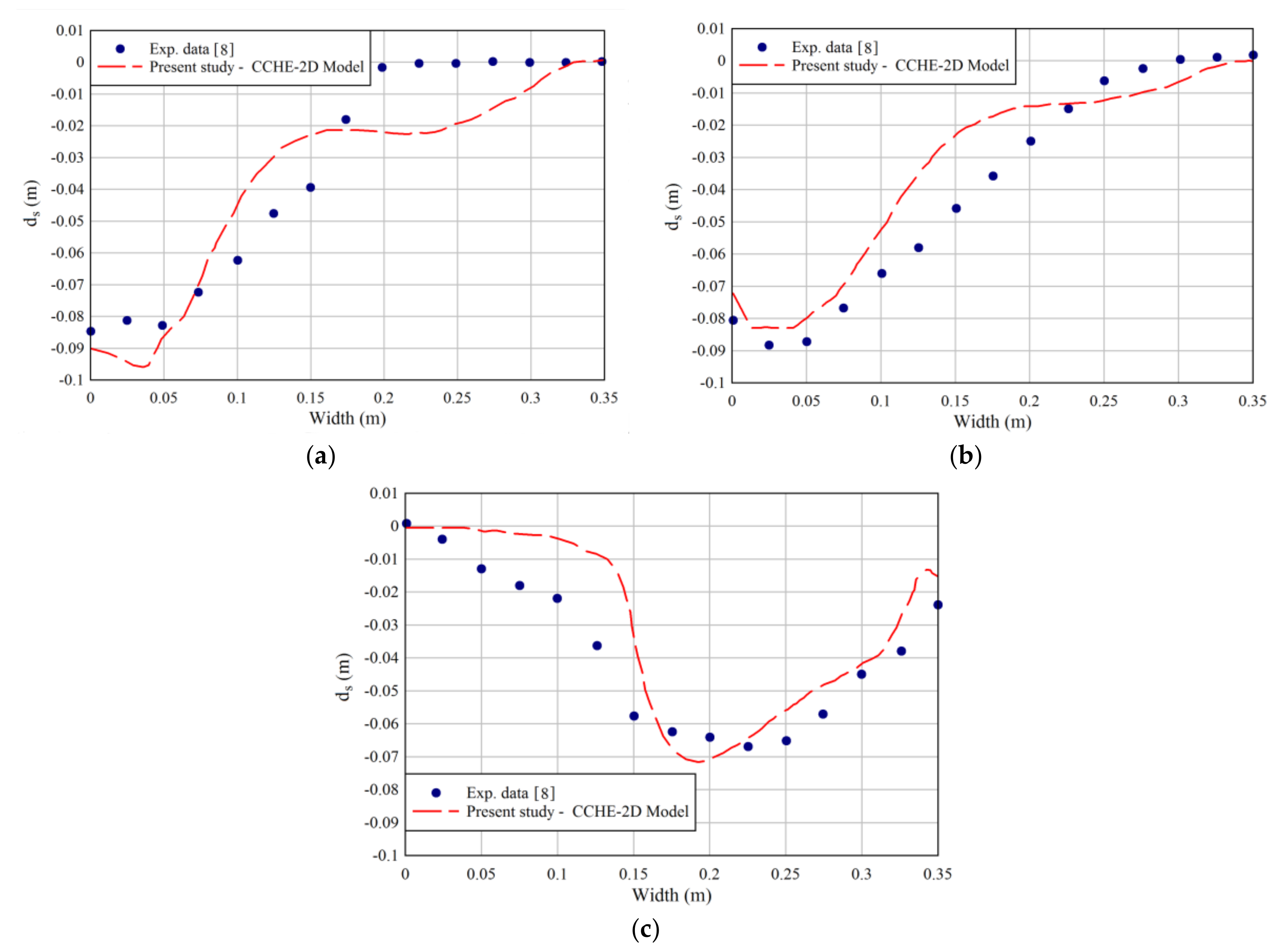
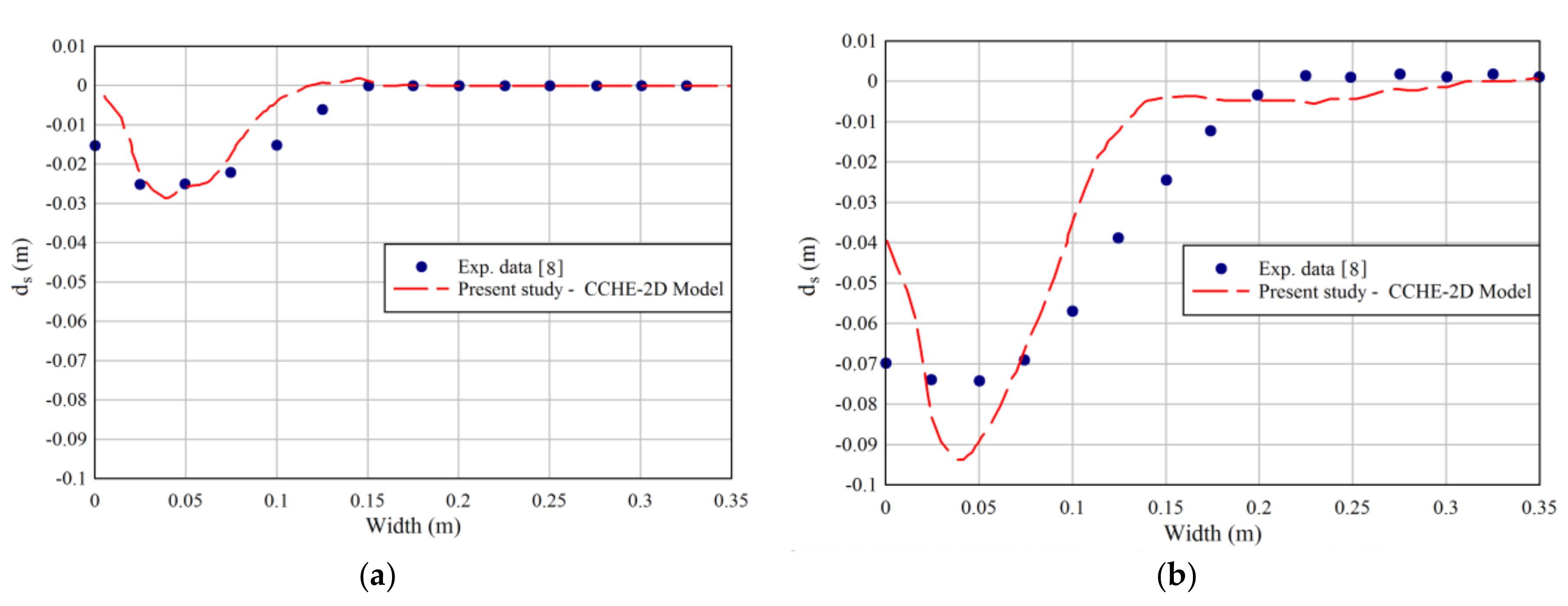
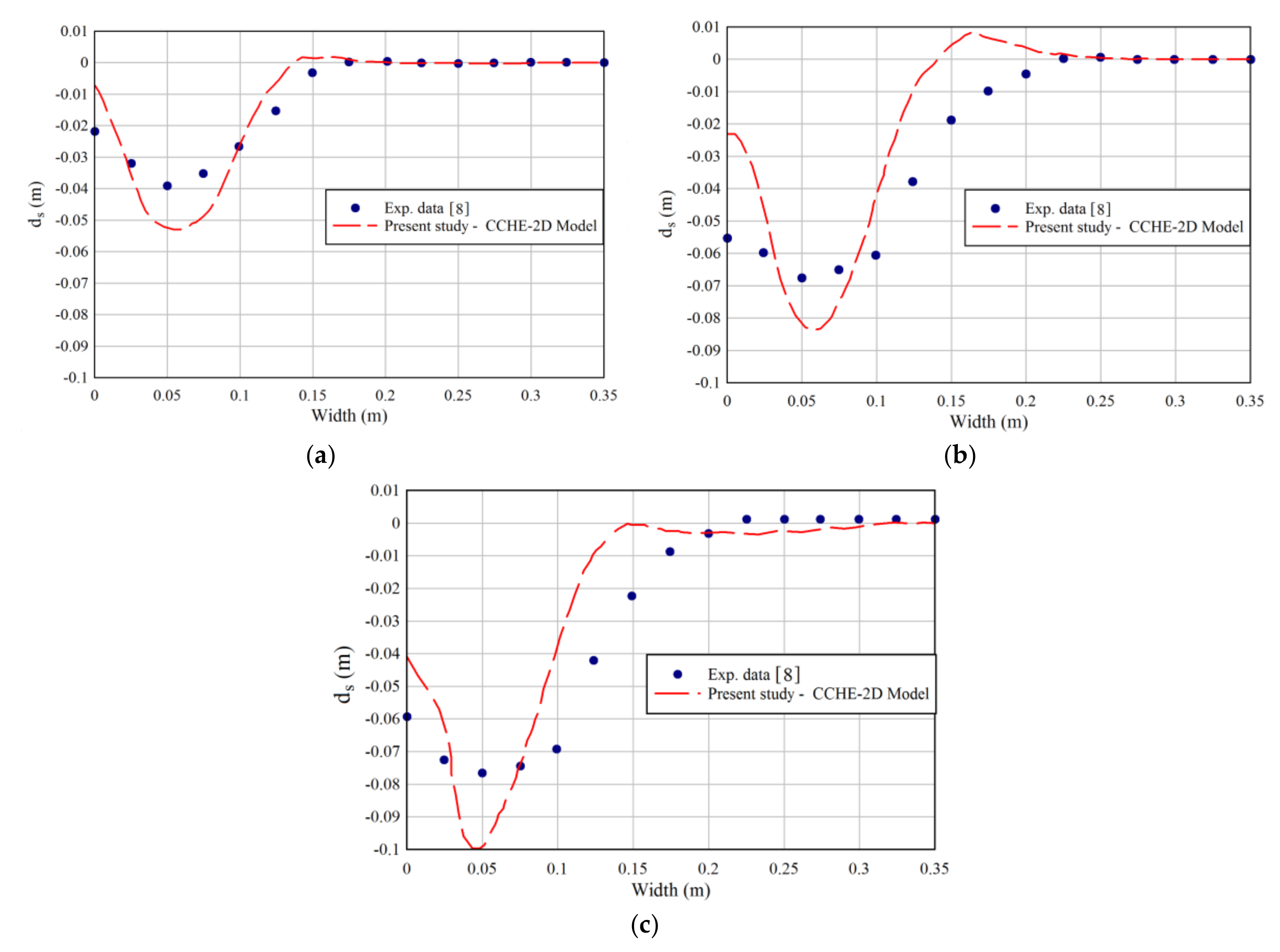
3.1. Model Verification

To achieve the desired objectives of this study, the results of the numerical modeling must be verified. To do this, simulation results were compared with the experimental results. Table 3 lists the simulations carried out for model verification. It should be mentioned that all comparisons were made for the width of 0.714 and the two flow rate ratios of 0.5 and 0.66 in accordance with the scenarios in Table 2.

Table 3. Simulations carried out for a comparison with the physical model.

Run	Downstream Flow Depth h3 (m)	Discharge Ratio Qr = (Q2/Q3)	Channel Width Ratio Br = (B2/B3)	Junction Angle θ (°)
1	0.13	0.5	0.714	90
2	0.155	0.66	0.714	90
4	0.155	0.5	0.714	90
5	0.155	0.5	0.714	75
6	0.11	0.66	0.714	75
7	0.13	0.5	0.714	60
8	0.13	0.66	0.714	60
9	0.1	0.5	0.714	60

Figure 6, Figure 7 and Figure 8 show a comparison between numerical results and experimental data for the transverse profiles of the bed in Section 1.

Figure 6. Comparison between experimental data and numerical results (θ = 90°). (a) Run 1; (b) Run 3; (c) Run 2.

Figure 7. Comparison between experimental data and numerical results (θ = 75°). (a) Run 5; (b) Run 6.

Figure 8. Comparison between experimental data and numerical results (θ = 60°). (a) Run 7; (b) Run 8; (c) Run 9.

Based on Figure 6, Figure 7 and Figure 8, it was observed that the left half of the transverse profiles of the eroded platform was placed in front of the entrance sub-channels. The exception was for junction angle of 90° with Q_r = 0.66 which scouring shifted to the right side of the channel due to the junction angle and discharge ratio. It was understood that the CCHE2D two-dimensional model with an acceptable accuracy was able to simulate the erosion distribution. The slope of scour hole in numerical modeling and measured values are close to each other with a reasonable accuracy, in other words.

Aimed at a junction angle between 60° to 70° in a field study on Rio Negro and Rio Solimões, Gualtieri et al. [19] observed that the maximum scouring area was on the right half of the cross-section immediately downstream of the Solimões mouth. Used for the confluence angle of 90°, the maximum scour depth was similar to the measured result. Quantitatively, at a confluence angle of 90°, the difference between the experimental and numerical maximum scour depth was approximately 8.5%. However, at confluence angles of 75° and 60°, this difference was 14% and 16%, respectively. Generally, it was seen that the eroded profile of the bed had an appropriate pattern and a similar trend. Based on the analyses, the average differences between the measured data and the simulation results for the flow ratios of 0.5 and 0.66 in all downstream depths were about 8% and 10.5%, respectively. The main reason for this difference is that the CCHE2D code uses a depth-averaged approach with no possibility of estimating the pressure and shear stress changes with full accuracy for the separation area.

3.2. Generalizing the Results to Other Cases

According to what was described in the previous section, several other runs were carried out in this study. They were done using a junction angle between 20° and 135°, the discharge ratios Q_r of 0.33, 0.55 and 0.66 and width ratios B_r of 0.428, 0.585, 0.714, 0.857, 1 and 1.142. Due to the abundance of runs, only one example is shown below. Table 4 lists all parameters regarding the range of variation for the numerical simulation. Figure 9 shows the flow depth contours for Run 2; the discharge ratio of 0.66, the width ratio of 0.714, and the confluence angle of 90°.

Table 4. Considered parameters and their range of variation in the numerical simulations.

Parameter	Range of Values
Width ratio Br	0.428, 0.585, 0.714, 0.857, 1.0 and 1.142
Discharge ratio Qr	0.33, 0.55 and 0.66
Junction angle θ	45, 60, 75, 90, 105, 120 and 135

Figure 9. Variation in water depth; Run 2.

Based on the flow zones described by Best [2] and Figure 9, in the main channel from the left side toward the opposite bank of the stream, the water depth decreased. Additionally, the shallow section was in the separation zone. The flow entrance from the tributary to the main channel and the interface with main channel flow resulted in a deviation of velocity vectors in the main channel toward its left bank (deflection zone), as shown in Figure 9. The same condition was observed in a field study about the Rio Negro and Rio Solimões confluence [35,36]. It is worth saying that anything that reduces the confluence-section downstream of the confluence of channels (including the backward area) could lead to an increase in upstream water depth. Figure 10 shows the distribution of flow velocity vectors for Run 2.

Figure 10. Distribution of depth averaged velocity for Run 2.

Figure 10 shows a separation zone occurred immediately downstream of the tributary mouth and the maximum flow rate was established in the mid-channel. The longitudinal velocity of flow was greatly reduced, and backward flow occurred in the separation zone; hence, in this section, horizontal vortexes were formed leading to sedimentation. Moreover, the transfer of momentum to the middle of the main channel and even to the opposite bank increased the shear stress in bed and caused sediment transport. Thus, it was expected that the maximum scour occurred in the opposite bank of the junction and the maximum deposition occurred in the downstream junction. Generally, according to the results, the shallow area was located just immediately downstream of the tributary mouth, in the separation zone. As the discharge ratio increased, the area of this region increased because the major flow moved to the right bank. This is quantitatively represented for all the simulated width ratios at the junction angle of 90° in Figure 11.

Figure 11. Q_r vs. h₁/h₃ for different B_r.

The above Figure shows the x-axis is the discharge ratio, Q_r, and the y-axis is the ratio of upstream depth to the downstream depth, h₁/h₃. Figure 10 shows an increase in the discharge ratio led to an increase in h₁/h₃. The reason is the difference in hydrostatic pressure. Since any increase in the discharge ratio resulted in an increasing separation zone, the conversion of dynamic pressure to static pressure happened in a wider area. This, in turn, caused a bigger difference in the static pressure between the upstream and the downstream of the confluence. Quantitatively, the change of discharge ratio Q_r from 0.33 to 0.66 on average led to a 7% and 4% increase in relative depth for the width ratios of 0.428 and 1.142, respectively. This means that the effect of discharge ratio for smaller width ratios was greater. The same analysis could be done to investigate the effect of the junction angle. Figure 12 shows the effect of junction angle θ on the ratio of water depth h₁/h₃.

Figure 12. Q_r vs. h₁/h₃ for different θ.

Figure 12 presents the averaged numerical results for all width ratios. Obviously, by increasing the junction angle, the relative depth increased. The reason can be explained in the context of the increased static pressure. Quantitatively, the angle of 45° did not have a significant impact on the increase of the relative flow depth, because it was added in parallel to flow lines in the main channel and had the lowest pressure difference. As the discharge increased from 0.33 to 0.66 at the junction angle of 135°, the relative depth increased approximately 6%. Generally, the ratio of the depth of the main channel to the tributary channel at the confluence was always greater than one. This is due to the significant energy losses at the entrance into the main channel and in flow separation; these energy losses were compensated by an increase in the flow depth. The ratio of h₁/h₃ increased with the increasing discharge ratio Q_r.

This trend was more pronounced in the discharge ratio of 0.66. However, as the width ratio B_r increased, the depth ratio h₁/h₃ decreased. As the width ratio decreased from 0.857 to 0.428, in terms of quantity, in discharge ratio Q_r of 0.66, the relative depth increased on average of about 2%. Figure 13 shows the effect of discharge ratio to the maximum depth of erosion.

Figure 13. Q_r vs. ds/B₃ for different B_r.

Figure 13 shows d_s was the maximum depth of scour and d_s/B₃ was the relative maximum scour depth. According to this Figure, which was plotted for θ = 90°, an increase in discharge ratio led, for all width ratios, to an increase in the relative scour depth.

A quantitative analysis of maximum scouring variations for different width ratios is listed in Table 5. Negative values and positive values mean, reduction and increase, respectively, in d_s/B₃ compared to a width ratio of 0.428.

Table 5. Change (%) of ds/B₃ for different widths as compared to Br = 0.428.

Br = 1.142	Br = 1.00	Br = 0.857	Br = 0.571	Br = 0.714	Qr
−72.22	−50.01	−22.22	16.67	94.44	0.33
−46.51	−39.53	−34.88	37.21	97.67	0.5
−60.23	−51.14	−35.23	19.32	30.68	0.66

Table 5 shows that an increasing width ratio generally led to a decrease in the maximum scour depth. Figure 14 presents the effects of discharge ratio on the maximum scouring depth for different junction angles θ.

Figure 14. Q_r vs. d_s/B₃ for different θ.

Figure 14 depicts that an increase in the junction angle generally resulted in an increase in the maximum relative scour depth. Table 6 lists the variation of the relative maximum depth as compared to a junction angle of 90°.

Table 6. Change (%) of D_s/B₃ for different θ as compared to θ = 90°.

θ = 135°	θ = 120°	θ = 105°	θ = 75°	θ = 60°	θ = 45°	Qr
105.56	61.11	33.35	−33.34	−55.56	−72.22	0.33
79.07	16.28	9.37	−9.31	−27.91	−41.86	0.5
39.78	14.77	5.68	−7.95	−20.45	−35.23	0.66

According to Table 6, an increase in discharge ratio for any junction angle decreased the maximum scour depth. The numerical results of this study can be compared with the results from Habibi et al. [37] for this parameter. They simulated with the CCHE2D code a model with the main channel width of 0.5 m, the tributary channel width of 0.15 m, and the junction angle of 90°. Width ratio was 0.3. Three discharge ratios of 0.11, 0.15 and 0.23 were investigated. Table 7 lists a comparison between the present numerical results and those from Habibi et al. [37]. The location of the mixing interface depends on the momentum ratio and the angular orientation of the two tributary channels with respect to alignment of the downstream channel. Changes in these factors resulted in a lateral shift in the position of the mixing interface across the confluence, as well as results presented by Baluchi et al. (2015) [38] and Baghlani and Talebbeydokhti [39]. Table 7 shows an acceptable agreement between both studies. Furthermore, by increasing the discharge ratio, the dimensionless rate of maximum scouring depth increased in both studies.

Table 7. Comparison between the current study and the results from Habibi et al. [37].

Habibi et al. [37]		Present Study for Br = 0.428 and θ = 90°
Qr	ds/B3	Qr	ds/B3
0.11	0.0143	0.33	0.1
0.15	0.0024	0.5	0.243
0.23	0.0352	0.66	0.328

4. Conclusions

The CCHE2D code was used to analyze the flow and erosion patterns at a laboratory confluence. Moreover, the effects of each of the influential parameters including the discharge ratio, the ratio of the width and the angle of the confluence on relative depth and maximum scouring depth were studied. First, the calibration of the model was done based upon a Manning coefficient so that different Manning’s n were analyzed, then, for model verification, the results were compared with literature experimental data. The main conclusions are:

• Though the morphodynamic and hydrodynamic processes are complicated regarding the confluence zone, in most cases, the transverse profile of bed level had an acceptable agreement between numerical and measured results.
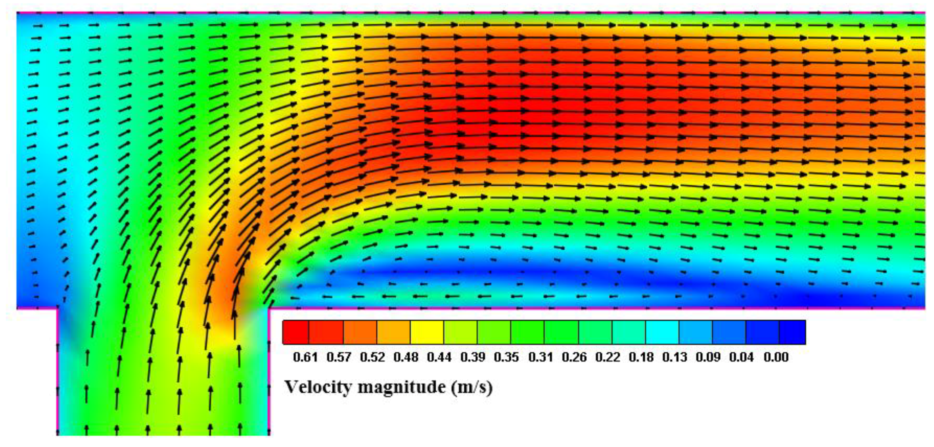
• The separation zone was precisely simulated. Therefore, the results showed that the increasing angle of junction θ resulted in an increasing width of the separation zone. Moreover, by reducing B_r, the size (length and width) of the separation zone increased. Conversely, with an increase in the width ratio, the maximum depth of bed erosion decreased. By increasing the junction angle θ, the maximum depth of bed erosion at the confluence increased.
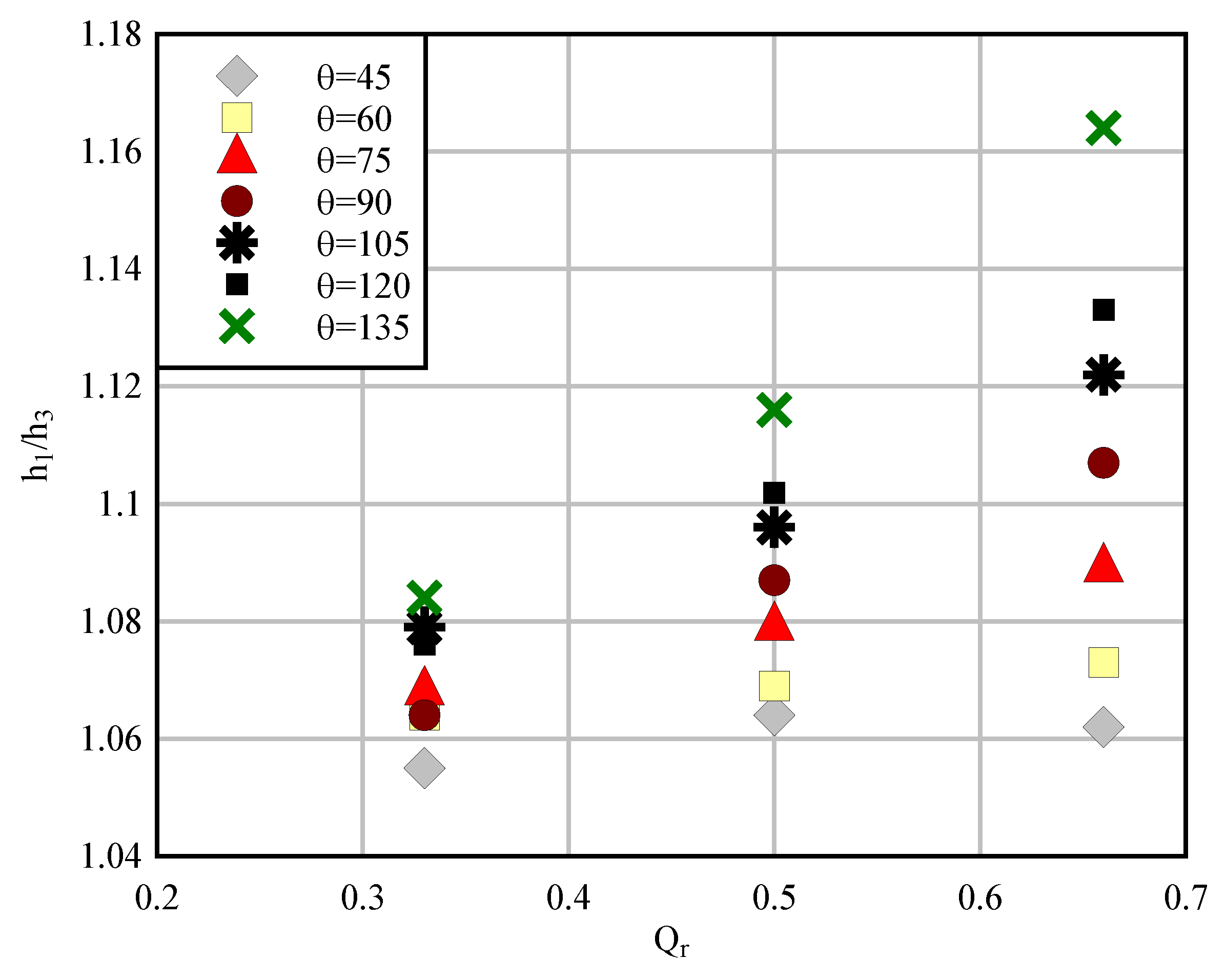
• The relative depth of the main channel flow to the tailwater depth, in terms of quantity, h₁/h₃ was always greater than one. An increase in the discharge ratio Q_r resulted in the ratio h₁/h₃ having an increasing trend that was more evident for Q_r = 0.66. Moreover, by increasing the width ratio, the depth ratio of the main channel to tailwater decreased.
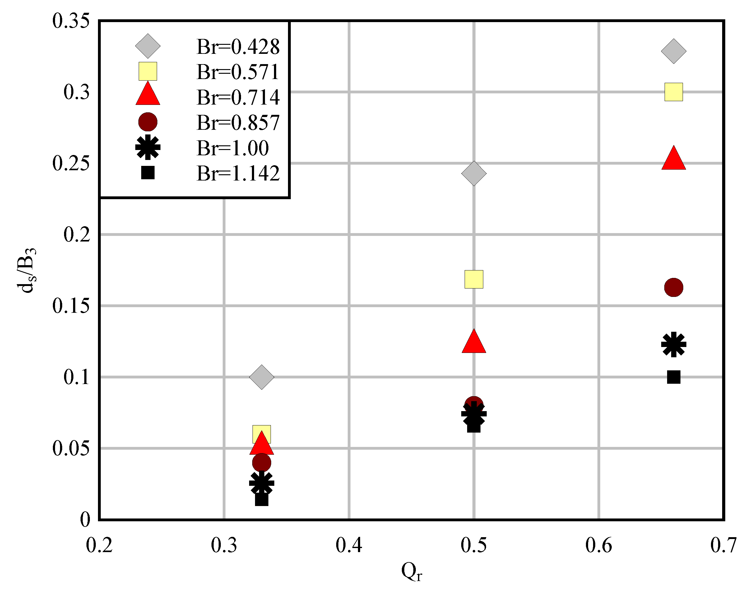
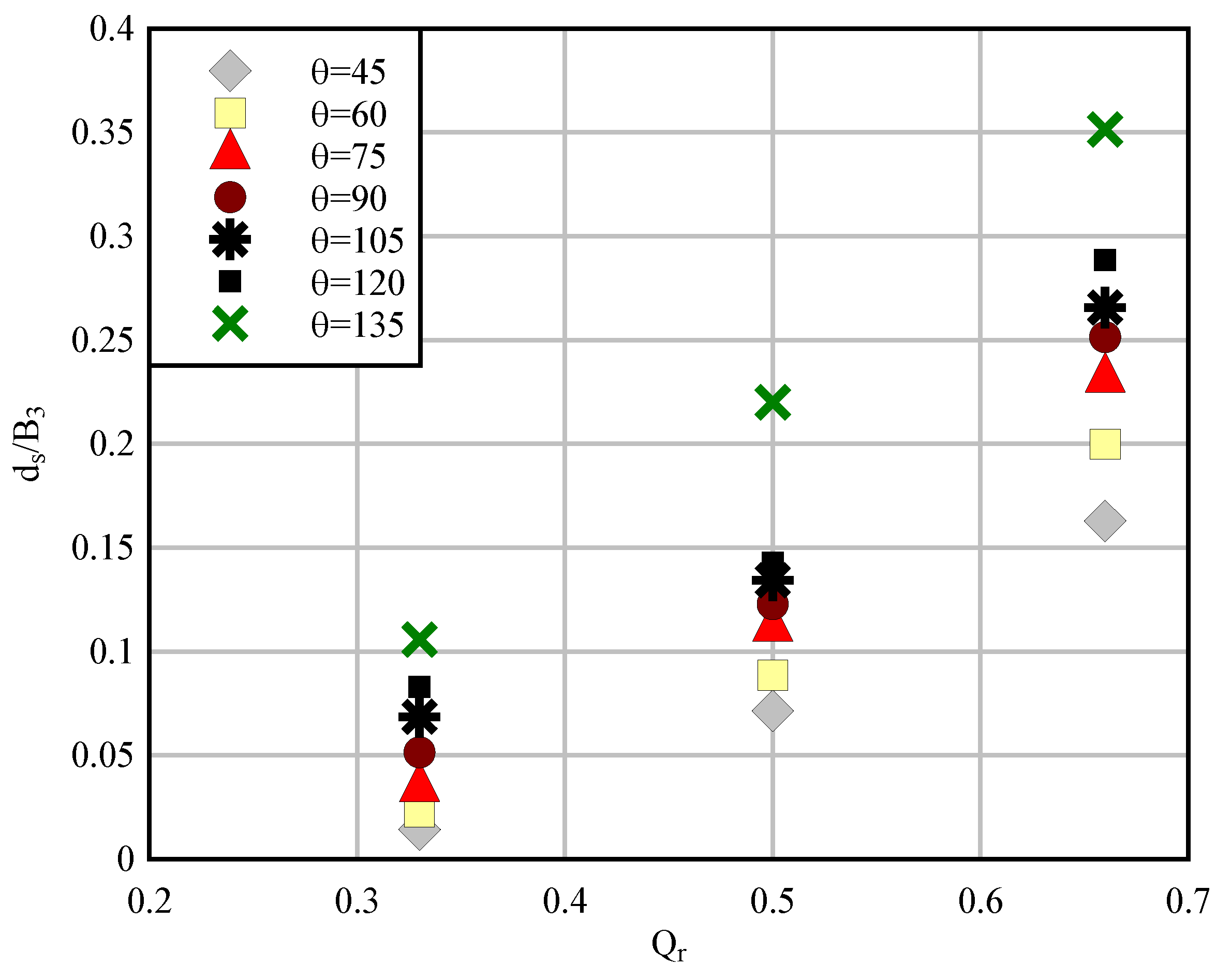
• The maximum relative scour depth d_s/B₃ was studied for different angles of junction, width ratio, and discharge ratio. An increase in discharge ratio led to an increase in d_s/B₃ for all width ratios; increasing width ratio generally led to a decrease in d_s/B₃ and an increase in the junction angle generally resulted in an increase in d_s/B₃. Furthermore, comparisons with other studies confirmed an acceptable agreement between them.

The results presented in this study demonstrated that CCHE2D model can be applied for simulating the flow and scouring at a laboratory confluence with acceptable accuracy. Future studies will be addressed to try to extend this capabilities to larger scale confluences.

References

- Kenworthy, S.; Rhoads, B. Hydrologic control of spatial patterns of suspended sediment concentration at a stream confluence. J. Hydrol. 1995, 168, 251–263. [Google Scholar] [CrossRef]
- Best, J.L. Sediment transport and bed morphology at river channel confluences. Sedimentology 1988, 35, 481–498. [Google Scholar] [CrossRef]
- Trevethan, M.; Santos, R.V.; Ianniruberto, M.; Poitrasson, F.; Gualtieri, C. Observations of hydrodynamics and water chemistry about the confluence of Rio Negro and Rio Solimões. In Proceedings of the XV Brazilian Geochemistry Congress, Brasilia, Brazil, 19–22 October 2015. [Google Scholar]
- Biron, P.; Lane, S. Modelling hydraulics and sediment transport at river confluences. In River Confluences, Tributaries and the Fluvial Network; Rice, S., Roy, A., Rhoads, B., Eds.; John Wiley & Sons: Hoboken, NJ, USA, 2008; pp. 17–43. [Google Scholar]
- Best, J.L.; Rhoads, B.L. Sediment transport, bed morphology and the sedimentology of river channel confluences. In River Confluences, Tributaries and the Fluvial Network; Rice, S., Roy, A., Rhoads, B., Eds.; John Wiley & Sons: Hoboken, NJ, USA, 2008; pp. 45–72. [Google Scholar]
- Rhoads, B.; Sukhodolov, A. Lateral momentum flux and the spatial evolution of flow within a confluence mixing interface. J. Water Resour. Res. 2008, 22, W08440. [Google Scholar] [CrossRef]
- Bryan, R.B.; Kuhn, N.J. Hydraulic condition in experimental rill confluences and scour in erodible soils. J. Water Resour. Res. 2002, 38, 1–22. [Google Scholar] [CrossRef]
- Ghobadian, R. Experimental Study of Flow and Sediment Pattern at River Confluence. Ph.D. Thesis, Shahid Chamran University, Ahvaz, Iran, September 2006. [Google Scholar]
- Lane, S.; Parsons, D.; Best, J.; Orfeo, O.; Kostaschunk, R.; Hardy, R. Causes of rapid mixing at a junction of two large rivers: Rio Parana and Rio Paraguay, Argentina. J. Geophys. Res. 2008, 113, F02019. [Google Scholar] [CrossRef]
- Leite Ribeiro, M.; Blanckaert, K.; Roy, A.G.; Schleiss, A.J. Flow and sediment dynamics in channel confluences. J. Geophys. Res. 2012, 117. [Google Scholar] [CrossRef]
- Đorđević, D. Application of 3D numerical models in confluence hydrodynamics modelling. In Proceedings of the XIX International Conference on Water Resources, Urbana, IL, USA, 17–21 June 2012. [Google Scholar]
- Yang, Q.; Liu, T.; Lu, W.; Wang, X. Numerical simulation of confluence flow in open channel with dynamic meshes techniques. Adv. Mech. Eng. 2013, 5, 1–10. [Google Scholar] [CrossRef]
- Constantinescu, G.; Miyawaki, S.; Rhoads, B.; Sukhodolov, A. Numerical evaluation of the effects of planform geometry and inflow conditions on flow, turbulence structure, and bed shear velocity at a stream confluence with a concordant bed. J. Geophys. Res. Earth Surf. 2014, 119, 2079–2097. [Google Scholar] [CrossRef]
- Mignot, E.; Vinkovic, I.; Doppler, D.; Riviere, N. Mixing layer in open-channel junction flows. Environ. Fluid Mech. 2014, 14, 1027–1041. [Google Scholar] [CrossRef]
- Schindfessel, L.; Creëlle, S.; De Mulder, T. Flow Patterns in an Open Channel Confluence with Increasingly Dominant Tributary Inflow. Water 2015, 7, 4724–4751. [Google Scholar] [CrossRef]
- Guillén-Ludeña, S.; Franca, M.J.; Alegria, F.; Schleiss, A.J.; Cardoso, A.H. Hydromorphodynamic effects of the width ratio and local tributary widening on discordant confluences. Geomorphology 2017, 293, 289–304. [Google Scholar] [CrossRef]
- Gualtieri, C.; Filizola, N.; Olivera, M.; Santos, A.M.; Ianniruberto, M. A field study of the confluence between Negro and Solimões Rivers. Part 1: Hydrodynamics and sediment transport. Comptes Rendus Geosci. 2018, 350, 31–42. [Google Scholar] [CrossRef]
- Gualtieri, C.; Ianniruberto, M.; Filizola, N.; Santos, R.; Endreny, T. Hydraulic complexity at a large river confluence in the Amazon basin. Ecohydrology 2017, 10. [Google Scholar] [CrossRef]
- Bradbrook, K.F.; Lane, S.N.; Richards, K.S. Numerical simulation of three-dimensional, time-averaged flow structure at river channel confluences. Water Resour. Res. 2000, 36, 2731–2746. [Google Scholar] [CrossRef]
- Shakibainia, A.; Majdzadeh Tabatabai, M.R.; Zarrati, A.R. Three-dimensional numerical study of flow structure in channel confluences. Can. J. Civ. Eng. 2010, 37, 772–781. [Google Scholar] [CrossRef]
- Ramamurthy, A.S.; Qu, J.; Zhai, C. 3D simulation of combining flows in 90 rectangular closed conduits. J. Hydraul. Eng. 2006, 2, 214–218. [Google Scholar] [CrossRef]
- Bahmanpouri, F.; Filizola, N.; Ianniruberto, M.; Gualtieri, C. A new methodology for presenting hydrodynamics data from a large river confluence. In Proceedings of the 37th IAHR World Congress, Kuala Lumpur, Malaysia, 13−18 August 2017. [Google Scholar]
- Fathi, M.; Honarbakhsh, A.; Rostami, M.; Nasri, M.; Moradi, Y. Sensitive analysis of calculated mesh for CCHE2D numerical model. World Appl. Sci. J. 2012, 18, 1037–1051. [Google Scholar]
- Chao, X.; Jia, Y.; Wang, S.S.Y.; Azad Hossein, A.K.M. Numerical modeling of surface flow and transport phenomena with applications to Lake Pontchartrain. Lake Reserv. Manag. 2012, 28. [Google Scholar] [CrossRef]
- Duan, J.G.; Wang, S.S.Y.; Jia, Y. The applications of the enhanced CCHE2D model to study the alluvial channel migration processes. J. Hydraul. Res. 2001, 39, 469–480. [Google Scholar] [CrossRef]
- Nguyen, V.T.; Moreno, C.S.; Lyu, S. Numerical simulation of sediment transport and bed morphology around Gangjeong Weir on Nakdong River. KSCE J. Civ. Eng. 2015, 19, 2291–2297. [Google Scholar] [CrossRef]
- Pu, J.H. Turbulence Modelling of Shallow Water Flows using Kolmogorov Approach. Comput. Fluids 2015, 115, 66–74. [Google Scholar] [CrossRef]
- Zhang, Y. CCHE2D-GUI—Graphical User Interface for the CCHE2D Model, User’s Manual—Version 2.0; National Center for Computational Hydroscience and Engineering: Oxford, MS, USA, 2003. [Google Scholar]
- Pu, J.H.; Bakenov, Z.; Adair, D. Assessment of a shallow water model using a linear turbulence model for obstruction-induced discontinuous flows. Eurasian Chem. Technol. J. 2012, 14, 155–167. [Google Scholar] [CrossRef]
- Erpicum, S.; Meile, T.; Dewals, B.J.; Pirotton, M.; Schleiss, A.J. 2D numerical flow modeling in a macro-rough channel. Int. J. Numer. Meth. Fluids 2009, 61, 1227–1246. [Google Scholar] [CrossRef]
- Blocken, B.; Gualtieri, C. Ten iterative steps for model development and evaluation applied to Computational Fluid Dynamics for Environmental Fluid Mechanics. Environ. Model. Softw. 2012, 33, 1–22. [Google Scholar] [CrossRef]
- Wu, W.; Wang, S.S.Y. Movable bed roughness in alluvial rivers. J. Hydraul. Eng. 1999, 125, 1309–1312. [Google Scholar] [CrossRef]
- Van Rijn, L.C. Sediment transport, part III: Bed forms and alluvial roughness. J. Hydraul. Eng. 1984, 110, 1733–1754. [Google Scholar] [CrossRef]
- Pu, J.H.; Hussain, K.; Shao, S.; Huang, Y. Shallow Sediment Transport Flow Computation Using Time-Varying Sediment Adaptation Length. Int. J. Sediment Res. 2014, 29, 171–183. [Google Scholar] [CrossRef]
- Trevethan, M.; Martinelli, A.; Oliveira, M.; Ianniruberto, M.; Gualtieri, C. Fluid dynamics, sediment transport and mixing about the confluence of Negro and Solimões rivers, Manaus, Brazil. In Proceedings of the 36th IAHR World Congress, The Hague, The Netherlands, 28 June 28–3 July 2015. [Google Scholar]
- Trevethan, M.; Ventura Santos, R.; Ianniruberto, M.; Santos, A.; De Oliveira, M.; Gualtieri, C. Influence of tributary water chemistry on hydrodynamics and fish biogeography about the confluence of Negro and Solimões rivers, Brazil. In Proceedings of the 11th International Symposium on EcoHydraulics, Melbourne, Australia, 2–7 February 2016. [Google Scholar]
- Habibi, S.; Rostami, M.; Musavi, A. Numerical Investigation of flow patterns and sediment at the confluence of the rivers. Iran. J. Watershed Manag. Sci. Eng. 2014, 8, 19–29. [Google Scholar]
- Balouchi, B.; Nikoo, M.R.; Adamowski, J. Development of expert systems for the prediction of scour depth under live-bed conditions at river confluences: Application of different types of ANNs and the M5P model tree. Appl. Soft Comput. J. 2015, 34, 51–59. [Google Scholar] [CrossRef]
- Baghlani, A.; Talebbeydokhti, N. Hydrodynamics of right-angled channel confluences by a 2D numerical model. Iran. J. Sci. Technol. 2013, 37, 271–283. [Google Scholar]
© 2018 by the authors. Licensee MDPI, Basel, Switzerland. This article is an open access article distributed under the terms and conditions of the Creative Commons Attribution (CC BY) license (http://creativecommons.org/licenses/by/4.0/).