Abstract
Estimating economic losses caused on buildings and other civil engineering works due to flooding events is often a difficult task. The accuracy of the estimate is affected by the availability of detailed data regarding the return period of the flooding event, vulnerability of exposed assets, and type of economy run in the affected area. This paper aims to provide a quantitative methodology for the assessment of economic losses associated with flood scenarios. The proposed methodology was performed for an urban area in Southern Italy prone to hydrogeological instabilities. At first, the main physical characteristics of the area such as rainfall, land use, permeability, roughness, and slopes of the area under investigation were estimated in order to obtain input for flooding simulations. Afterwards, the analysis focused on the spatial variability incidence of the rainfall parameters in flood events. The hydraulic modeling provided different flood hazard scenarios. The risk curve obtained by plotting economic consequences vs. the return period for each hazard scenario can be a useful tool for local authorities to identify adequate risk mitigation measures and therefore prioritize the economic resources necessary for the implementation of such mitigation measures.
1. Introduction
Flooding events can affect the lives of many communities, especially by damaging their assets. According to records the frequency of such events is increasing worldwide, and flooding events often cause economic losses greater than other natural disasters [1]. Although the death toll is relatively stable across all flooding events, the related economic losses are rising worldwide [2]. Moreover, the anthropic impact on land use changes can exacerbate the effects of floods, especially at the local scale [3]. Therefore, techniques based on Geographical Information System (GIS) and Remote Sensing Imagery (RSI) have recently been adopted for the analysis of river basin behavior during flooding events in order to improve the extraction of land use factors [4].
The economic losses due to hydrological events, i.e., floods and mass movements constituted by soil and debris, was estimated to be around EUR 165 billion (in 2015 EUR values) among all EU member countries over the period of 1980–2015. This estimate represents one-third of the total economic losses due to natural disasters for all EU member countries [5].
The assessment of potential negative effects in flooding areas affected by anthropic modification can be achieved by a risk estimation of these hybrid systems in order to obtain an accurate and objective assessment of the threat level related to potential hazardous phenomena [6,7]. As a matter of fact, the production of flood risk maps is a crucial task to identify and schedule structural and non-structural mitigation measures in a proactive way, reducing the potential negative impacts due to the occurrence of hazardous hydrological events. Risk assessment takes into account “the geographic coverage of the hazard, the exposure of people, property, and infrastructure to the hazard, and the vulnerability of people, property, and infrastructure to the event and impact” [8]. However, flood maps must be related to socioeconomic factors to assess the potential impact on communities and their assets [8]. Moreover, the economic damage assessment related to a generic natural and technological calamity can support decision-making at different spatial scales, especially as regards the adaptation to climatic changes [9].
A distinction must be made related to flood damage typologies. Damages immediately consequent to the impact of floodwaters are called direct, whereas those following the impact are defined as indirect damages. Moreover, damages are classified as tangible if the damages can be quantified in monetary values; otherwise, they are classified as intangible [10,11].
Estimating economic losses caused to buildings and other civil engineering works due to flooding events is often a difficult task. The accuracy of the estimate is affected by the availability of detailed data regarding the return period of the flooding event, vulnerability of exposed assets, and type of economy run in the affected area. In addition, interconnections between physical and social vulnerabilities increase the complexity of the estimate even further at different time and spatial scales, [12]. This can cause cascading effects, which amplify the negative consequences related to the trigger event [13].
The economic evaluation of tangible damages is often referred to a national or regional scale. The literature offers many methodologies to assess the economic impact of potential flooding concerning direct losses [10] or both direct and indirect losses [2]. This may be due to the extent of the territory considered in the planning activity, i.e., national or regional, and the lack of detailed and classified data at the local scale [9].
In the light of the above, this work aims to provide a quantitative assessment of risk exposure to flood events and economic risk of flood events at the local scale. This methodology concerns tangible and direct losses related to flood scenarios and attempts to quantify the economic losses consequent to potential flood events with different return periods. In order to obtain the economic consequences for each return period, firstly the economic value of the elements at risk were estimated by multiplying the unit market values or unit construction costs with the quantity of exposed elements for the considered return period across several categories of different exposed elements [14]. Secondly, the economic value of the elements at risk was multiplied by the percentage of damage associated with each element at risk. This was obtained by means of flood damage functions which relate the damage of each element at risk with flood water levels and flow velocities [15,16]. Lastly, an estimation of the total risk was derived by plotting the return period values against the quantified exposure to determine the risk curve [17]. Furthermore, the quantitative assessment of economic risk for each sub-basin of the area under investigation was carried out to identify the areas susceptible to direct damages due to potential flood events at the local scale. The proposed approach complies with the provisions issued by the European Parliament Directive 2007/60/EC on 23 October 2007 concerning the assessment and management of flood risks [18].
The basin including the urban area of San Giovanni Rotondo (Gargano area, Apulia region, Southern Italy) was chosen to test the methodology proposed in this paper. This area is periodically affected by flood events characterized by debris transport, as are many other areas in the surrounding region. As a matter of fact, San Giovanni Rotondo was one of the urban settlements most affected by a period of heavy rainfalls in 2014, with consequent several damages to buildings and transport systems [19]. Finally, the limitations of this methodology and potential future implementations are described to enable a holistic economic assessment of flood risk at the local scale.
2. The Study Area
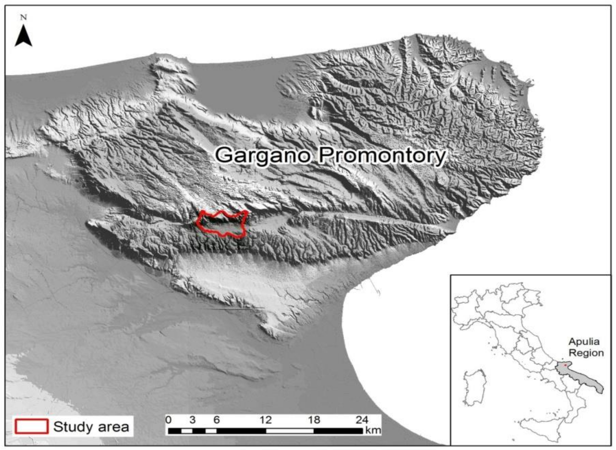
The study area covers the urban center of San Giovanni Rotondo (Apulia Region, Southern Italy—Figure 1), which is the most populous municipality of Gargano, home to more than 27,000 inhabitants.

Figure 1.
Study area.
The inhabited center is included in an endorheic basin with obvious signs of karst engravings such as depressions and sinkholes. From a geostructural point of view, the Gargano promontory belongs to the Apulia Foreland and it is characterized by a litostratigraphic succession more than 4000 m deep and composed of Meso-Cenozoic carbonatic rocks [20,21]. The entire promontory, consisting in an anticlinal towards WNW-ESE, is affected by several faults. The morphology of the Gargano area is the result of tectonic processes that have generated a succession of reliefs and depressions. In particular, the urban area of San Giovanni Rotondo is located in a depressed plain surmounted by a steep hillslope in the north that is characterized by limestones, dolomitic limestones, and dolomite outcrops. The basin area under investigation is circa 15 km2. Maximum and minimum elevations are 1006 m and 540 m, respectively, with an average height of the basin of 684 m. The average slope is about 10.44% with a maximum peak of around 66%. The climate has an average temperature of 13.8 °C with an average annual total rainfall of 844 mm [22].
The study area suffers periodic flood events which trigger debris flows along the northern hillslope of the basin. The Gargano area, due to the lithological and structural features of outcropping lithologies (generally limestones), is mostly affected by rockfalls. During flood events, the detrital superficial strata covering the northern hillslope of the basin are diluted by the remarkable water amount channeled in the basin, generating debris flows. This type of slope instability mechanism is less widespread and different from the landslides that notoriously affect the area to the west of Gargano, known as Daunian Subappennine, located in the Apulia region about 50 km from the study area. The slope instability mechanisms in this area farther from the study area consist of composite and complex landslides, ranging in type, volume, and velocity, from deep slow roto-translational slides to shallow moderately fast earthflows [23], and affect the clayey succession of the Apenninic Chain [24]. Nevertheless, the northern rocky hillslope overhanging the urban center is considered susceptible to slope instability by the River Basin Authority of Apulia Region; however, as this instability is strictly associated with and triggered by flood events, landslides are not considered a risk factor in this study.
In particular, from 1 to 6 September 2014, the study area was affected by a strong meteorological event that caused floods and heavy damage throughout the whole Gargano [19]. The most affected zones were those of recent development in the depressed areas of the basin. This area has cultural, social, and economic importance due to the presence of a sanctuary and a hospital, known at the regional and national level. Indeed, in last years, the area has become one of the major Italian cities for religious tourism, with hundreds of thousands of visitors coming from all over the world, as well as a point of reference for regional health.
3. Materials and Methods
3.1. Hydrologic Modeling
The first phase of the study focused on the hydrological analysis of the area. This allowed the evaluation of the hydrological discharge as input data of the two-dimensional hydraulic numerical model adopted in this work for the analysis of the hazard scenarios.
The maps of flood-prone areas were obtained after evaluating the peak flowrate for the three considered return periods. The rainfall Intensity-Duration-Frequency (IDF) curves were estimated by regional analysis of the annual maxima of rainfall intensity performed with a probabilistic model based on the use of a Two Component Extreme Value Distribution [25], Maximum Likelihood estimator, and hierarchical estimation of regional model parameters [26]. In particular, we used a regional analysis of the annual maximums of precipitation in the Apulia region [27].
To estimate the rainfall IDF, the following expression was adopted:
where:
- im is the average intensity of rain, a function of the duration of the rainfall event (t) and of the return period (TR);
- a is a parameter depending on the return period (TR);
- n is a parameter that defines the decrease of rainfall intensity over time.
The study analyzed three scenarios as follows:
- Scenario 1: TR = 30 years;
- Scenario 2: TR = 200 years;
- Scenario 3: TR = 500 years.
The Apulia Basin Authority (Autorità di Bacino, AdB) indicates the return period values chosen for each scenario for the definition of the three classes of hydraulic hazard (low, middle, and high), in accordance with the hydrogeological system plan called “Piano di Assetto Idrogeologico (PAI) Puglia” [28].
The calculation of the curve was performed through a probabilistic analysis of the annual maximum rainfall of assigned duration, using the VA.P.I. method provided by the National Group for the Defense from Hydrogeological Disasters [27] with “aims to set up a uniform procedure throughout the national territory for the evaluation of the natural flood discharge”.
In the Apulia region, the project is based on an exhaustive study [27]. Precisely, the territory of Apulia was divided into six homogeneous zones for rainfall through a “regionalization” process. Each zone has an equation that allows the associated IDF curve to be estimated, based on the rainfall height (expressed in mm). The basin examined is in zone 1, corresponding to the relationship:
where:
- h represents the height of rainfall (expressed in millimeters of precipitation);
- z is the mean elevation of the basin. In this case it is about 684 m.
Rainfall values must be modified using two coefficients. These are the Areal Reduction Factor (ARF) and the Growth Factor (KT). The former can be evaluated as follows:
- ARF is the ratio of the mean areal rainfall (hs) to the mean point rainfall (hp) in the same area. It is a function of time (t), basin area (A), and return period (TR);
- hs is the mean areal rainfall and is a function of time (t), basin area (A), and return period (TR);
- hp is the mean point rainfall and is a function of time (t) and return period (TR).
Studies conducted by the US Weather Bureau (1957–1960) [29,30,31,32,33,34] in the eastern United States and by Penta (1974) [35] in southern Italy have shown a negligible dependence on the return period. Therefore, an alternative approach to evaluate the ARF was proposed as follows:
In 1972, Eagleson [36] defined:
Penta [35] indicated values considered acceptable for southern Italy as follows:
C1 = 2.1 × 10⁻³; C2 = 0.53; C3 = 0.25.
Experimentally, KT is found to be constant for zones 1, 2, 3, and 4 in the Apulia region [27], and it can be evaluated by the following equation:
For the three considered return periods, values of corrected height of rainfall (hc) are obtained:
This variable is connected to the intensity of rainfall by the relationship:
Thus, the IDF curve can also be expressed, in terms of height of rainfall, as:
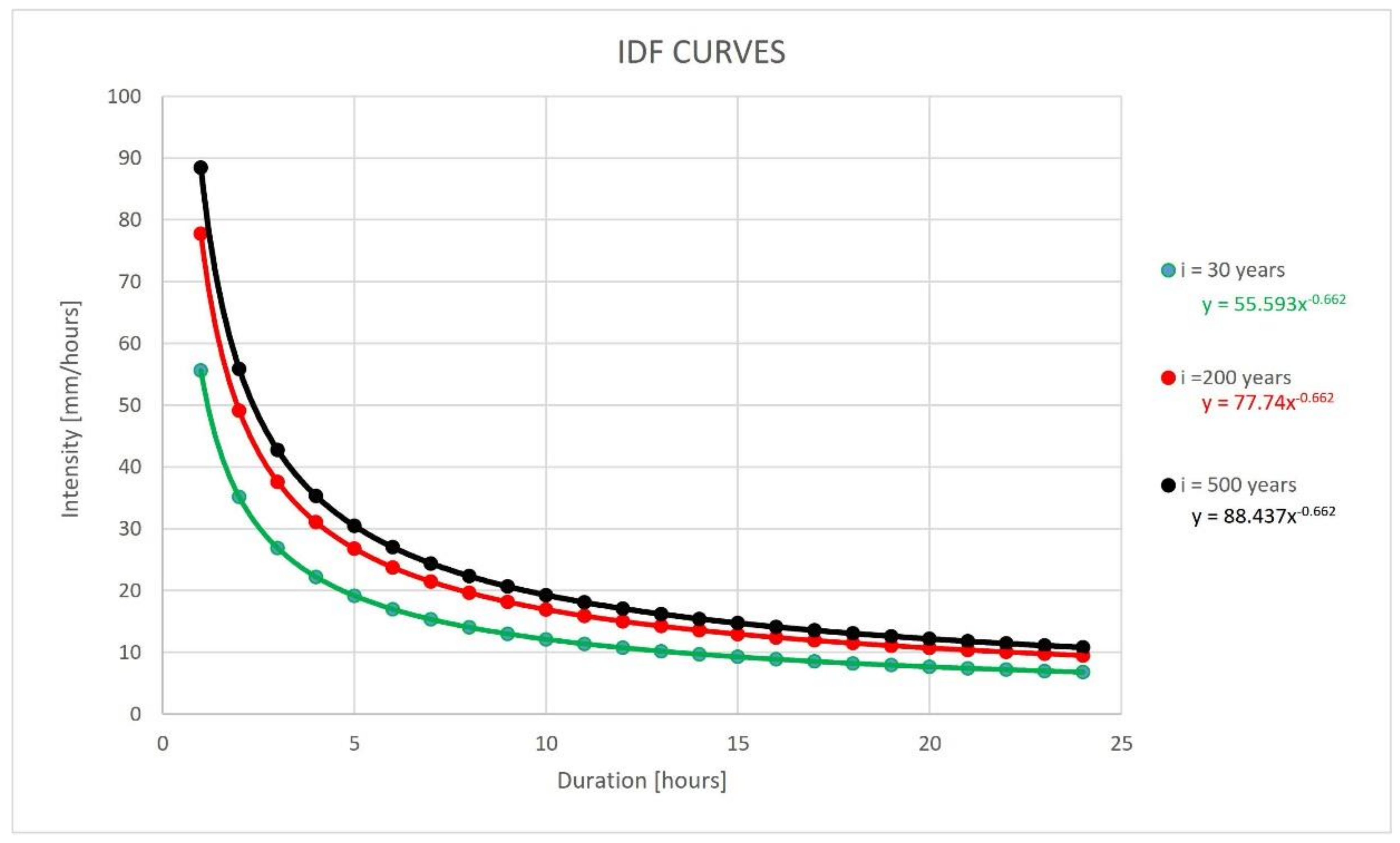
The results of the hydrological analysis for the three scenarios are shown in Figure 2.

Figure 2.
Intensity-Duration-Frequency (IDF) curves for a return period of 30, 200, and 500 years.
For each scenario the values of the IDF curve parameters a and n were calculated and are reported in Table 1.

Table 1.
IDF parameters for several return periods.
3.2. Hydraulic Modeling
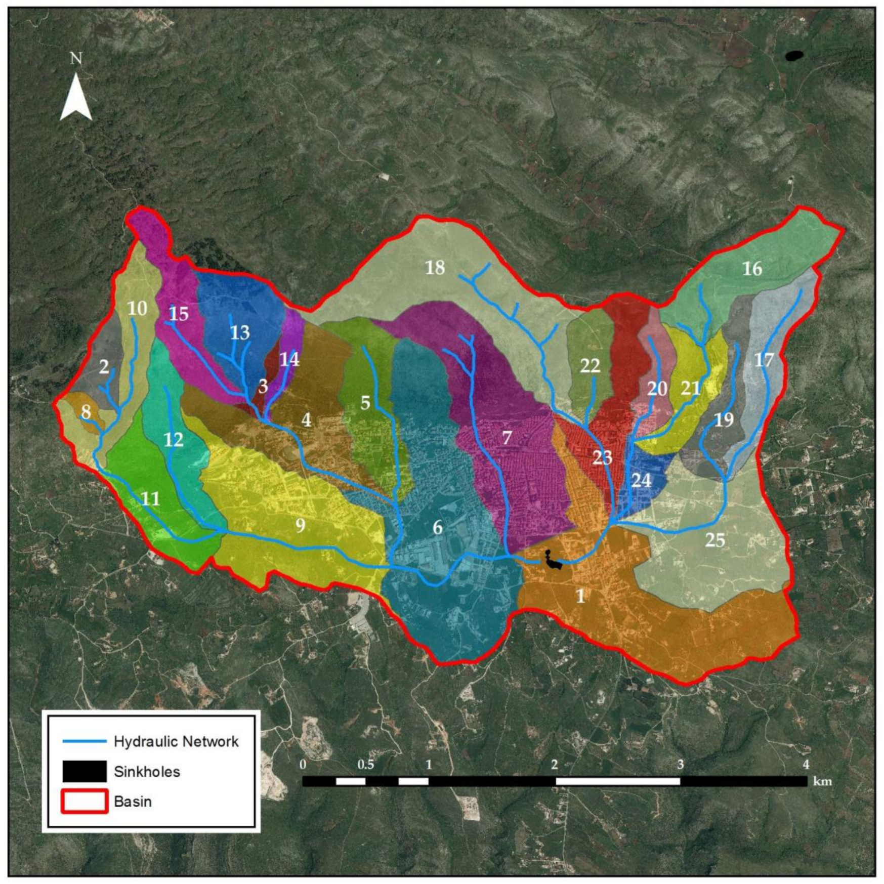
Using IDF curves, it was possible to provide the evaluation of the flood peak. First, the spatial scale of analysis for the delineation of the flow rate was defined. The whole basin was divided into 25 sub-basins, as shown in Figure 3, following the topography of the area and the hydrographic stream network.
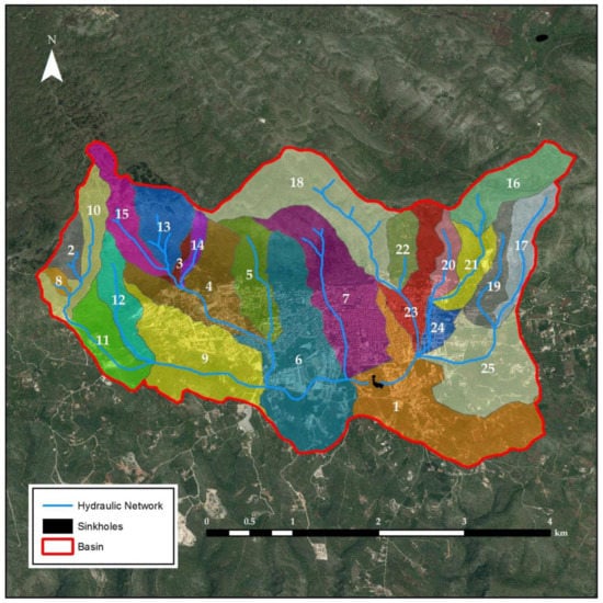
Figure 3.
Sub-basins map.
Sub-basins are numbered from 1 to 25. In order to estimate floods for several return periods, two types of data are needed: digital elevation data (DEM) and land use data. For hydraulic modeling, a Digital Elevation Model (DEM) with an 8-m cell size was used over the Apulia region.
The land use parameter was taken into account using the runoff curve number method. The method, proposed by the USDA Soil Conservation Service Agency (SCS-CN), is largely used in hydrology as a simple watershed model [37,38].
The wide use of this method is due to its applicability in different environments, its simplicity, and its dependence from soil types, land use, and antecedent moisture conditions [39].
The CN parameter takes into account three basic factors: the lithology of land, the characteristics of land use, and agricultural practices. The CN variation range is from 0 to 100; therefore, for each sub-basin floods were estimated using a semi-distributed model.
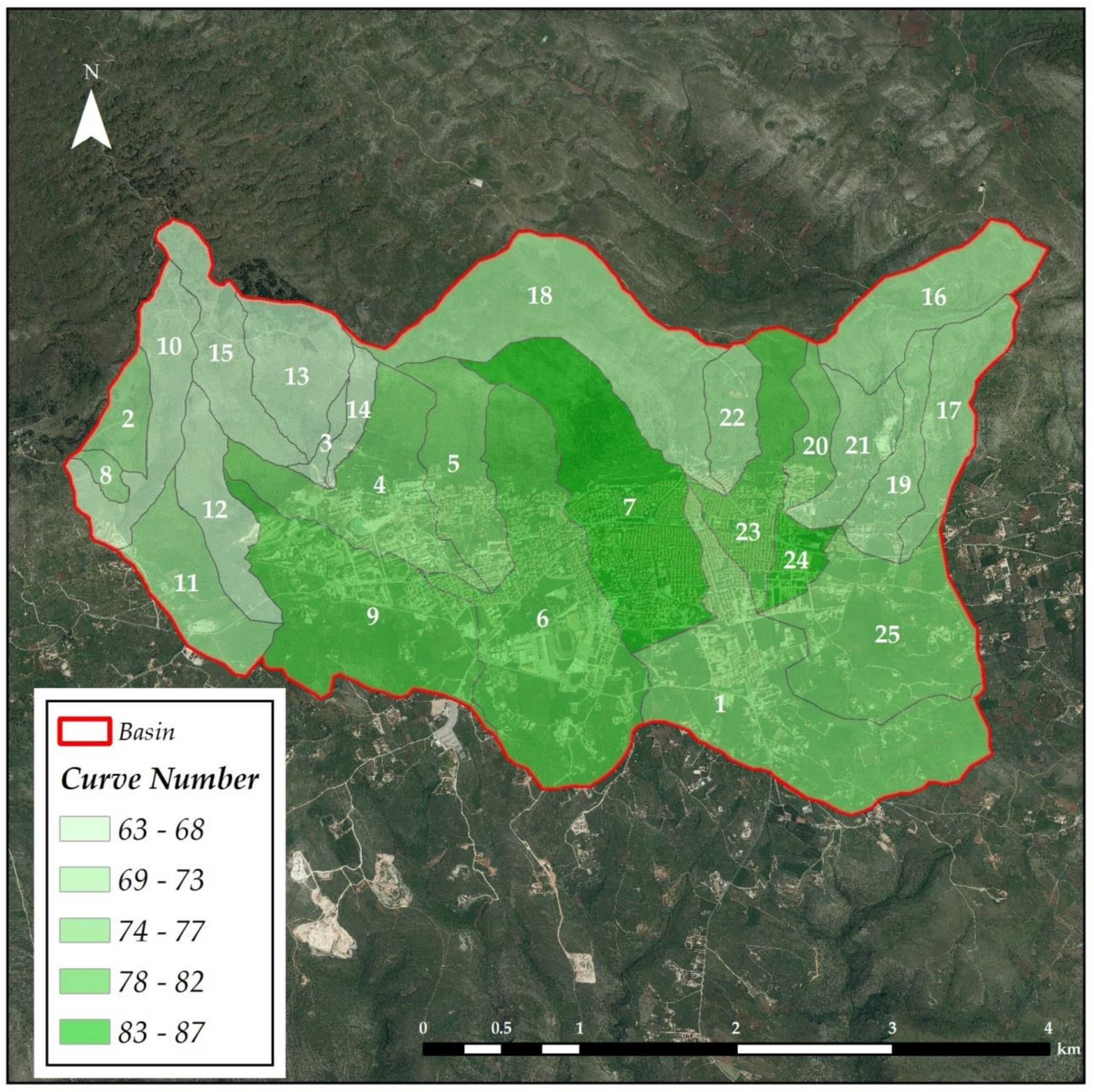
Finally, for all sub-basins, average height, slope, surface, length of main stream, and CNII values were calculated [40]. A map of the CN value for each sub-basin is given in Figure 4.

Figure 4.
Curve number nap.
In Table 2, the flow rates are reported in m3/s.

Table 2.
Flow rates for several return periods.
In order to evaluate the flow depth and the velocity of floods for each return period, a two-dimensional numerical model called FLO-2D [41] was utilized. Three numerical simulations were performed using an empirical approach, evaluating the peak flow rate and the triangular hydrograph for each sub-basin with a return period respectively equal to 30, 200, and 500 years.
The choice of the return periods was made according to the PAI Puglia (i.e., the hydrogeological setting plan) [28]. This approach has provided the “hydraulic hazard” in the study area.
Numerical simulations were carried out in a system of square grid elements, with a width equal to 8 m. In particular, the DEM adopted to simulate flow on a floodplain topography was provided by the Regional Authorities of Apulia. The roughness parameter used for modeling is a Manning uniform coefficient equal to 0.04 s/m1/3, which is the mean value for all of the basins.
The simulation of the flooding was obtained through the numerical integration of the conservation equation of fluid volume and the Motion equation (full dynamic wave momentum equation) [41].
The model performed with a simulation time of 8 h. Instead, the computational times are: 2.90 h for 30 years (scenario1); 3.14 h for 200 years (scenario 2); 3.67 h for 500 years (scenario 3).
It should be noted that, to analyze the effects of the hydraulic simulations, the results are filtered, leaving out areas that experienced only marginal flooding.
In fact, after running the simulation, some areas included in flooding zones presented values of flow depth and velocity that were negligible to the actual consequences; these areas were defined as “marginal” with respect to the risk connected to the flooding events.
In order to define the safety area limits, the equation line passing by the points (0.2, 0) and (0.52, 0) on the plane (h, v) was chosen, with flow depth expressed in meters and velocity in meters per second, in accordance with the Basin Regional Authority. The equation used to define the filtered areas is the following:
h* represents the maximum acceptable “flow depth” value to neglect the practical effects. In this way, each cell presenting a value of “flow depth” h lower than the corresponding limit value of h*, calculated as a function of the flow velocity, was considered to be in a hydraulic safety condition.
3.3. Risk Assessment
A quantitative assessment of the exposure, in terms of monetary values, of the elements at risk and consequently of the associated risk, in terms of economic losses, was carried out. This assessment aimed to quantify economically tangible and direct damages due to potential flood events, which are physical damages to building, infrastructures, and agriculture.
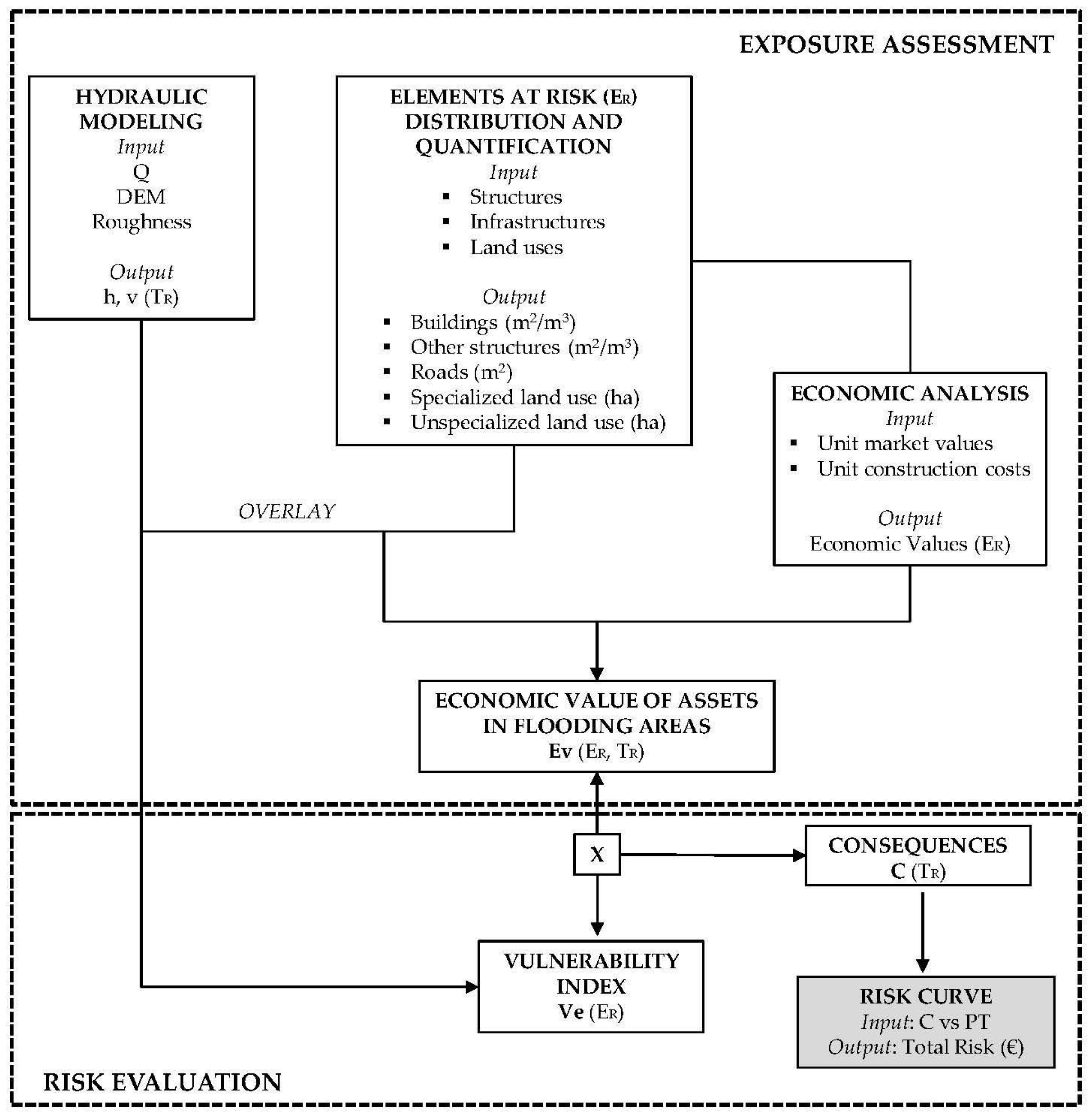
In order to conduct this quantitative assessment, five categories of elements at risk were considered for the analysis: buildings, other structures, infrastructures, and specialized and unspecialized land use (Figure 5). A total of 26 sub-categories of exposed assets were selected from the abovementioned: hotel, sport areas, paved parking, electric cabin, gas cabin, agricultural sheds, cemetery chapel, church, landfill, building, hospital, silos, energy areas, urban roads, tree planted areas, orchards, unqualified garden, nude, vegetable garden, arable crops, olive groves, vineyards, conifer forests, deciduous forests, shrub pasture, and mixed forests.

Figure 5.
Proposed methodological approach for exposure and risk estimation.
As a result of various motives, population was not considered among the elements at risk. First at all, the literature defines population as part of the intangible losses [11]. Moreover, there are objective difficulties both in assessing the temporal and spatial distribution of people in an urban center and the ethical dilemma in quantifying the economic value associated with injuries or deaths. Population is a mobile asset [42] and, for this reason, the evaluation of the exposure of persons would require the calculation of the conditional probability of persons being present in buildings or on the roads at the time of occurrence of a natural hazard [43].
The procedure used to quantitatively evaluate the exposure of elements at risk was derived from Pellicani et al., 2014 [14] and consisted in the overlay of the elements with each hydraulic hazard map, followed by the evaluation of the amount of assets in each flooding area and the quantification of the economic values affected by the various flood hazard scenarios (Figure 5).
Each type of element at risk was quantified in terms of areal extent (square meters and hectares). The information on the spatial distribution of assets was combined individually with the three hydraulic hazard maps, in order to obtain the number of elements potentially affected by flooding with a return period of 30, 200, and 500 years.
The spatial distribution of the three macro-categories of elements at risk was derived from the Regional Technical Map of Apulia at a 1:5000 scale, for structures and infrastructures, and from the Land Use Map of Apulia at a 1:5000 scale, for land use category, both available at the geo-portal of the Apulia region [44].
Therefore, in order to evaluate the economic exposure associated with the different hydraulic hazard levels, the unit market values or unit construction costs were assumed for each asset category. Starting from buildings, the unit market value (Euros per square meter) relative to 2017 was obtained from the Observatory of Real Estate Market (OMI) instituted by the National Territorial Agency. OMI is a cadastral database and provides maximum and minimum values for different kinds of buildings, such as residential, commercial, agricultural, etc., and for different zones of inhabited area, such as city centers, suburbs, etc. A mean among the values related to residential and commercial buildings, considering the overall percentage of the second ones with respect to the first ones in the study area, was derived. As far as hotels, churches, and hospitals were concerned, the unit construction costs (Euros per cubic meter) were deduced from the DEI National Price List for 2017.
For sport areas, paved parking, electric cabins, gas cabins, agricultural sheds, cemetery chapels, landfills, silos, and energy areas, the unit construction costs (Euros per square meter or cubic meter) were calculated from values defined in 1988–1989 by the National Territorial Agency. These values were updated by calculating the inflation rate using data from ISTAT (National Institute of Statistics). Also, the unit agricultural values (Euros per hectare) were obtained from the National Territorial Agency. The most recent data for the study area (included in the Foggia Province) are related to 2012. Finally, for roads, the unit construction costs obtained from the Regional Price List of Apulia for 2017 were used.
After defining the monetary value of the 26 elements at risk categories, a quantitative analysis of their exposure was carried out. Therefore, the exposed values associated with each flooding scenario were quantified by multiplying the amount of the individual exposed assets (square meters, cubic meters, and hectares) with their unit economic value.
The quantitative evaluation of risk associated with the three flood hazard scenarios, in terms of economic expected losses, was carried out starting from the exposure estimation, according to Figure 5.
For each category of elements at flood risk, the potential damages were obtained by considering their vulnerability to flood damages, expressed by flood damage functions. Velocity and flood depth values, resulting from the hydraulic modeling and varying for each flood hazard scenario, permitted the calculation of a vulnerability (Ve) value, ranging from 0 to 1 (Table 3). Therefore, Ve defines the percentage of damages as a function of the physical characteristics of floodwaters. As a matter of fact, each sub-category of the five abovementioned categories was associated with a different vulnerability flood damage function. The flood damage functions of buildings, other structures, as well as specialized and unspecialized land use were referred to Barbano et al., 2012 [15], whereas that of infrastructures was referred to Huizinga et al., 2017 [16].

Table 3.
Flood damage functions.
The consequences were assessed by multiplying the exposed economic value of assets by the Ve values of each category of elements at risk.
For each flooding scenario, the total consequences (or expected losses) were calculated by summing the values related to the five categories of elements at risk. The economic loss values resulting from each flooding scenario were plotted against the three-temporal probability of hazard scenarios in order to obtain the risk curve. Finally, the area under the curve was determined, representing the total flooding risk in monetary terms.
This methodology was applied to the study area and to each sub-basin represented in Figure 3 in order to classify the areas more impacted by flood damages.
4. Results and Discussion
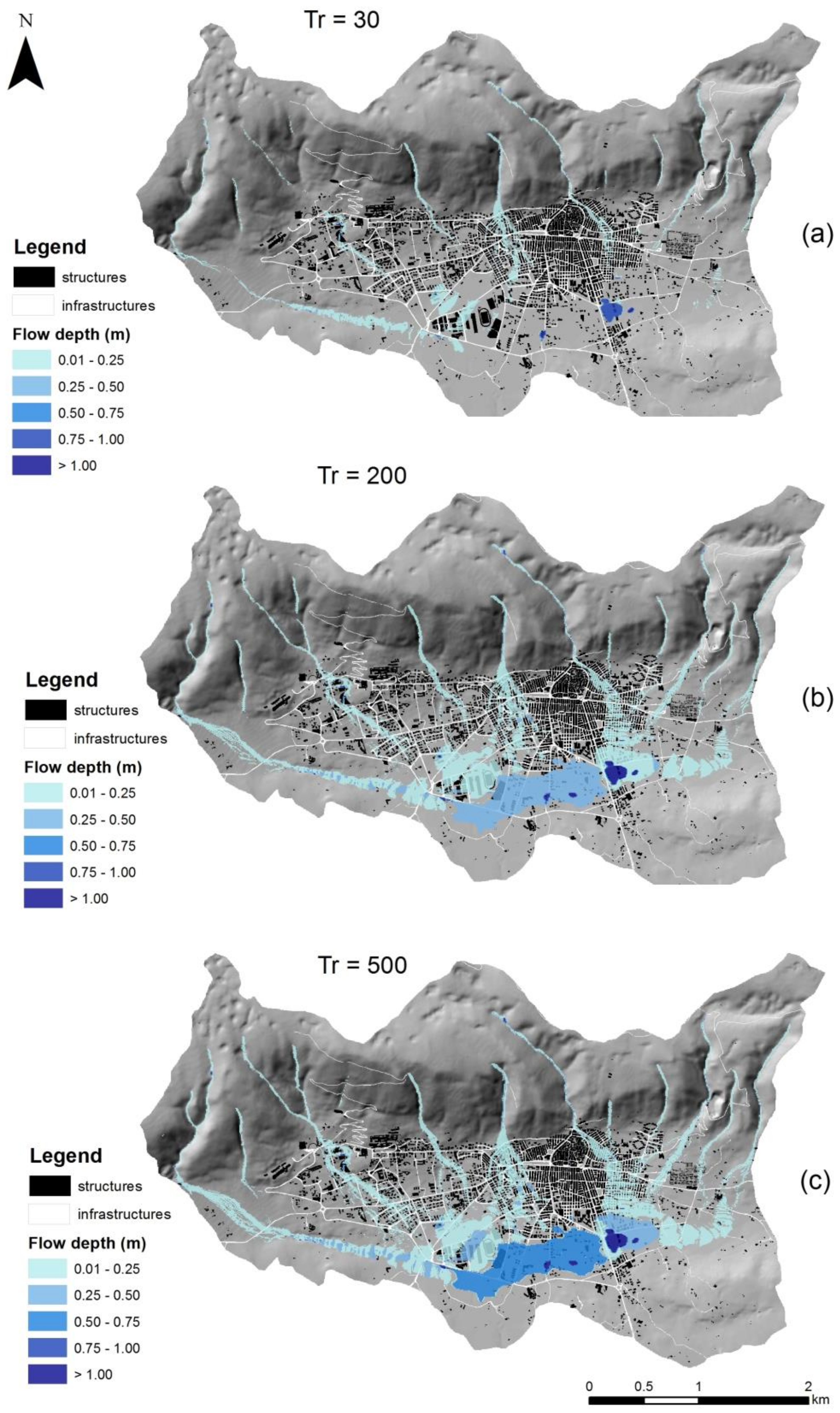
After the definition of all parameters using the FLO-2d model, the hydraulic model was performed. The results of the two-dimensional numerical models were examined for all return periods investigated. The flooding areas for the three scenarios are shown in Figure 6. The results show an evolution of the extension of the flood area, as well of the flow depth and velocity, proportional to the increase of the return period.
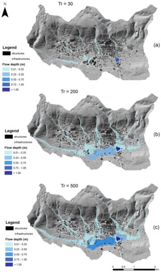
Figure 6.
Flooding areas for the three hazard scenarios with return period of 30 (a), 200 (b) and 500 (c) years.
A comparative analysis between the different scenarios in the domain was also carried out. In particular, the areas most affected in terms of flow depth are those most depressed, placed in the new expansion zone of the town at the boundary of the historical settlement. Meanwhile, in terms of velocity, the highest values were recorded along the flow directions with the highest slope, to then pour into the preferential accumulation zones described above.
The hydraulic model calibration was conducted on the basis of flooding reports. The results in terms of “flooding areas” demonstrate the need for an upgrade of the real hazard map in San Giovanni Rotondo. In fact, this study finally provided a valid tool for Civil Protection in terms of the “flooding forecast”, as well as a tool for the Basin Regional Authority in terms of “flood hazard management”.
In particular, the numerical analysis, conducted at the basin scale, highlighted some critical areas in relation to the flow capacity in safety conditions.
It seems evident that an accurate estimation of flooding hazard, already highlighted in the scenario characterized by the minor return period (TR), would significantly improve the real-time management of flood risk in the study area.
The analysis of the exposure of assets affected by the three flooding scenarios in the whole study area allowed for the categorization of the different typologies of elements in order of amount and economic exposed values, as shown in Table 4.

Table 4.
Definition, for each element at risk category and flooding scenario, of amount, economic value of exposed assets, and overall consequences.
It is important to note that the amount in square meters of the different kinds of structures, especially residential buildings, refers to the areal extent in plan. The overall amount of buildings, used to calculate the economic values of structures potentially damaged by flooding, was computed considering the height of buildings or the number of floors. This data was obtained by extracting the absolute altitude from the elevation points of the Regional Technical Map related to building eaves and by subtracting from this the terrain elevation.
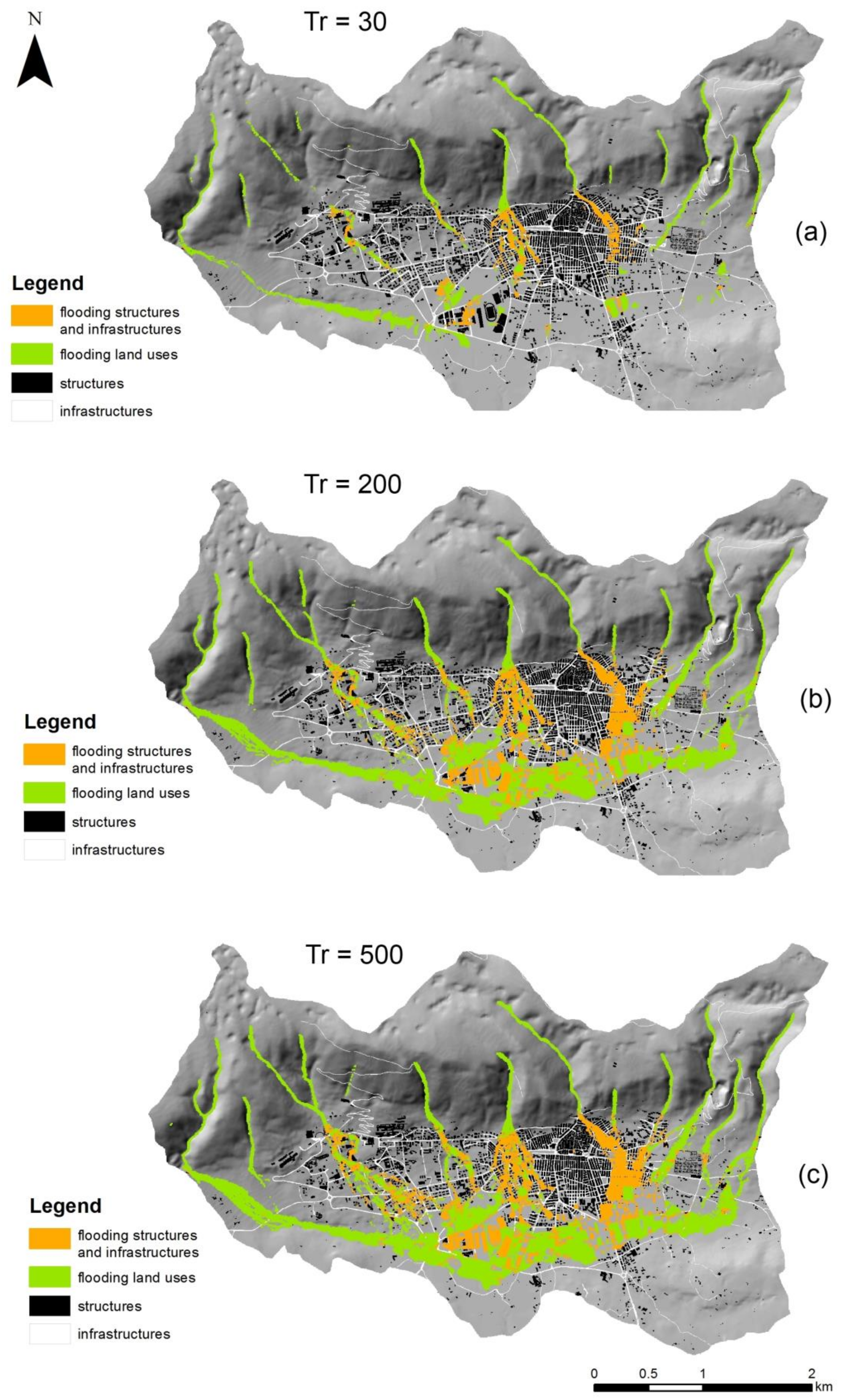
The spatial distribution of the elements at risk included in the three flooding areas and grouped into land uses, structures, and infrastructures is shown in Figure 7.
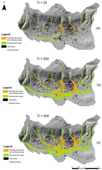
Figure 7.
Elements at risk in flooding areas for the three hazard scenarios with return period of 30 (a), 200 (b) and 500 (c) years.
In the area of study, the Regional Authority has already considered structural hydraulic defense works to mitigate flood risk for a return period of 200 years, at a cost of about €7,000,000.00 [45]. It is thus appreciable to highlight that this economic amount would be lower than the economic estimation of tangible and direct losses related to a 30-year return period.
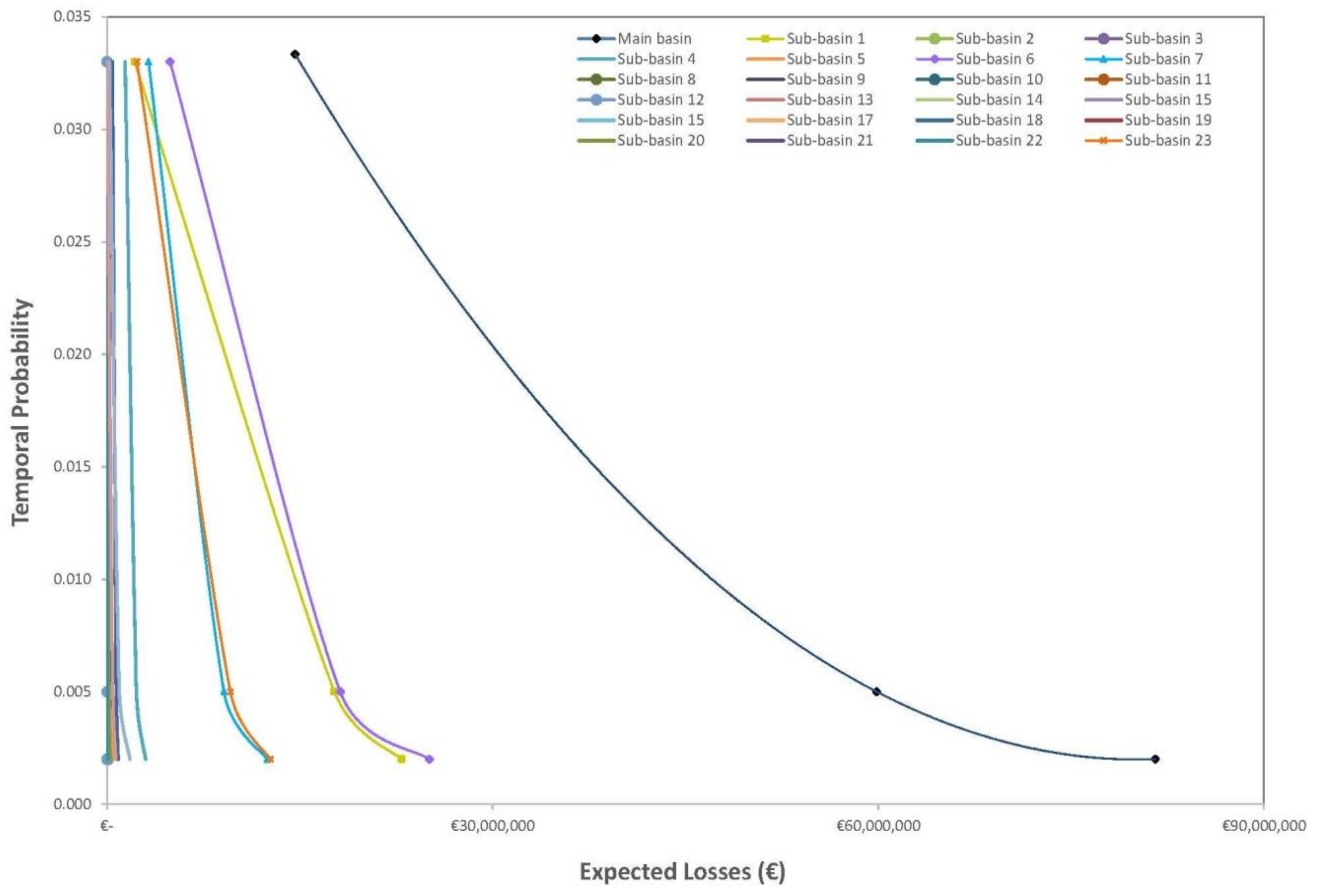
The risk curve, obtained by plotting the values of total economic losses and temporal probabilities summarized in Table 4, is shown in Figure 8. The total flooding risk in monetary terms was estimated, by calculating the area under the curve, to be equal to €806,268.
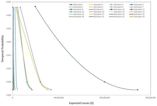
Figure 8.
Risk curves for the main basin and sub-basins.
In order to obtain a better definition and knowledge of the distribution of the risk level in the study area, the quantification of the expected losses in the 25 sub-basins was carried out. In Figure 8, the risk curves for each of the 25 sub-basins are plotted. The total flooding risk values in monetary terms for each sub-basin are summarized in Table 5 and mapped in Figure 9. It can be observed that sub-basins 1, 6, 7, and 23 provide greater contributions to the total risk of the main basin. In particular, sub-basin 1 and the lower portions of sub-basins 6 and 7 correspond to areas of recent urban expansion.

Table 5.
Total risk for sub-basins.
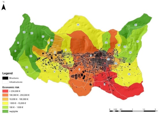
Figure 9.
Ranking map of the 25 sub-basins according to economic flooding risk.
This study may represent a decision support system to delineate the actions that in the future will have to be prepared in order to define safety interventions for these areas recently affected by flooding. In particular, using a basin scale approach, it is also possible to provide a “priority order” for the coordination of “structural interventions for the reduction of flooding risk”. The approach proposed (at the basin scale) in this manuscript is in line with the European Parliament Directive 2007/60/EC of 23 October 2007 on the assessment and management of flood risks. In fact, as said in the directive “the management of flood risks should be determined by the Member States themselves and should be based on local and regional circumstances”.
In the evaluation of risk, the 2007/60/EC suggests to take into account “the particular characteristics of the areas they cover and provide for tailored solutions according to the needs and priorities of those areas, whilst ensuring relevant coordination within river basin districts and promoting the achievement of environmental objectives laid down in Community legislation”. In other words, the directive recommends this approach where it is necessary to consider population, economic assets, and ecologic value—not only the flooding hazard.
Finally, a method that quantifies the flooding risk through the estimation of the expected losses, in monetary terms, allows also the establishment of the changes of risk in the future with urban development and inflation.
5. Conclusions
Although studies on the assessment of risk associated with natural hazards (landslide, flooding, earthquakes, etc.) presented in the literature are increasing, the quantitative evaluation of risk, which expresses the expected monetary losses as the product of hazard (or probability of occurrence), amount or costs (of elements at risk), and vulnerability (the degree of damage of the elements at risk) is often hampered by severely limited data on the calamitous event, damages, costs, etc.
This study aims to define a methodology to assess the economic value of tangible and direct losses related to potential flood events. It undoubtedly has some constraints related to many drivers, such as hydrologic data and modeling, flood damage functions, and unit market values.
Despite these limitations, the method permits a comparison of tangible and direct losses both of cities at a wide scale and of sub-basin at an urban scale. This result can aid in addressing the financial resources of local governments towards areas more exposed to losses. In order to do this, we are aware that it will be fundamental to implement the methodology with the assessment of tangible and indirect losses at the local scale, due to the cascading effects of flooding on impacted systems.
Finally, this work may represent a decision support system to delineate the actions that in the future will have to be prepared to define safety interventions for these areas recently affected by flooding. A further upgrade of this work may be achieved, in order to also consider indirect and intangible losses at the basin scale.
Acknowledgments
The authors gratefully acknowledge the support received for English editing by CEng MICE Martino Abbattista.
Author Contributions
Roberta Pellicani and Alessandro Parisi conceived the work; Ciro Apollonio and Gabriele Iemmolo performed the hydrologic and hydraulic modeling; Roberta Pellicani and Alessandro Parisi performed risk analysis; Roberta Pellicani, Ciro Apollonio, Alessandro Parisi, and Gabriele Iemmolo analyzed the results. Ciro Apollonio drafted the manuscript. Roberta Pellicani and Ciro Apollonio revised the manuscript. All authors read and approved the final manuscript.
Conflicts of Interest
The authors declare no conflict of interest.
References
- United Nations International Strategy for Disaster Reduction Secretariat. Global Assessment Report on Disaster Risk Reduction; United Nations International Strategy for Disaster Reduction Secretariat: Geneva, Switzerland, 2009; pp. 1–207. ISBN 9789211320282. [Google Scholar]
- Carrera, L.; Standardi, G.; Bosello, F.; Mysiak, J. Assessing direct and indirect economic impacts of a flood event through the integration of spatial and computable general equilibrium modelling. Environ. Modell. Softw. 2015, 63, 109–122. [Google Scholar] [CrossRef]
- Apollonio, C.; Balacco, G.; Novelli, A.; Tarantino, E.; Piccinni, A.F. Land Use Change Impact on Flooding Areas: The Case Study of Cervaro Basin (Italy). Sustainability 2016, 8, 996. [Google Scholar] [CrossRef]
- Novelli, A.; Tarantino, E.; Caradonna, G.; Apollonio, C.; Balacco, G.; Piccinni, F. Improving the ANN Classification Accuracy of Landsat Data Through Spectral Indices and Linear Transformations (PCA and TCT) Aimed at LU/LC Monitoring of a River Basin. In Proceedings of the 16th International Conference on Computational Science and Its Applications, Beijing, China, 4–7 July 2016; Gervasi, O., Murgante, B., Misra, S., Rocha, A.M.A.C., Torre, C.M., Taniar, D., Apduhan, B.O., Stankova, E., Wang, S., Eds.; Springer: Beijing, China, 2016; pp. 420–432. [Google Scholar]
- European Environmental Agency. Economic Losses from Climate-Related Extremes. European Environmental Agency, 2017. Available online: https://www.eea.europa.eu/data-and-maps/indicators/direct-losses-from-weather-disasters-3/assessment/#economic-losses-from-climate-related-extremes (accessed on 29 March 2018).
- Glade, T.; Anderson, M.; Crozier, M.J. Landslide Hazard and Risk; John Wiley & Sons, Ltd.: Chichester, UK, 2005; pp. 1–824. ISBN 9780471486633. [Google Scholar]
- Pellicani, R.; Argentiero, I.; Parisi, A.; Fidelibus, M.D.; Spilotro, G. Resilience modification and dynamic risk assessment in hybrid systems. Study cases in underground settlements of Murgia edge (Apulia, Southern Italy). In International Conference on Computational Science and Its Applications; Gervasi, O., Murgante, M., Misra, S., Borruso, G., Torre, C.M., Rocha, A.M., Taniar, D., Apduhan, B.O., Stankova, E., Cuzzocrea, A., Eds.; Springer: Cham, Switzerland, 2017; Volume 10405, pp. 230–245. ISBN 978-3-319-62394-8. [Google Scholar]
- Armenakis, C.; Nirupama, N. Estimating spatial disaster risk in urban environments. Geomat. Nat. Hazards Risk 2013, 4, 289–298. [Google Scholar] [CrossRef]
- Merz, B.; Kreibich, H.; Schwarze, R.; Thieken, A. Assessment of economic flood damage. Nat. Hazards Earth Syst. Sci. 2010, 10, 1697–1724. [Google Scholar] [CrossRef]
- Dutta, D.; Herath, S.; Musiake, K. Direct Flood Damage Modeling Towards Urban Flood Risk Management; International Center for Urban Safety Engineering: Tokyo, Japan, 2001; pp. 127–143. [Google Scholar]
- Mekong River Commission Secretariat. Best Practise Guidelines for Flood Risk Assessment. The Flood Management and Mitigation Programme Component 2: Structural Measures & Flood Proofing in the Lower Mekong Basin. 2009. Available online: http://www.preventionweb.net/files/15958_mrcbestpractiseguidelinesforfloodri.pdf (accessed on 29 March 2018).
- Nones, M.; Pescaroli, G. Implications of cascading effects for the EU Floods Directive. Int. J. River Basin Manag. 2016, 14, 195–204. [Google Scholar] [CrossRef]
- Pescaroli, G.; Alexander, D. A definition of cascading disaster and cascading effects: Going beyond the ‘topping dominoes’ metaphor. Planet@Risk 2015, 3, 58–67. [Google Scholar]
- Pellicani, R.; Van Westen, C.J.; Spilotro, G. Assessing landslide exposure in areas with limited landslide information. Landslides 2014, 11, 463–480. [Google Scholar] [CrossRef]
- Barbano, A.; Braca, G.; Bussettini, M.; Dessì, B.; Inghilesi, R.; Lastoria, B.; Monacelli, G.; Morucci, S.; Piva, F.; Sinapi, L.; et al. Proposta metodologica per l’aggiornamento delle Mappe di Pericolosità e di Rischio—Attuazione della Direttiva 2007/60/CE Relativa alla Valutazione e alla Gestione dei Rischi da Alluvioni (Decreto Legislativo n.49/2010); ISPRA: Rome, Italy, 2012. Available online: http://www.isprambiente.gov.it/files/pubblicazioni/manuali-lineeguida/MLG_82_2012.pdf (accessed on 29 March 2018).
- Huizinga, J.; de Moel, H.; Szewczyk, W. Global flood depth-damage functions—Methodology and the database with guidelines. Joint Res. Center 2017. [Google Scholar] [CrossRef]
- Van Westen, C.J.; Luna, B.Q.; Franco, R.V. Development of training materials on the use of geo-information for multi-hazard risk assessment in a mountainous environment. In Proceedings of the Mountain Risks International Conference, Firenze, Italy, 24–26 November 2010; Malet, J.-P., Glade, T., Casagli, N., Eds.; CERG: Strasbourg, France, 2010; pp. 469–475. [Google Scholar]
- Flood Directive 2007/60/EC of the European Parliament and of the Council of 23 October 2007 on the Assessment and Management of Flood Risks. Available online: http://eur-lex.europa.eu/legal-content/EN/TXT/?uri=CELEX:32007L0060 (accessed on 29 March 2018).
- Martinotti, M.E.; Pisano, L.; Marchesini, I.; Rossi, M.; Peruccacci, S.; Brunetti, M.T.; Melillo, M.; Amoruso, G.; Loiacono, P.; Vennari, C.; et al. Landslides, floods and sinkholes in a karst environment: The 1–6 September 2014 Gargano event, southern Italy. Nat. Hazards Earth Syst. Sci. 2017, 17, 467–480. [Google Scholar] [CrossRef]
- Billi, A.; Salvini, F. Sistemi di fratture associati a faglie in rocce carbonatiche: Nuovi dati sull’evoluzione tettonica del Promontorio del Gargano. Boll. Soc. Geol. Ital. 2000, 119, 237–250. [Google Scholar]
- Patacca, E.; Scandone, P. Geology of the Southern Apennines. Ital. J. Geosci. 2007, 7, 75–119. [Google Scholar]
- Sezione di Protezione Civile—Regione Puglia, Annali Idrologici. Available online: http://www.protezionecivile.puglia.it (accessed on 29 March 2018).
- Pellicani, R.; Spilotro, G. Evaluating the quality of landslide inventory maps: Comparison between archive and surveyed inventories for Daunia region (Apulia, Southern Italy). Bull. Eng. Geol. Environ. 2015, 74, 357–367. [Google Scholar] [CrossRef]
- Spilotro, G.; Gallicchio, S.; Pellicani, R.; Diprizio, G. A basic geothematic map for land planning and modeling (Daunian Subapennine—Apulia Region, Italy). In Proceedings of the Computational Science and Its Applications—16th International Conference, Beijing, China, 4–7 July 2016; Springer International Publishing: Cham, Switzerland, 2016; Volume 9788, pp. 107–119. [Google Scholar]
- Rossi, F.; Fiorentino, M.; Versace, P. Two-Component Extreme Value Distribution for Flood Frequency Analysis. Water Resour. Res. 1984, 20, 847–856. [Google Scholar] [CrossRef]
- Fiorentino, V.; Gabriele, S.; Rossi, F.; Versace, P. Hierarchical approach for regional flood frequency analysis. In Regional Flood Frequency Analysis; Singh, V.P., Ed.; D. Reidel: Norwell, MA, USA, 1987; pp. 35–49. [Google Scholar]
- Copertino, V.A.; Fiorentino, M. Valutazione Delle Piene in Puglia; Tipolitografia La Modernissima: Lamezia Terme, Italy, 1994. [Google Scholar]
- Autorità di Bacino della Puglia, Piano Stralcio di Assetto Idrogeologico (PAI). Available online: http://www.adb.puglia.it (accessed on 29 March 2018).
- U.S. Weather Bureau. Rainfall intensity-frequency regime—Part 1: The Ohio Valley. In Technical Paper No. 29 (TP-29); U.S. Weather Bureau: Washington, DC, USA, 1957. [Google Scholar]
- U.S. Weather Bureau. Rainfall intensity-frequency regime—Part 2: The Southeastern United States. In Technical Paper No. 29 (TP-29); U.S. Weather Bureau: Washington, DC, USA, 1958. [Google Scholar]
- U.S. Weather Bureau. Rainfall intensity-frequency regime—Part 3: The Middle Atlantic Region. In Technical Paper No. 29 (TP-29); U.S. Weather Bureau: Washington, DC, USA, 1958. [Google Scholar]
- U.S. Weather Bureau. Rainfall intensity-frequency regime—Part 4: The Northeastern United States. In Technical Paper No. 29 (TP-29); U.S. Weather Bureau: Washington, DC, USA, 1959. [Google Scholar]
- U.S. Weather Bureau. Rainfall intensity-frequency regime—Part 5: The Great Lakes Region. In Technical Paper No. 29 (TP-29); U.S. Weather Bureau: Washington, DC, USA, 1960. [Google Scholar]
- U.S. Weather Bureau. Two- to ten-day precipitation for return periods of 2 to 100 years in the contiguous United States. In Technical Paper No 49 (TP-49); U.S. Weather Bureau: Washington, DC, USA, 1964. [Google Scholar]
- Penta, A. Distribuzione di probabilità del massimo annuale dell’altezza di pioggia giornaliera su un bacino. In Proceedings of the Atti XIV Convegno di Idraulica e Costruzioni Idrauliche, Napoli, Italy, 10–12 October 1974. [Google Scholar]
- Eagleson, P.S. Dynamics of flood frequency. Water Resour. Res. 1972, 8, 878–898. [Google Scholar] [CrossRef]
- NRCS. National Engineering Handbook: Part 630—Hydrology Natural Resources Conservation Service; NRCS: Washington, DC, USA, 2004.
- Deshmukh, D.S.; Chaube, U.C.; Hailu, A.E.; Gudeta, D.A.; Kassa, M.T. Estimation and comparison of curve numbers based on dynamic land use land cover change, observed rainfall-runoff data and land slope. J. Hydrol. 2013, 492, 89–101. [Google Scholar] [CrossRef]
- Kowalik, T.; Walega, A. Estimation of CN parameter for small agricultural watersheds using asymptotic functions. Water 2015, 7, 939–955. [Google Scholar] [CrossRef]
- Mishra, S.K.; Singh, V. Soil Conservation Service Curve Number (SCS-CN) Methodology; Kluwer Academic Publishers: Dordrecht, The Netherlands, 2013; p. 42. [Google Scholar]
- O’Brien, J. FLO-2D Users Manual; FLO-2D Inc.: Nutrioso, AR, USA, 2001. [Google Scholar]
- Lee, E.M.; Jones, D.K.C. Landslide Risk Assessment; Thomas Telford Publishing: London, UK, 2014; p. 454. ISBN 0-7277-3171-8. [Google Scholar]
- Van Westen, C.J.; Van Asch, T.W.J.; Soeters, R. Landslide hazard and risk zonation—Why is it still so difficult? Bull. Eng. Geol. Environ. 2006, 65, 167–184. [Google Scholar] [CrossRef]
- SIT Puglia, Cartografia Tematica. Available online: http://www.sit.puglia.it/portal/portale_cartografie_tecniche_tematiche/home (accessed on 29 March 2018).
- Distretto Idrografico dell’Appennino Meridionale. Autorità di Bacino della Puglia. Available online: http://www.adb.puglia.it/public/page.php?96 (accessed on 29 March 2018).
© 2018 by the authors. Licensee MDPI, Basel, Switzerland. This article is an open access article distributed under the terms and conditions of the Creative Commons Attribution (CC BY) license (http://creativecommons.org/licenses/by/4.0/).

