Hydrodynamic and Debris-Damming Failure of Bridge Decks and Piers in Steady Flow

Abstract
1. Introduction
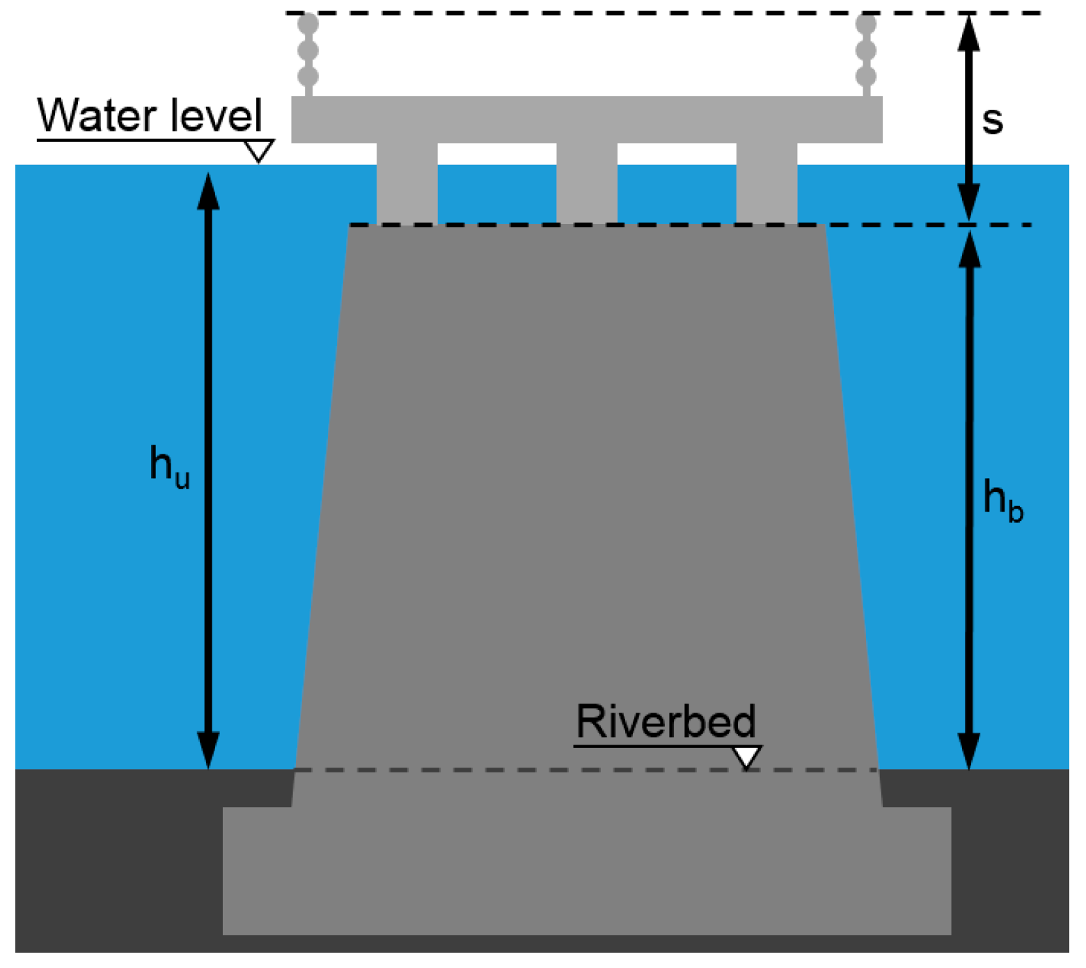
2. Materials and Methods
3. Results
3.1. Laboratory Experiments
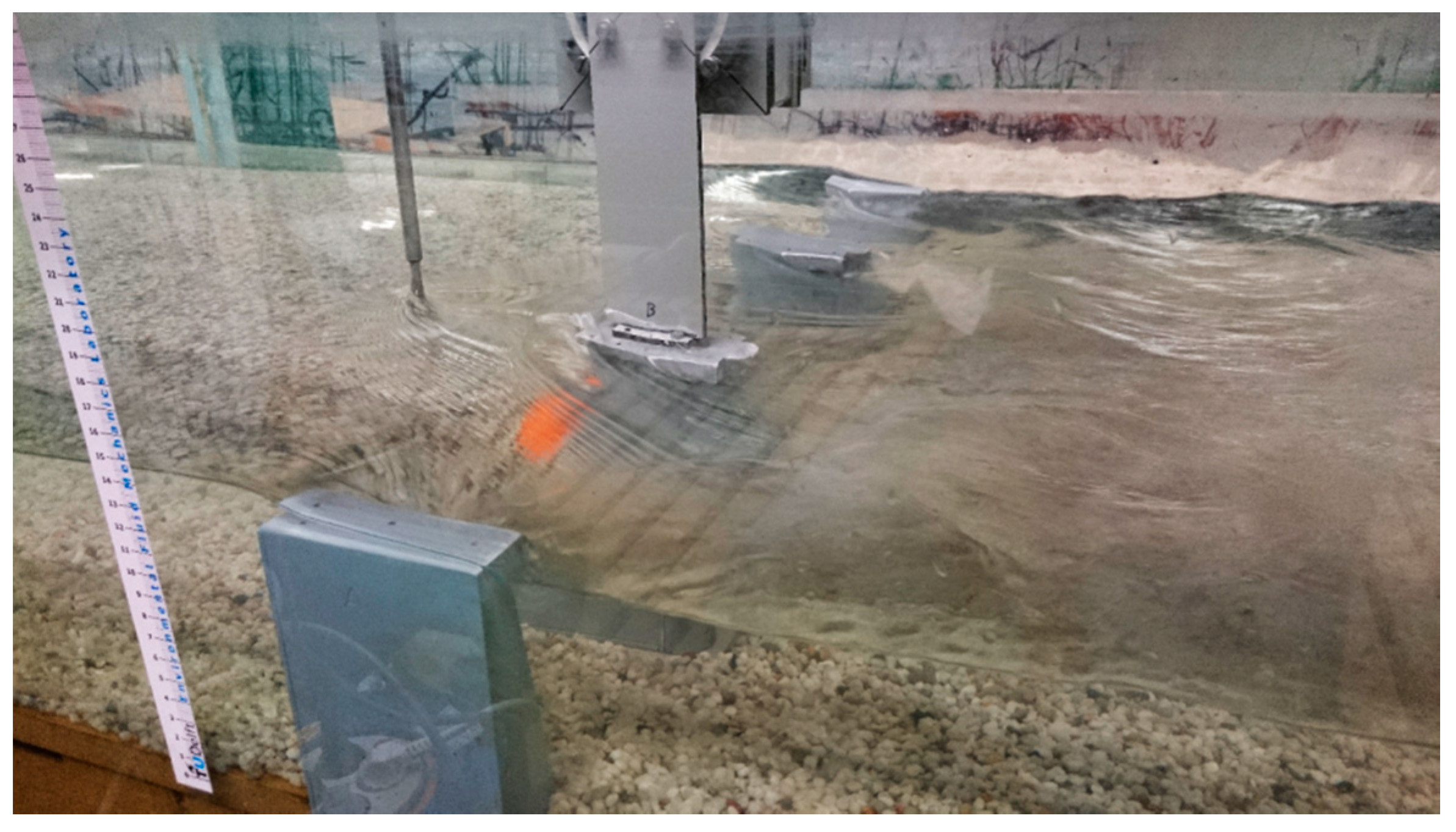
3.1.1. General
3.1.2. Rigidly Connected Deck-Pier System
3.1.3. Deck Failure Only (No Failure of Piers)
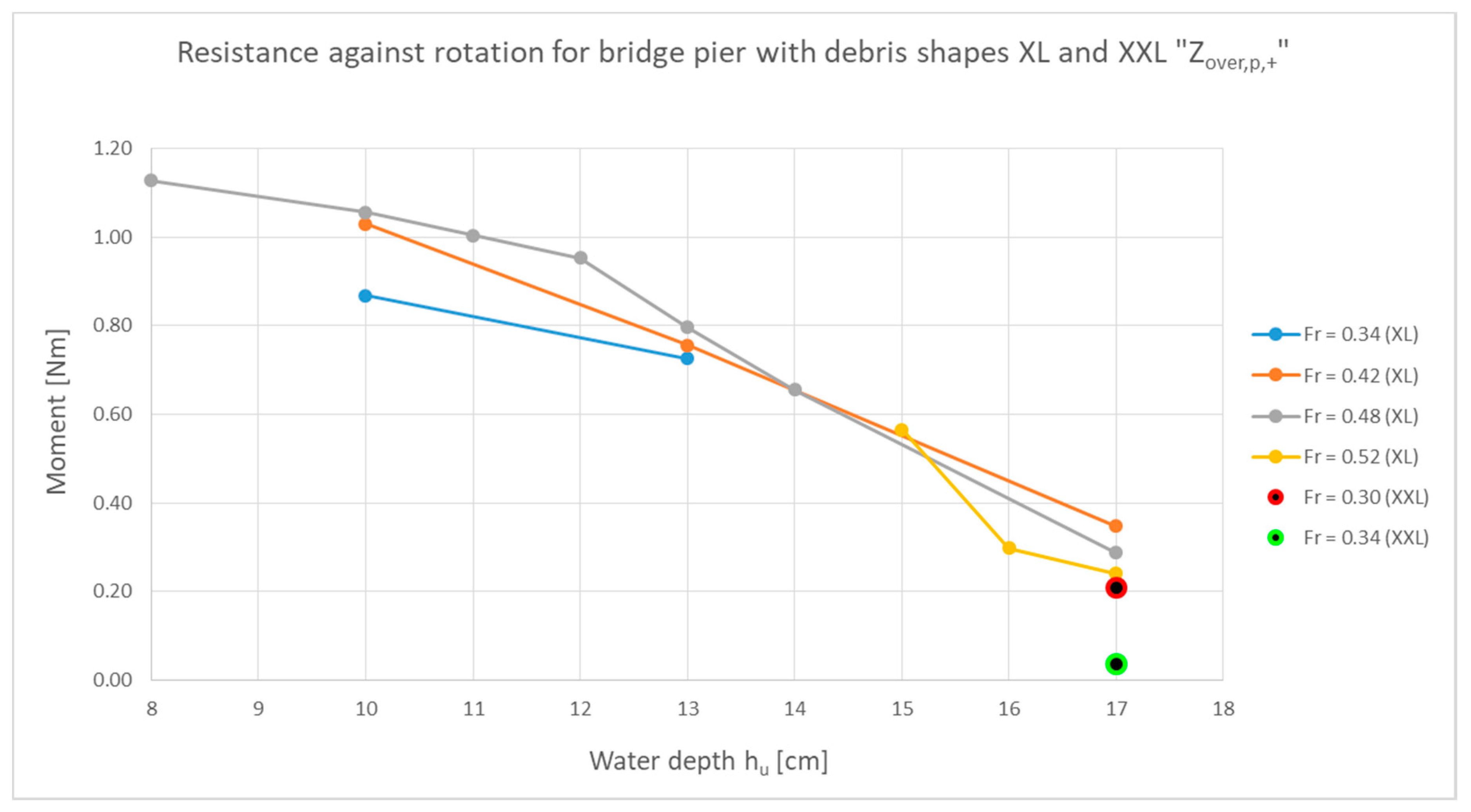
3.1.4. Pier Only (after Deck Failure)
3.2. Numerical Simulations
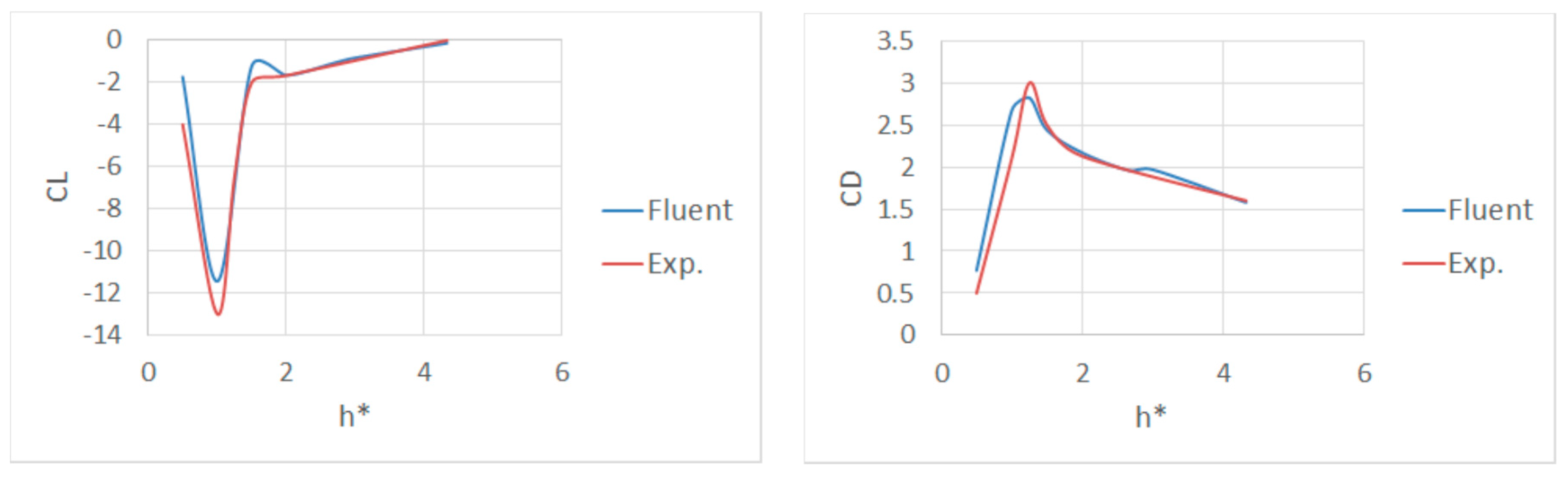
3.2.1. Validation
3.2.2. Effect of Proximity, Blockage, and Inundation Ratios on Bridge Deck Stability
Scenario 1: Fixed Proximity Ratio
Scenario 2: Fixed Blockage Ratio
Scenario 3: Fixed Inundation Ratio
3.2.3. Incipient Failure Analysis
3.2.4. Countermeasures
3.2.5. Comparison of Flow Patterns and Hydrodynamic Forces on a Box Deck and a Three Girder Deck
4. Discussion
5. Conclusions
Author Contributions
Funding
Acknowledgments
Conflicts of Interest
References
- Flint, M.M.; Fringer, O.; Billington, S.L.; Freyberg, D.; Diffenbaugh, N.S. Historical Analysis of Hydraulic Bridge Collapses in the Continental United States. J. Infrastruct. Syst. 2017, 23, 04017005. [Google Scholar] [CrossRef]
- Bricker, J.D.; Nakayama, A. Contribution of trapped air, deck superelevation, and nearby structures to bridge deck failure during a tsunami. J. Hydraulic Eng. 2014, 140, 05014002. [Google Scholar] [CrossRef]
- Bricker, J.D.; Nakayama, A.; Takagi, H.; Mitsui, J.; Miki, T. Mechanisms of Damage to Coastal Structures due to the 2011 Great East Japan Tsunami. In Handbook of Coastal Disaster Mitigation for Engineers and Planners; Esteban, M., Takagi, H., Shibayama, T., Eds.; Elsevier: Amsterdam, The Netherlands, 2015; pp. 385–415. [Google Scholar]
- Richardson, E.V.; Davis, S.R. Evaluating Scour at Bridges; Hydraulic Engineering Circular No. 18; Federal Highway Administration: Washington, DC, USA, 2001.
- EU. EN 1991-1-6: Eurocode 1: Actions on Structures—Part 1–6: General Actions—Actions during Execution; Authority: The European Union per Regulation 305/2011, Directive 98/34/EC, Directive 2004/18/EC; EU: Brussels, Belgium, 2005. [Google Scholar]
- Kerenyi, K.; Sofu, T.; Guo, J. Hydrodynamic Forces on Inundated Bridge Decks; Report FHWA-HRT-09-028 of the Federal Highway Administration; Federal Highway Administration: Washington, DC, USA, 2009.
- Australian Bridge Design Code; Standards Australia International Ltd.: Sydney, Australia, 2004.
- Parola, A.C. Debris Forces on Highway Bridges. National Cooperative Highway Research Program; National Academy Press: Washington, DC, USA, 2000. [Google Scholar]
- Malavasi, S.; Guadagnini, A. Hydrodynamic Loading on River Bridges. J. Hydraulic Eng. 2003, 129, 854–861. [Google Scholar] [CrossRef]
- Jempson, M.A. Flood and Debris Loads on Bridges. Ph.D. Thesis, University of Queensland, Brisbane, Australia, 2000. [Google Scholar]
- Trelleborg Engineered Products: Elastomeric Bearing Pads & Strips. Available online: https://www.trelleborg.com/engineered-products/~/media/engineered (accessed on 18 May 2018).
- Oudenbroek, K. Experimental Research on Hydrodynamic Failure of River Bridges on Spread Footings. Master’s Thesis, Delft University of Technology, Delft, The Netherlands, 2018. [Google Scholar]
- Naderi, N. Numerical Simulation of Hydrodynamic Forces on Bridge Decks. Master’s Thesis, Delft University of Technology, Delft, The Netherlands, 2018. [Google Scholar]
- American Association of State Highway and Transportation Officials. AASHTO LRFD Bridge Design Specifications; American Association of State Highway and Transportation Officials: Washington, DC, USA, 2013. [Google Scholar]
- Ducrocq, T. Flow and drag force around a free surface piercing cylinder for environmental applications. Environ. Fluid Mech. 2017, 17, 629–645. [Google Scholar] [CrossRef]
- Yu, D.; Kareem, A. Two-dimensional simulation of flow around rectangular prisms. J. Wind Eng. Ind. Aerodyn. 1996, 62, 131–161. [Google Scholar] [CrossRef]
- Hamill, L. Bridge Hydraulics; E & FN Spon: London, UK, 1999; p. 344. [Google Scholar]
- West, G.S.; Apelt, C.J. Measurements of fluctuating pressures and forces on a circular cylinder in the Reynolds number range 104 to 2.5 × 10⁵. J. Fluids Struct. 1993, 7, 227–244. [Google Scholar] [CrossRef]


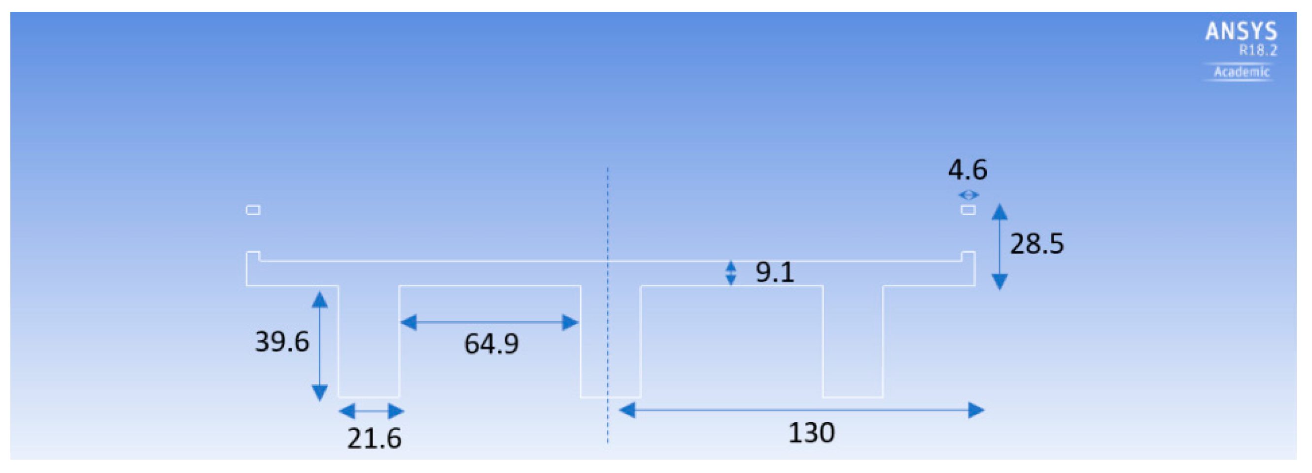
| Bridge Deck (Yellow) | Laboratory Model | Yabitsu Bridge (Actual) |
|---|---|---|
| Length (along road axis) | 254 mm | 9.4 m |
| Width (along river axis) | 142 mm | 5.3 m |
| Height | Girders: 19 mm Deck: 11 mm | Girders: 700 mm Deck: 410 mm |
| Base of the pier (red) | ||
| Length (along river axis) | Bottom:127 mm Top: 113 mm | Bottom: 4.7 m Top: 4.2 m |
| Width (along road axis) | Bottom: 41 mm Top: 49 mm | Bottom: 1.5 m Top: 1.8 m |
| Height | 129 mm | 4.8 m |
| Pier foundation (brown) | ||
| Length (along river axis) | 147 mm | 5.4 m |
| Width (along road axis) | 61 mm | 2.3 m |
| Height | 22 mm | 814 mm |
| Abutment (green) | ||
| Length (along river axis) | 96 mm | 3.6 m |
| Width (along road axis) | 76 mm | 2.8 m |
| Height | 151 mm | 5.6 m |
| Wet Weight (g) | Volume (cm3) | Frontal Area (cm2) | |
|---|---|---|---|
| Debris shape XXL | 382 | 545 | 100 |
| Debris shape XL | 292 | 417 | 83 |
| Hypothesis 1—deck—without debris | hu = 12.0 cm to 20.0 cm | Fr = 0.33 to 0.52 |
| Hypothesis 1—deck—with debris | hu = 13.0 cm to 19.0 cm | Fr = 0.10 to 0.52 |
| Hypothesis 1—pier—without debris | hu = 8.0 cm to 21.0 cm | Fr = 0.40 to 0.62 |
| Hypothesis 1—pier—with debris | hu = 8.0 cm to 17.0 cm | Fr = 0.34 to 0.52 |
| Hypothesis 2—combination—without debris | hu = 12.0 cm to 21.0 cm | Fr = 0.52 |
| Hypothesis 2—combination—with debris | hu = 16.0 cm to 21.0 cm | Fr = 0.52 |
| Flume Length (m) | Deck Length (m) | Deck Thickness, S (m) | hb (m) | hu (m) | Fr (−) |
|---|---|---|---|---|---|
| 5 | 0.18 | 0.06 | 0.14 | 0.1–0.4 | 0.1–0.15 |
| Time step size (s) | 0.005 |
| Iteration per time step | 20 |
| Multiphase model | Volume Of Fluid (VOF) |
| Pressure—velocity coupling scheme | Simple |
| Spatial discretization of momentum, turbulent kinetic energy, and specific dissipation rate | Second order upwind |
| Under relation factor for pressure | 0.3 |
| Under relaxation factors for remaining parameters | 0.7 |
| Mesh method/size | Multi-block technique/1 mm–1 cm |
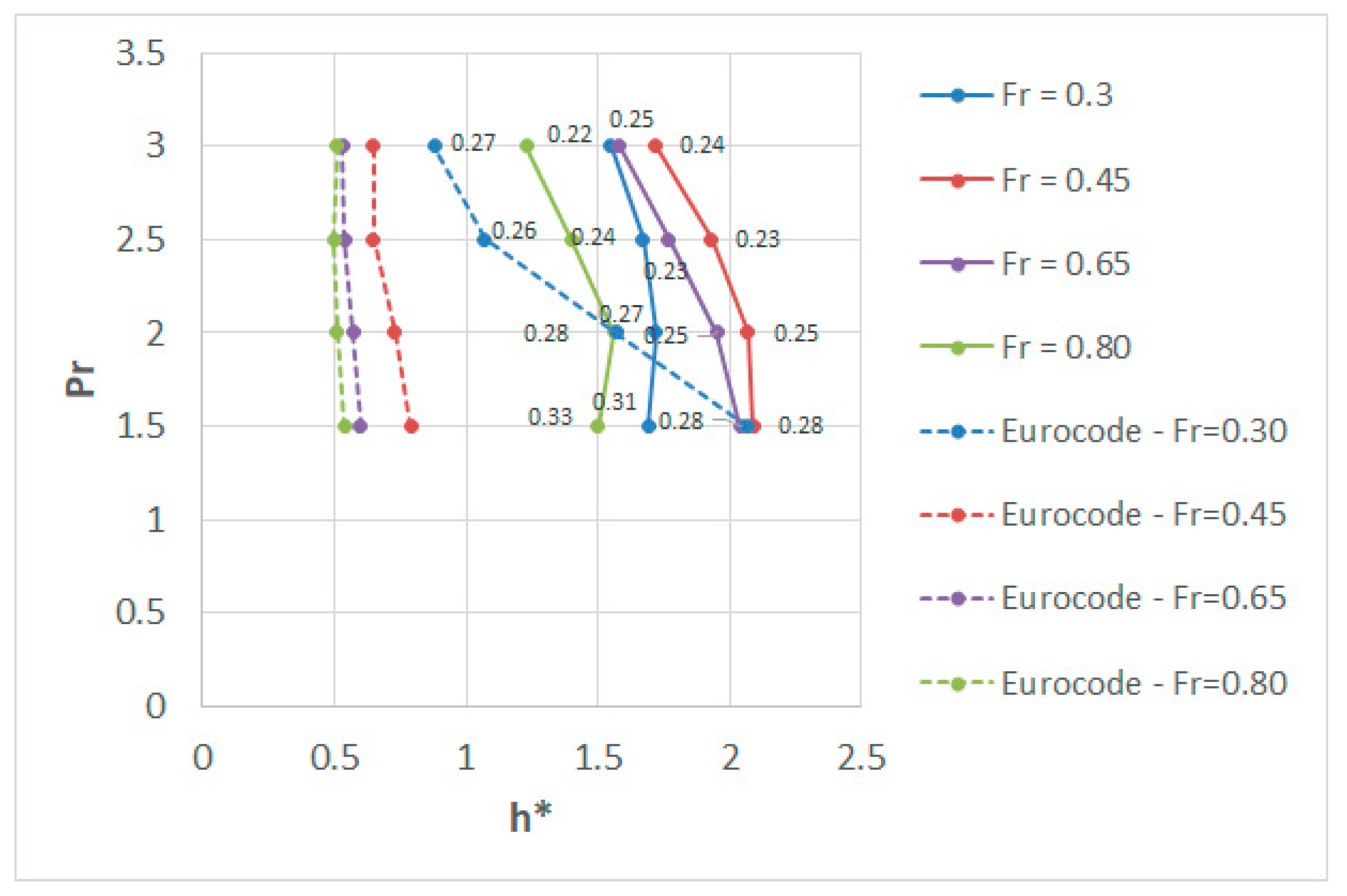
| Pr | h* | CD—AS5100 | CD—Numerical |
|---|---|---|---|
| 1.5 | 3 | 3.35 | 2.49 |
| 2 | 3 | 2.9 | 2.26 |
| 2.5 | 3 | 2.5 | 2.14 |
| 3 | 3 | 2.35 | 2.06 |
| 1.5 | 2 | 3.35 | 2.85 |
| 2 | 2 | 2.9 | 2.5 |
| 2.5 | 2 | 2.5 | 2.31 |
| 3 | 2 | 2.35 | 2.2 |
| 1.5 | 1 | 2.1 | 2.7 |
| 2 | 1 | 1.93 | 2.3 |
| 2.5 | 1 | 1.8 | 2.09 |
| 3 | 1 | 1.65 | 1.94 |
| Scenario 1 | Scenario 2 | Scenario 3 | Scenario 4 | Scenario 5 | Scenario 6 | |
|---|---|---|---|---|---|---|
| 1 | 0.5 | 0 | 1 | 0.5 | 0 | |
| 0.5 | 0.5 | 0.5 | 1 | 1 | 1 |
© 2018 by the authors. Licensee MDPI, Basel, Switzerland. This article is an open access article distributed under the terms and conditions of the Creative Commons Attribution (CC BY) license (http://creativecommons.org/licenses/by/4.0/).
Share and Cite
Oudenbroek, K.; Naderi, N.; Bricker, J.D.; Yang, Y.; Van der Veen, C.; Uijttewaal, W.; Moriguchi, S.; Jonkman, S.N. Hydrodynamic and Debris-Damming Failure of Bridge Decks and Piers in Steady Flow. Geosciences 2018, 8, 409. https://doi.org/10.3390/geosciences8110409
Oudenbroek K, Naderi N, Bricker JD, Yang Y, Van der Veen C, Uijttewaal W, Moriguchi S, Jonkman SN. Hydrodynamic and Debris-Damming Failure of Bridge Decks and Piers in Steady Flow. Geosciences. 2018; 8(11):409. https://doi.org/10.3390/geosciences8110409
Chicago/Turabian StyleOudenbroek, Kevin, Nader Naderi, Jeremy D. Bricker, Yuguang Yang, Cor Van der Veen, Wim Uijttewaal, Shuji Moriguchi, and Sebastiaan N. Jonkman. 2018. "Hydrodynamic and Debris-Damming Failure of Bridge Decks and Piers in Steady Flow" Geosciences 8, no. 11: 409. https://doi.org/10.3390/geosciences8110409
APA StyleOudenbroek, K., Naderi, N., Bricker, J. D., Yang, Y., Van der Veen, C., Uijttewaal, W., Moriguchi, S., & Jonkman, S. N. (2018). Hydrodynamic and Debris-Damming Failure of Bridge Decks and Piers in Steady Flow. Geosciences, 8(11), 409. https://doi.org/10.3390/geosciences8110409