Full-Flowfield Inversion of Debris-Flow Dynamics: A Global–Local Optimization Framework for Model Parameter Estimation from Final Accumulation Fields

Abstract

Calibration of debris-flow models is important for reproducible hazard mapping, transparent scenario analysis, and risk-informed territorial planning. Reliable calibration of debris-flow models is limited by parameter uncertainty, non-uniqueness, and the loss of spatial information when observations are reduced to scalar targets. This study presents a global–local full-flowfield inversion framework for estimating effective Voellmy friction parameters from complete final-thickness rasters, thereby replacing subjective trial-and-error adjustment with an explicit forward–inverse workflow and a spatially distributed objective function. A two-dimensional finite-volume shallow-flow solver is coupled with a genetic algorithm for bounded global exploration and projected finite-difference gradient descent for local refinement. The composite objective combines thickness, wet footprint, signed boundary distance, and total volume mismatches. The framework was evaluated through controlled parameter recovery, objective profiling, ten-seed repeatability tests, observation perturbations, conditional identifiability analysis, and a controlled Morino–Rendinara back-analysis retrieval test based on a published real-event parameterization and the real terrain. Uniform reference coefficients of 0.10, 0.25, and 0.45 were recovered with a mean absolute error of $1.90\times {10}^{-4}$ and exact wet footprint agreement. Across ten baseline inversions, the standard deviation of the estimate was $1.53\times {10}^{-4}$. Random removal of up to 50% of observation cells had negligible influence, whereas thickness noise and systematic scaling produced larger deviations; at 20% noise, mean IoU remained 0.9861. Prescribing $\xi$ between 250 and 1000 m s⁻² shifted the estimated $\mathsf{\mu }$ from 0.243038 to 0.254628 despite nearly identical final deposits, demonstrating conditional identifiability. In the two-zone experiment, the framework recovered ${\mathsf{\mu }}_{\mathrm{up}}=0.009991$ and ${\mathsf{\mu }}_{\mathrm{down}}=0.100184$, with a held-out RMSE of $4.49\times {10}^{-5}$ m and IoU equal to one. Full-flowfield inversion therefore provides accurate and reproducible event-specific parameter retrieval.

1. Introduction

Debris flows are rapid, gravity-driven mixtures of water, fine sediment, coarse particles, and entrained material. Debris flows occur in steep mountain environments worldwide and are among the most destructive rapid mass movements because high velocities, dense impact loads, and channelized routing can concentrate damage over very short time scales [1]. Their societal relevance is also evident from global event inventories: Dowling and Santi documented 213 fatal debris-flow events and 77,779 reported fatalities between 1950 and 2011 [2]. This makes debris-flow research particularly important where settlements, transport corridors, river crossings, and other exposed assets occupy narrow mountain valleys and alluvial fans. In Italy, the problem spans markedly different geomorphological settings. In the Italian Dolomites, integrated hazard assessments have shown how debris-flow activity can directly threaten roads and buildings and motivate structural mitigation and risk-zonation measures [3]; in northeastern Sicily, the 2009 rainstorm-triggered disaster involved hundreds of landslides, predominantly debris flows, and caused more than 30 fatalities, highlighting the consequences of rapid flow processes in densely urbanized terrain [4]. Their high velocities, large transported volumes, and impulsive forces can damage settlements, transport corridors, and critical infrastructure within very short time intervals. For this reason, reliable simulation and back-analysis are not only scientific objectives but also practical components of disaster-risk reduction, sustainable land-use planning, and the design of more resilient mountain communities. The classical synthesis by Iverson showed that grain friction, collisions, viscous stresses, and pore-fluid pressure can all contribute to debris-flow motion and that no single elementary constitutive law reproduces the full range of observed behaviour [5]. Later depth-averaged formulations incorporated increasingly detailed descriptions of mixture mechanics, pore-pressure effects, phase interaction, entrainment, and complex topography [6,7,8]. Although this development has improved physical representation, it has also increased the number of quantities that must be specified before a model can support event interpretation or hazard assessment. Calibration-based analyses show that simulated runout and deposition depend strongly on the adopted rheology and resistance parameters [9]. A widely used example is the Voellmy relation, which combines a Coulomb-like coefficient, $\mathsf{\mu }$, with a velocity-dependent turbulent coefficient, $\xi$ [10,11]. The coefficient $\mathsf{\mu }$ mainly controls frictional resistance, whereas $\xi$ regulates the quadratic resistance that becomes increasingly important at high velocity. In event back-analysis, however, these coefficients should be interpreted as effective model parameters rather than direct intrinsic properties of the material. They may incorporate unresolved effects associated with grain-size distribution, water content, pore pressure, surface roughness, entrainment, terrain resolution, and the assumptions introduced by depth averaging. Consequently, a parameter set that reproduces one event is not necessarily unique or transferable to another release condition or site.

Debris-flow back-analysis is generally performed by varying uncertain resistance parameters until selected simulated quantities agree with the available evidence. The Morino–Rendinara slope instability in central Italy was initially investigated as a cascading landslide system through an integrated geomorphological, remote-sensing, and numerical analysis, including the modelling of slope-scale prospective debris-flow propagation [12]. The site subsequently became a reference case for RAMMS-based debris-flow back-analysis and data-driven surrogate modelling [13,14,15]. In particular, the RAMMS back-analysis provided published information on the release representation, final accumulation, and spatially differentiated Voellmy coefficients [13]. More generally, calibration remains difficult because different combinations of parameters and uncertain inputs may generate similar outputs. This behaviour is related to equifinality in environmental modelling [16], parameter–discrepancy confounding in computer model calibration [17], and non-uniqueness in inverse theory [18]. A small residual therefore demonstrates agreement within the adopted model but does not, by itself, establish that the recovered parameters are physically unique. These experiences reinforce the need for dedicated debris-flow research and for calibration procedures that are explicit, reproducible, and transparent about parameter uncertainty rather than relying only on subjective trial-and-error adjustment.

Calibration-based forward analyses commonly vary rheological or resistance coefficients until runout, inundation extent, deposit geometry, flow depth, or other event descriptors are reproduced [9,13,19,20,21]. Several studies have also moved beyond purely manual trial-and-error adjustment. Iovine et al. used a genetic algorithm to calibrate a cellular-automata debris-flow model against the May 1998 Curti–Sarno event in southern Italy [22]; Brezzi et al. proposed a statistical data assimilation procedure to objectively select runout model parameters from pre- and post-event information [23]; and Calvello et al. formulated an inverse analysis in which the number and spatial distribution of deposit thickness observations explicitly affected calibration reliability [24]. More recent approaches additionally emphasize uncertainty quantification and computationally efficient parameter exploration, including Bayesian calibration and active learning strategies for landslide runout models [25].

The distinction between forward modelling and inversion is central to the present work. Forward modelling answers the question: given the terrain, release condition, material properties, boundary conditions, and resistance parameters, what flow evolution and final deposit are predicted? In mathematical terms, the forward operator maps a parameter vector $\mathit{\theta }$ to a simulated thickness field. Inversion addresses the reverse question: given an observed final accumulation field and a specified forward model, which parameter vector most closely reproduces that observation? Because this reverse mapping is not available in closed form, the inversion proceeds iteratively. An optimizer proposes a candidate parameter set, the forward solver generates the corresponding deposit, a mismatch function compares the simulated and observed fields, and the candidate parameters are updated until the mismatch is minimized. Most debris-flow calibrations condense the observation into a small number of scalar targets, such as maximum runout, inundated area, or total deposited volume. These quantities are useful but discard the spatial distribution of thickness within the deposit. In this study, the complete final-thickness raster is treated as the observation. The proposed full-flowfield inversion is conceptually analogous to full-waveform inversion in seismic imaging, where an entire measured field is matched instead of a limited number of picked attributes [26]. The analogy refers to the structure of the inverse problem rather than to the governing physics: here, the forward operator is a two-dimensional shallow-flow solver and the measured quantity is the final debris-flow accumulation field.

Accordingly, the main objective of this study is to develop a reproducible global–local full-flowfield inversion framework for estimating effective debris-flow friction parameters from final accumulation data. The framework (i) couples a two-dimensional finite-volume forward model with a bounded global–local optimizer; (ii) introduces a composite objective that combines thickness, footprint, boundary, and volume information; (iii) verifies uniform parameter recovery and stochastic repeatability under controlled conditions; (iv) evaluates robustness to missing observations, thickness noise, systematic scaling, and wet threshold changes; (v) examines the conditional identifiability of $\mathsf{\mu }$ when $\xi$ is prescribed, deliberately without performing a joint $\mathsf{\mu }$–$\xi$ inversion; and (vi) performs a controlled Morino–Rendinara back-analysis retrieval test on the real terrain using the published upstream and downstream Morino–Rendinara coefficients. The combined experimental design therefore separates numerical verification, observation robustness, parameter identifiability, and controlled back-analysis retrieval, while clarifying how inversion can support more transparent and reproducible hazard analysis.

The intended users of the proposed framework include researchers, geological and civil protection authorities, territorial planners, technical offices, and professionals involved in debris-flow hazard assessment and back-analysis. The inversion does not directly constitute a decision-making tool; rather, it provides a transparent and reproducible calibration procedure whose outputs can support scenario maps, hazard assessments, technical back-analysis reports, infrastructure evaluations, and risk-informed territorial and emergency-planning products. Through these established technical and institutional channels, improved parameter calibration can contribute to more traceable model-based information for hazard-management decisions.

2. Materials and Methods

2.1. Forward Model

Debris-flow propagation is represented with a depth-averaged two-dimensional model in which the moving mixture is treated as a shallow continuum over a prescribed topographic surface. The shallow-flow assumption requires the characteristic flow thickness to be small relative to the horizontal length scale, allowing the three-dimensional problem to be reduced to depth-integrated conservation equations. This approximation retains the principal controls required for event-scale propagation modelling: gravitational forcing, hydrostatic pressure gradients, momentum transport, and basal resistance. The bulk density $\rho$ is assumed to be spatially uniform and constant in time. This is an effective simplification because natural debris flows may undergo temporal and spatial changes in water content, sediment concentration, and bulk composition.

Let $z_b(x,y)$ denote bed elevation, $h(x,y,t)$ flow thickness, and $\left(u\right(x,y,t),v(x,y,t\left)\right)$ the depth-averaged velocity components along the horizontal directions x and y. The free-surface elevation is

$$\eta (x,y,t)=z_b(x,y)+h(x,y,t).$$

(1)

The governing equations express depth-integrated conservation of mass and momentum. Conservation of mass is written as

$${\displaystyle \frac{\partial h}{\partial t}}+{\displaystyle \frac{\partial \left(hu\right)}{\partial x}}+{\displaystyle \frac{\partial \left(hv\right)}{\partial y}}={\dot{h}}_{\mathrm{in}}+E,$$

(2)

where ${\dot{h}}_{\mathrm{in}}$ is an optional external inflow rate and E is the erosion–entrainment contribution. Phase segregation is not represented explicitly, and deposition is identified through the progressive reduction in the local depth-averaged velocity.

Momentum conservation in the two horizontal directions is expressed by

$${\displaystyle \frac{\partial \left(hu\right)}{\partial t}}+{\displaystyle \frac{\partial }{\partial x}}\left(h{u}^2+{\displaystyle \frac{1}{2}}g{h}^2\right)+{\displaystyle \frac{\partial \left(huv\right)}{\partial y}}=-gh{\displaystyle \frac{\partial z_b}{\partial x}}-{\displaystyle \frac{{\tau }_{bx}}{\rho }},$$

(3)

$${\displaystyle \frac{\partial \left(hv\right)}{\partial t}}+{\displaystyle \frac{\partial \left(huv\right)}{\partial x}}+{\displaystyle \frac{\partial }{\partial y}}\left(h{v}^2+{\displaystyle \frac{1}{2}}g{h}^2\right)=-gh{\displaystyle \frac{\partial z_b}{\partial y}}-{\displaystyle \frac{{\tau }_{by}}{\rho }},$$

(4)

where g denotes gravitational acceleration and ${\tau }_{bx}$ and ${\tau }_{by}$ are the components of basal shear stress opposing motion along x and y, respectively.

For numerical implementation, the equations are written in conservative form by defining the vector of conserved variables

$$\mathbf{q}=\left[\begin{array}{c}h\\ hu\\ hv\end{array}\right],$$

(5)

so that

$${\displaystyle \frac{\partial \mathbf{q}}{\partial t}}+{\displaystyle \frac{\partial \mathbf{F}\left(\mathbf{q}\right)}{\partial x}}+{\displaystyle \frac{\partial \mathbf{G}\left(\mathbf{q}\right)}{\partial y}}=\mathbf{S}.$$

(6)

Here, $\mathbf{F}$ and $\mathbf{G}$ are the depth-integrated fluxes along the two coordinate directions, while $\mathbf{S}$ groups the source terms associated with bed slope, basal resistance, inflow, and erosion–entrainment.

The corresponding flux vectors are

$$\mathbf{F}\left(\mathbf{q}\right)=\left[\begin{array}{c}hu\\ h{u}^2+{\displaystyle \frac{1}{2}}g{h}^2\\ huv\end{array}\right],\mathbf{G}\left(\mathbf{q}\right)=\left[\begin{array}{c}hv\\ huv\\ h{v}^2+{\displaystyle \frac{1}{2}}g{h}^2\end{array}\right],$$

(7)

and the source vector can be expressed as

$$\mathbf{S}=\left[\begin{array}{c}{\dot{h}}_{\mathrm{in}}+E\\ -gh{\displaystyle \frac{\partial z_b}{\partial x}}-{\displaystyle \frac{{\tau }_{bx}}{\rho }}\\ -gh{\displaystyle \frac{\partial z_b}{\partial y}}-{\displaystyle \frac{{\tau }_{by}}{\rho }}\end{array}\right].$$

(8)

In the present experiments, the topography is fixed. When bed exchange is activated, its mass contribution enters the continuity equation, whereas the associated momentum exchange, bed elevation change, deposition mechanics, and lateral channel bank erosion are neglected. These assumptions keep the forward operator sufficiently controlled for the inversion experiments while retaining the principal propagation and resistance mechanisms.

Basal resistance follows the Voellmy-type relation used in our previous two-dimensional debris-flow study [15] and originally introduced for rapid gravity-driven mass movements [10]. The relation combines a Coulomb-like term and a velocity-dependent turbulent term. The basal shear stress magnitude is

$${\tau }_b=\mu \rho g_{n}h+\rho {\displaystyle \frac{g_n}{\xi }}{|\mathbf{u}|}^2,$$

(9)

where $\mu$ is the dimensionless Coulomb or dry friction coefficient, $\xi$ is the turbulent friction parameter, $|\mathbf{u}|=\sqrt{u^2+v^2}$ is the depth-averaged speed, and $g_n$ is the effective acceleration normal to the terrain.

2.2. Numerical Solver: Finite-Volume Scheme

The governing equations are solved with a finite-volume method on a structured Cartesian grid derived from the DEM. Conserved variables are stored as cell averages, and their evolution is determined by the balance of numerical fluxes across cell interfaces and local source-term updates. This conservative formulation is well suited to debris-flow propagation because it can robustly handle steep topography, wet–dry fronts, localized discontinuities, and moving deposit boundaries.

The adopted implementation uses a Harten–Lax–van Leer–Contact (HLLC) approximate Riemann solver [27], hydrostatic reconstruction for well-balanced treatment of topographic source terms [28], second-order spatial reconstruction, second-order explicit time integration, and dedicated updates for friction, inflow, curvature, and erosion. All inversion experiments reported in this study were performed with the first-order configuration and without erosion, curvature and inflow effects. Within the inversion, this solver acts as the forward operator: every candidate resistance parameter set is converted into a complete simulated final-thickness field.

Let ${\mathbf{q}}_{i,j}\left(t\right)$ be the cell-average conserved state in the cell centred at $(x_i,y_j)$. Its semi-discrete finite-volume evolution is

$${\displaystyle \frac{d{\mathbf{q}}_{i,j}}{dt}}=-{\displaystyle \frac{1}{\Delta x}}\left({\mathbf{F}}_{i+{\displaystyle \frac{1}{2}},j}-{\mathbf{F}}_{i-{\displaystyle \frac{1}{2}},j}\right)-{\displaystyle \frac{1}{\Delta y}}\left({\mathbf{G}}_{i,j+{\displaystyle \frac{1}{2}}}-{\mathbf{G}}_{i,j-{\displaystyle \frac{1}{2}}}\right)+{\mathbf{S}}_{i,j},$$

(10)

where $\Delta x$ and $\Delta y$ are the grid spacings; ${\mathbf{F}}_{i+{\displaystyle \frac{1}{2}},j}$ and ${\mathbf{G}}_{i,j+{\displaystyle \frac{1}{2}}}$ are the numerical fluxes through cell interfaces; and ${\mathbf{S}}_{i,j}$ contains the discrete source contributions associated with topography, friction, inflow, erosion, and the other optional physical terms.

The forward solver adopted in this study is formulated under the assumption of a spatially and temporally constant bulk density, $\rho$. Accordingly, density is a prescribed and fixed model quantity and is not treated as an unknown parameter in the inverse problem; the inversion estimates only the selected Voellmy resistance coefficient. For the adopted Voellmy formulation, both basal resistance contributions are proportional to $\rho$ and enter the momentum equations through ${\tau }_b/\rho$. Consequently, the constant density factor cancels from the basal acceleration, and no independent numerical value of $\rho$ affects the inversion results reported here.

Additional information on solver implementation, numerical verification, and application to the Morino–Rendinara terrain is provided in our previous two-dimensional study [15]. The present paper focuses on how this verified forward solver is embedded within the inverse framework.

2.3. Full-Flowfield Inverse Problem

Let $h_i^{\mathrm{obs}}$ be the observed final thickness at valid raster cell i, and let $h_i^{\mathrm{sim}}\left(\mathit{\theta }\right)$ be the thickness predicted by the forward solver for the candidate parameter vector $\mathit{\theta }$. For a spatially uniform resistance field, $\mathit{\theta }=\mu$; for the two-zone case, $\mathit{\theta }=({\mu }_1,{\mu }_2)$. The inversion searches the admissible parameter domain $\Theta$ for the vector that minimizes the discrepancy between the observed and simulated deposits:

$${\mathit{\theta }}^{\ast }=\arg \underset{\mathit{\theta }\in \Theta }{\min }J\left(\mathit{\theta }\right).$$

(11)

Operationally, Equation (11) is solved through repeated forward evaluations. At each iteration, the optimizer proposes $\mathit{\theta }$, the solver produces $h^{\mathrm{sim}}\left(\mathit{\theta }\right)$, and the simulated deposit is compared with $h^{\mathrm{obs}}$. The resulting mismatch is returned to the optimizer, which proposes a new candidate. The final estimate ${\mathit{\theta }}^{\ast }$ is therefore not obtained by directly reversing the governing equations; it emerges from an iterative search for the forward simulation that best reproduces the observation.

The total mismatch is quantified by the composite objective

$$J=w_h{J}_h+w_s{J}_s+w_d{J}_d+w_V{J}_V,$$

(12)

where $J_h$, $J_s$, $J_d$, and $J_V$ measure thickness, spatial support, boundary position, and total volume mismatch, respectively. Their weights are $w_h=1$, $w_s=1$, $w_d=0.25$, and $w_V=0.5$. Combining these terms prevents the inversion from being controlled by a single summary quantity.

The thickness term measures the weighted squared difference between logarithmically compressed simulated and observed depths:

$$J_h={\displaystyle \frac{{\sum }_i{\omega }_i{\left[\log \left(1+\frac{h_i^{\mathrm{sim}}}{h_s}\right)-\log \left(1+\frac{h_i^{\mathrm{obs}}}{h_s}\right)\right]}^2}{{\sum }_i{\omega }_i}}.$$

(13)

Here, $h_s$ is the 90th percentile of the positive observed thicknesses. Observed wet cells receive weight $5.0$, observed dry cells receive weight $0.2$, and simulated false positive wet cells receive weight $5.0$. This cell-level weighting emphasizes discrepancies within and immediately around the deposit footprint, which are more informative for friction calibration than agreement over the much larger correctly dry background. The logarithmic transformation reduces domination by a small number of very thick cells while preserving sensitivity across the full deposit.

The spatial support term measures disagreement between the observed and simulated wet footprints through the complement of intersection over union (IoU):

$$J_s=1-{\displaystyle \frac{|M_{\mathrm{obs}}\cap M_{\mathrm{sim}}|}{|M_{\mathrm{obs}}\cup M_{\mathrm{sim}}|}},$$

(14)

where $M=\{i:h_i\ge h_{\mathrm{wet}}\}$ and $h_{\mathrm{wet}}=0.01$ m. Thus, $J_s=0$ when the two wet masks coincide and increases as their overlap decreases. A hard wet–dry mask is used, with no soft-support smoothing.

Because two deposits may have similar overlap but displaced boundaries, signed Euclidean distance fields $D_{\mathrm{obs}}$ and $D_{\mathrm{sim}}$ are also computed. The boundary distance term is

$$J_d={\displaystyle \frac{1}{N}}\sum _i{\left[{\displaystyle \frac{\mathrm{clip}(D_{\mathrm{sim},i}-D_{\mathrm{obs},i},-d_{\max },d_{\max })}{d_0}}\right]}^2,$$

(15)

with normalization distance $d_0=100$ m and clipping distance $d_{\max }=500$ m. The signed distance formulation distinguishes inward and outward boundary displacement, while clipping prevents a few remote cells from dominating the objective. Exact Euclidean distance transforms provide an efficient raster implementation [29].

The final component measures mismatch in the total deposited volume:

$$J_V={\left[\log \left({\displaystyle \frac{V_{\mathrm{sim}}+{\epsilon }_V}{V_{\mathrm{obs}}+{\epsilon }_V}}\right)\right]}^2,V=\sum _i{h}_i\Delta x\Delta y,$$

(16)

where ${\epsilon }_V$ is used only to prevent division by zero. The four components therefore provide complementary information: $J_h$ compares local deposit thickness, $J_s$ compares the occupied wet area, $J_d$ compares the position of the deposit boundary, and $J_V$ compares integrated volume.

2.4. Global–Local Optimization

The inverse search is performed with the same two-stage global–local strategy in all experiments. Candidate parameters are first mapped to a normalized hypercube $\mathbf{u}\in {[0,1]}^p$. A real-coded genetic algorithm (GA) then explores this bounded space [30]. The initial population is stratified along every parameter dimension and explicitly contains the configured starting point and both parameter bounds. Parents are selected through tournaments of size three. Blend crossover (BLX-$\alpha$) [31], Gaussian mutation, and projection onto the unit box generate new candidates, while elitism preserves the three best solutions. The mutation standard deviation decreases geometrically, and global exploration stops after six stagnant generations or after reaching the objective tolerance.

After the global stage, the archive of distinct GA candidates is ranked and the best three solutions are refined independently by projected steepest descent using finite-difference (FD) gradients; this local stage is referred to hereafter as gradient descent (GD). The complete two-stage optimizer is denoted GA + GD. At local iteration k, derivatives are estimated with central differences whenever both perturbations remain within the admissible box and with one-sided differences at a bound. The normalized finite-difference step starts at $0.01$, decreases by a factor of $0.9$, and is bounded below by $0.002$. The trial update is

$${\mathbf{u}}_{k+1}={\Pi }_{{[0,1]}^p}\left({\mathbf{u}}_k-{\alpha }_k{\nabla }_{\mathrm{FD}}J\left({\mathbf{u}}_k\right)\right),$$

(17)

where $\Pi$ denotes projection onto the normalized parameter box and ${\alpha }_k$ is chosen by Armijo backtracking [32,33]. The initial rate is $0.2$, the backtracking factor is $0.5$, and the Armijo coefficient is ${10}^{-4}$. A step is retained when it satisfies the Armijo condition or otherwise produces a direct objective decrease. The best solution among all local refinements is finally compared with the original GA optimum, and the candidate with the lower objective is returned.

This division of roles is deliberate. The GA reduces sensitivity to initialization and can cross non-smooth changes caused by wet–dry thresholding, whereas the local stage improves parameter resolution near the best basin. For reproducibility, the complete numerical optimizer configuration is collected in

Table 1. Objective function and optimizer configuration.

Block	Parameter	Value
Objective	Weights $(w_h,w_s,w_d,w_V)$	$(1,1,0.25,0.5)$
	Wet/dry/false positive cell weights	$5.0/0.2/5.0$
	Thickness scale	90th percentile of positive observed h
GA	Population/maximum generations	$16/15$
	Elite count/tournament size	$3/3$
	Crossover probability/BLX-$\alpha$	$0.90/0.25$
	Mutation probability/initial $\sigma$	$0.25/0.08$
	Mutation decay/minimum $\sigma$	$0.92/0.005$
	Stagnation limit	6 generations
Local	Number of GA elite starts	3
	Maximum iterations	15
	FD step/minimum/decay	$0.01/0.002/0.90$
	Initial rate/backtracking	$0.20/0.50$
	Armijo coefficient	${10}^{-4}$
	Gradient/parameter/objective tolerances	${10}^{-5}/{10}^{-5}/{10}^{-10}$

, including the GA population of 16 individuals, the maximum of 15 generations, tournament size 3, three elites, crossover probability 0.90 with BLX-$\alpha =0.25$, mutation probability 0.25, initial mutation standard deviation 0.08, geometric decay 0.92, and minimum standard deviation 0.005, together with the projected finite-difference local refinement settings. The weights of the objective function were selected a priori and then kept unchanged throughout the complete experiment suite; they were neither tuned separately for individual tests nor optimized to maximize parameter recovery. Unit weights were assigned to the local thickness and wet-support terms because they are the two primary spatial constraints of the full-flowfield formulation. The total volume term was given an intermediate weight as a complementary integral constraint, whereas the signed distance term was deliberately down-weighted so that boundary displacement assists geometrical discrimination without dominating cell-wise thickness information. The complete objective function and optimizer configuration adopted in all experiments is summarized in Table 1.

2.5. Experiment Suite

Each controlled experiment follows the same forward–inverse protocol. First, a reference parameter vector ${\mathit{\theta }}_{\mathrm{ref}}$ is prescribed and used in the forward solver to generate a complete final accumulation field. Second, the parameter values are hidden and only the final field is supplied to the inversion as the observation. Third, the recovered parameters are compared with the known reference. This sequence provides a direct verification of parameter recovery, objective sensitivity, and optimizer behaviour. In the dedicated robustness tests, the observation is perturbed before inversion; the target therefore no longer coincides exactly with an unmodified solver output, and the experiment measures sensitivity to observation uncertainty rather than exact reference recovery.

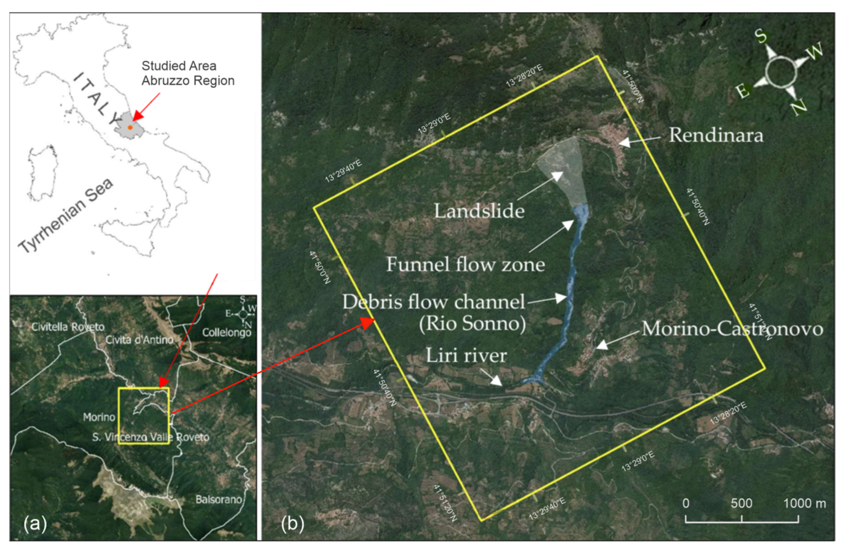
All experiments use the real Morino–Rendinara DEM, but they serve different assessment purposes. The Morino–Rendinara study area is located in the Roveto Valley, Abruzzo Region, Central Italy. Figure 1 provides the national and regional location together with an overview of the slope instability, funnel flow zone, Rio Sonno debris-flow channel, and the downstream connection with the Liri River. Field and UAV documentation of the upper and lower Rio Sonno channel and of the deposits near the Liri River was collected after the event and is reported in the published case-study documentation [13]; those observations provide the geomorphological context for the literature-based parameterization used here.

The first five groups are controlled tests that verify the inversion machinery, evaluate the structure of the objective function, quantify stochastic repeatability, examine observation perturbations, and investigate conditional identifiability. The final two-zone experiment is also a controlled retrieval test, but its reference parameterization is taken from the published RAMMS back-analysis of the real Morino–Rendinara event [13]. For the Morino–Rendinara retrieval experiment, erosion, curvature and inflow effects were intentionally kept deactivated from the solver to preserve consistency with the reference back-analysis configuration being inverted. The objective is to determine whether the published effective friction parameterization can be recovered automatically within the same controlled forward model structure, rather than to construct a new event reconstruction with additional physics. Activating erosion–entrainment, curvature, extra inflow, or other source terms absent from the reference setup would change the forward problem and would mix parameter retrieval error with structural model differences. These literature-based Voellmy coefficients are assigned to two fixed polygons delimiting the two distinct rheological zones in the in-house solver, the resulting final accumulation is then generated on the real terrain, after which the coefficients are treated as unknown and recovered through the inversion. The framework must then recover them from the final thickness field while searching the prescribed parameter intervals. This two-zone test evaluates whether a documented real-event parameterization can be retrieved automatically and reproducibly within the proposed full-flowfield framework.

The assessment comprises six experiments. For Experiments 1–5, which involve the estimation of a single spatially uniform Voellmy–Coulomb coefficient, the inversion domain is fixed to $\mathsf{\mu }\in [0.05,0.60]$, with a configured initial candidate of ${\mathsf{\mu }}_0=0.30$. The same admissible interval is used for the complete one-dimensional objective landscape analysis in Experiment 2. In Experiment 6, the two-zone inversion is instead performed over ${\mathsf{\mu }}_{\mathrm{up}}\in [0.005,0.05]$ and ${\mathsf{\mu }}_{\mathrm{down}}\in [0.05,0.20]$, with configured initial candidate $({\mathsf{\mu }}_{\mathrm{up},0},{\mathsf{\mu }}_{\mathrm{down},0})=(0.03,0.12)$. Experiment 1 evaluates the capability of the complete GA + GD workflow to recover spatially uniform coefficients from reference deposits generated with ${\mathsf{\mu }}_{\mathrm{ref}}\in \{0.10,0.25,0.45\}$. Experiment 2 examines the baseline objective function landscape by sampling $\mathsf{\mu }\in [0.05,0.60]$ using 101 regularly spaced values and additionally including the exact reference value $\mathsf{\mu }=0.25$. This scan separates the total objective from its weighted thickness, support, and signed distance contributions. Experiment 3 assesses the repeatability of the complete stochastic–deterministic pipeline by repeating the baseline inversion with ten random seeds. Experiment 4 investigates robustness to observation perturbations by adding relative Gaussian noise with standard deviations of 5, 10, and 20% to positive thickness values; randomly removing 10, 30, and 50% of the valid observation cells; multiplying the complete observation field by factors of 0.90 and 1.10; and evaluating wet thresholds of 0.001, 0.005, 0.01, 0.05, 0.10, 0.50, and $1.00$ m. The noise and missing cell tests are performed using five independent realizations at each perturbation level. Experiment 5 studies conditional identifiability by fixing $\xi$ at 250, 375, 500, 750, and 1000 m s⁻² while estimating only $\mathsf{\mu }$ from an observation generated with ${\xi }_{\mathrm{ref}}=500 \mathrm{m} {\mathrm{s}}^{-2}$. Experiment 6 is a controlled Morino–Rendinara back-analysis retrieval test: the published values ${\mathsf{\mu }}_{\mathrm{up}}=0.01$ and ${\mathsf{\mu }}_{\mathrm{down}}=0.10$ are assigned to their documented spatial zones on the real terrain, the resulting accumulation field is used as the target, and the coefficients are then recovered by inversion.

For the two-zone Morino–Rendinara retrieval experiment, the valid cells of the reference accumulation raster were randomly partitioned into a calibration subset and a held-out subset, corresponding to approximately 70% and 30% of the valid cells, respectively. The GA+GD inversion and the calibration objective were evaluated using only the calibration mask, whereas the complementary cells were excluded from the cell-wise fitting procedure and reserved for post-optimization assessment. After convergence, the best-fitting simulation was evaluated on the held-out mask using the same full-field objective formulation, together with RMSE and IoU. The resulting held-out metrics therefore provide a spatial out-of-sample diagnostic of how well the recovered coefficients reproduce portions of the reference accumulation field not directly used in the parameter search.

Thickness discrepancies are summarized by the root mean square error (RMSE).

An overview of the complete experiment suite, including the unknown parameters, controlled references, and primary evaluation diagnostics, is provided in

Table 2. Experiment matrix used to evaluate numerical recovery, noise robustness, conditional identifiability, and case-study parameter retrieval.

Experiment	Unknown Parameter(s)	Controlled Reference	Primary Diagnostic
Uniform reference recovery	$\mathsf{\mu }$	${\mathsf{\mu }}_{\mathrm{ref}}=0.10,0.25,0.45$	Parameter error, objective, RMSE, IoU, evaluations
Objective function profile	$\mathsf{\mu }$	${\mathsf{\mu }}_{\mathrm{ref}}=0.25$	Total objective and weighted spatial components
GA+GD repeatability	$\mathsf{\mu }$	Ten independent random seeds	Mean, dispersion, maximum error, success rate
Observation robustness test	$\mathsf{\mu }$	Noise, missing cells, thickness scaling, and wet threshold changes	Parameter bias, RMSE, and IoU under perturbed observations
Conditional $\xi$ test	$\mathsf{\mu }$ with prescribed $\xi$	$(\mathsf{\mu },\xi )=(0.25,500\mathrm{m}{\mathrm{s}}^{-2})$	Compensating relation $\widehat{\mathsf{\mu }}\left(\xi \right)$
Morino–Rendinara controlled back-analysis retrieval	${\mathsf{\mu }}_{\mathrm{up}},{\mathsf{\mu }}_{\mathrm{down}}$	Solver-generated target on real terrain using published values $(0.01,0.10)$ on fixed polygons	Parameter retrieval, held-out fit, residual fields, 2-D objective surface

. All the experiments were executed on an NVIDIA GeForce RTX 5060 Laptop GPU using the production CUDA kernels.

2.6. Evaluation and Identifiability Diagnostics

Parameter recovery is evaluated through the absolute error $|\widehat{\mathsf{\mu }}-{\mathsf{\mu }}_{\mathrm{ref}}|$ and its relative counterpart. Agreement between simulated and reference deposits is evaluated with the complete objective J, thickness RMSE, and wet area intersection over union (IoU). The number of forward objective evaluations is reported as a computational diagnostic. For perturbed observations, parameter and field metrics are interpreted relative to the imposed disturbance rather than against an expectation of zero residual. In the controlled Morino–Rendinara retrieval test, the best inversion is compared with the reference accumulation generated on the real terrain using the published two-zone coefficients.

The selected diagnostics are deliberately broader than a single runout or inundation metric. Runout-based and calibration-based studies remain essential for operational hazard assessment [9,19], but previous work also shows that calibration outcomes depend on both the selected model and the observations used to constrain it. Schraml et al. reported model-dependent Voellmy parameter ranges and sensitivities when back-calculating the same Alpine debris-flow events with RAMMS–DF and DAN3D [21], whereas Calvello et al. demonstrated that the amount and spatial distribution of deposit thickness information can materially affect inverse-analysis reliability [24]. Likewise, field-scale Italian back-analyses indicate that rheological parameters inferred from one information source or event should be transferred cautiously and are better constrained when field and experimental evidence are integrated [20]. These findings motivate the present use of RMSE and IoU together with a composite full-field objective and explicit identifiability diagnostics. The comparison is methodological rather than a claim that one metric is universally superior: the most informative observation depends on data quality, process scale, model structure, and the decision variable of interest.

Optimization accuracy and parameter identifiability are related but distinct. Repeated convergence to the same minimum demonstrates numerical repeatability of the search procedure. Identifiability instead asks whether the observation changes sufficiently and uniquely with the parameter. A parameter can therefore be recovered with high numerical precision while remaining conditional on another parameter or on a particular model structure. Profile-likelihood and sensitivity analyses formalize this distinction by identifying flat or elongated low-misfit regions rather than considering only the best-fitting point [34,35]. For the spatially heterogeneous experiment, substantial overlap between the wet deposit and each prescribed polygon is treated as a necessary, although not sufficient, condition for recovering both zonal coefficients.

3. Results

3.1. Controlled Recovery of a Uniform Friction Coefficient

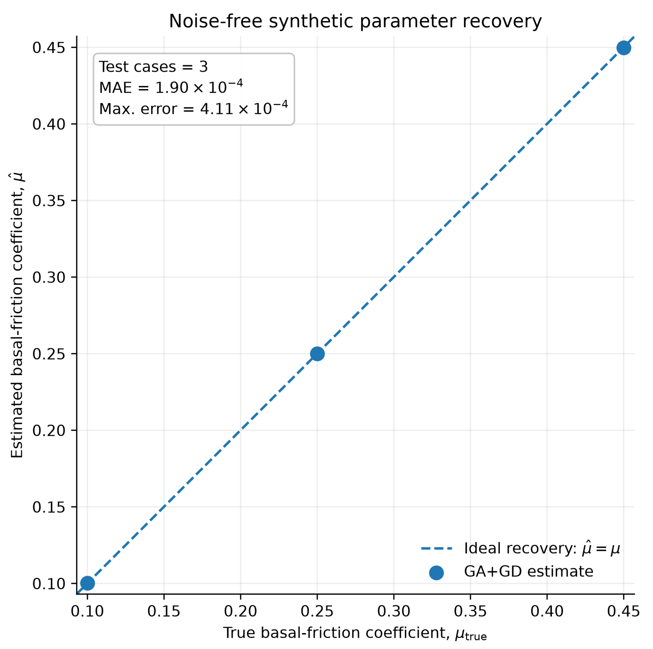
The global–local framework recovered all three uniform reference coefficients with high accuracy (

Table 3. Controlled recovery of the spatially uniform basal friction coefficient. Relative errors are reported as percentages.

${\mathsf{\mu }}_{\mathbf{ref}}$	$\widehat{\mathsf{\mu }}$	Absolute Error	Relative Error (%)	J	RMSE (m)	IoU	Evaluations
0.10	0.100152	$1.52\times {10}^{-4}$	0.1525	$3.42\times {10}^{-8}$	$9.66\times {10}^{-5}$	1.0000	299
0.25	0.249995	$5.39\times {10}^{-6}$	0.0022	$3.81\times {10}^{-13}$	$4.07\times {10}^{-7}$	1.0000	124
0.45	0.449589	$4.11\times {10}^{-4}$	0.0914	$2.36\times {10}^{-11}$	$2.84\times {10}^{-6}$	1.0000	146

; Figure 2). Estimates of 0.100152, 0.249995, and 0.449589 were obtained from reference values of 0.10, 0.25, and 0.45, respectively. Across the three tests, the mean absolute error was $1.90\times {10}^{-4}$ and the maximum absolute error was $4.11\times {10}^{-4}$. The largest relative error, 0.153%, occurred for the lowest coefficient. In every case, the simulated and reference wet footprints coincided exactly, giving IoU equal to one, while thickness RMSE ranged from $4.07\times {10}^{-7}$ to $9.66\times {10}^{-5}$ m.

These controlled results verify the internal consistency of parameter normalization, forward simulation, objective evaluation, global exploration, and local refinement. They define the numerical recovery accuracy attainable when the observation is generated by the same forward model. Robustness beyond this ideal setting is evaluated separately through the observation-perturbation suite.

3.2. Structure of the Full-Flowfield Objective Function

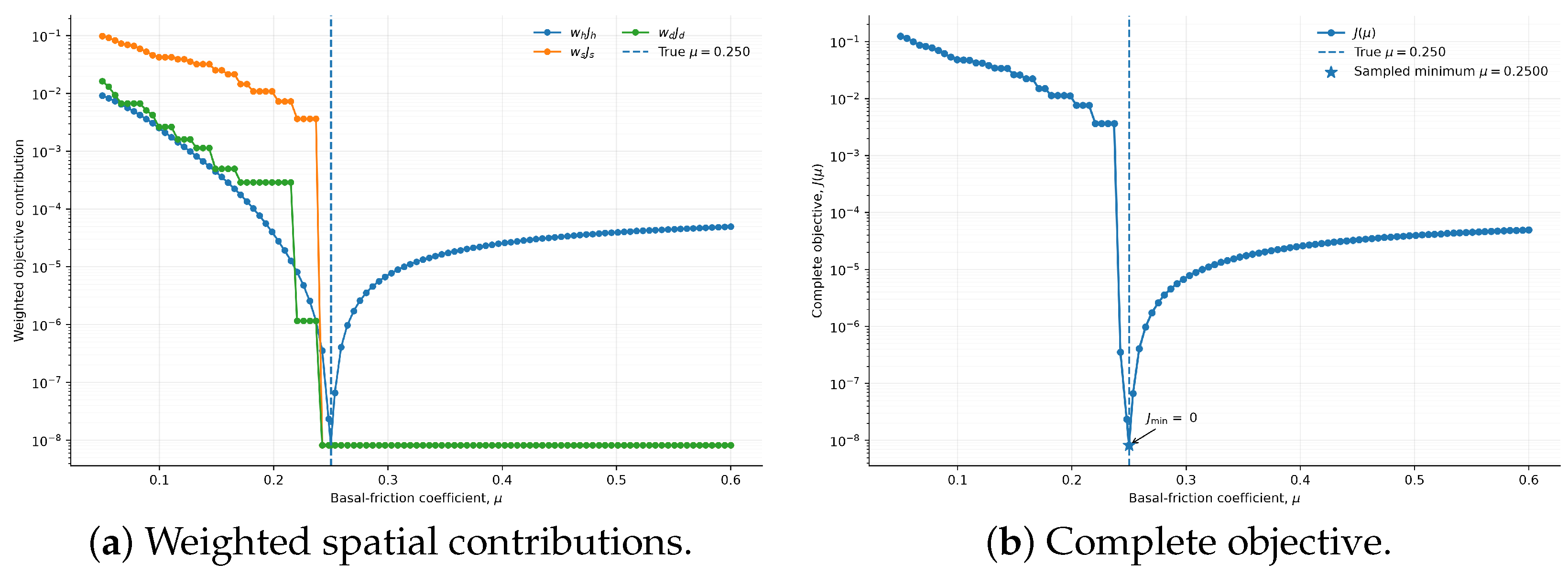
The complete objective function profile has a unique zero at the exact reference coefficient $\mathsf{\mu }=0.25$ (Figure 3). The profile is strongly asymmetric. At $\mathsf{\mu }=0.05$, resistance is too low and the simulated flow is excessively mobile, producing $J=0.12457$, IoU $=0.9010$, RMSE $=0.0596$ m, and a runout excess of approximately 84 m. In this regime, the dominant contribution is $w_s{J}_s$, which penalizes the incorrect wet footprint, while $w_d{J}_d$ also remains substantial because the simulated deposit boundary extends beyond the reference boundary. As $\mathsf{\mu }$ approaches the reference value, both geometric terms fall abruptly to zero when the two wet masks become identical.

For $\mathsf{\mu }\ge 0.2425$ in the sampled profile, IoU is one and both $w_s{J}_s$ and $w_d{J}_d$ are zero. Parameter discrimination is then supplied almost entirely by the weighted thickness term $w_h{J}_h$. The high-friction branch therefore increases gradually: at $\mathsf{\mu }=0.60$, the total objective is only $4.96\times {10}^{-5}$ even though the thickness RMSE has increased to $0.00410$ m. Panel (a) of Figure 3 makes this transition explicit by separating the weighted components, whereas panel (b) shows their combined effect in the total objective J. The objective is consequently not a broad symmetric parabola; it combines a steep geometric penalty for over-mobile solutions with a flatter thickness-controlled branch once the footprint has stabilized.

Representative numerical values from the objective function scan are reported in

Table 4. Selected values from the diagnostic objective function scan. Component columns report the weighted contributions displayed in Figure 3a.

$\mathsf{\mu }$	$\mathit{J}\left(\mathsf{\mu }\right)$	${\mathit{w}}_{\mathit{h}}{\mathit{J}}_{\mathit{h}}$	${\mathit{w}}_{\mathit{s}}{\mathit{J}}_{\mathit{s}}$	${\mathit{w}}_{\mathit{d}}{\mathit{J}}_{\mathit{d}}$	RMSE (m)	IoU	Runout Error (m)
0.0500	$1.2457\times {10}^{-1}$	$9.2170\times {10}^{-3}$	$9.8976\times {10}^{-2}$	$1.6378\times {10}^{-2}$	$5.9570\times {10}^{-2}$	0.9010	84.01
0.2425	$3.5601\times {10}^{-7}$	$3.5601\times {10}^{-7}$	0	0	$3.6163\times {10}^{-4}$	1.0000	0
0.2500	0	0	0	0	0	1.0000	0
0.2700	$1.7240\times {10}^{-6}$	$1.7240\times {10}^{-6}$	0	0	$7.8870\times {10}^{-4}$	1.0000	0
0.6000	$4.9646\times {10}^{-5}$	$4.9646\times {10}^{-5}$	0	0	$4.1032\times {10}^{-3}$	1.0000	0

.

The component-wise analysis explains why a complete thickness raster contains more inverse information than a runout-only target. The support and boundary terms rapidly reject simulations that occupy the wrong cells, while the continuous thickness field continues to distinguish parameter values after the wet footprint has become identical. The exact zero at $\mathsf{\mu }=0.25$ is a property of the controlled forward–inverse experiment and should be interpreted as solver–objective consistency, not as a residual level expected from field observations.

3.3. Repeatability of the GA + GD Inversion

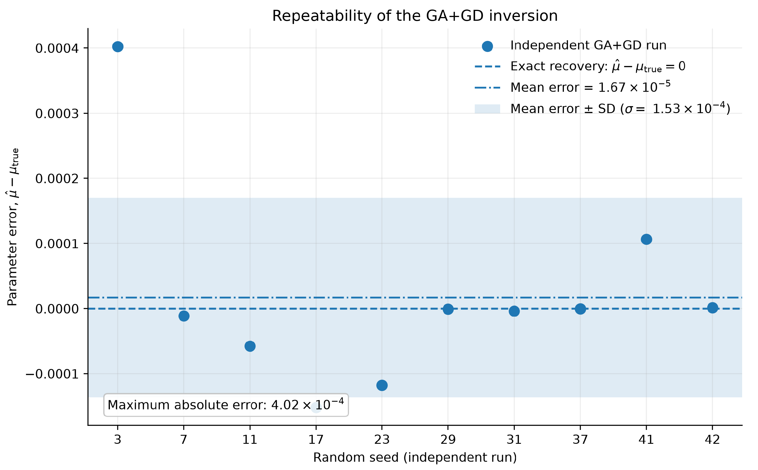
All ten independent inversions converged close to the reference coefficient (Figure 4;

Table 5. Summary of the ten independent baseline inversions.

Diagnostic	Value
Number of runs	10
Reference coefficient	0.250000
Mean $\widehat{\mathsf{\mu }}$	0.250017
Median $\widehat{\mathsf{\mu }}$	0.249998
Sample SD of $\widehat{\mathsf{\mu }}$	$1.53\times {10}^{-4}$
Mean absolute error	$8.52\times {10}^{-5}$
Maximum absolute error	$4.02\times {10}^{-4}$
Mean objective	$1.21\times {10}^{-10}$
Mean evaluations	145.3
Evaluation SD	34.3
Success rate for error $\le 0.01$	100%

). The mean estimate was 0.250017, the sample standard deviation (SD) was $1.53\times {10}^{-4}$, and the median was 0.249998. The mean absolute parameter error was $8.52\times {10}^{-5}$ and the maximum error was $4.02\times {10}^{-4}$. Every run satisfied the success criterion $|\widehat{\mu }-0.25|\le 0.01$. The mean number of objective evaluations was 145.3, with a standard deviation of 34.3.

The small between-run dispersion indicates that the genetic stage consistently located the same low-objective basin and that the local stage refined the solution beyond the resolution of the initial population. This demonstrates repeatability of the optimizer for the tested one-dimensional problem. It does not establish unconditional uniqueness of the physical parameter, as shown by the prescribed-$\xi$ experiment.

3.4. Robustness to Observation Perturbations

The inversion was almost unaffected by random removal of observation cells (

Table 6. Results of the observation-perturbation experiments. Relative thickness noise and missing cell values are means over five independent realizations; baseline and thickness scaling values correspond to individual inversions. The expanded wet threshold row summarizes seven individual inversions spanning 0.001–1.00 m. The reference coefficient is ${\mathsf{\mu }}_{\mathrm{ref}}=0.25$.

Perturbation	Level	$\widehat{\mathsf{\mu }}$ Result	SD ($\widehat{\mathsf{\mu }}$)	Absolute Error	RMSE (m)	IoU
Baseline	–	0.250001	–	$1.38\times {10}^{-6}$	$3.39\times {10}^{-7}$	1.0000
Missing cells	10%	0.250001	$2.05\times {10}^{-8}$	$1.39\times {10}^{-6}$	$3.21\times {10}^{-7}$	1.0000
Missing cells	30%	0.250001	$2.51\times {10}^{-8}$	$1.41\times {10}^{-6}$	$3.07\times {10}^{-7}$	1.0000
Missing cells	50%	0.250001	$2.05\times {10}^{-8}$	$1.39\times {10}^{-6}$	$3.61\times {10}^{-7}$	1.0000
Relative thickness noise	5%	0.251574	0.006957	0.005131	0.00905	0.9985
Relative thickness noise	10%	0.254933	0.016729	0.015198	0.01708	0.9985
Relative thickness noise	20%	0.242234	0.007147	0.008373	0.03242	0.9861
Thickness scaling	0.90	0.234145	–	0.015855	0.01729	0.9963
Thickness scaling	1.10	0.251823	–	0.001823	0.01735	1.0000
Wet threshold	0.001–1.00 m (7 values)	0.250001–0.250005	–	≤5 $\times {10}^{-6}$	$3.39\times {10}^{-7}$–$4.20\times {10}^{-7}$	1.0000 for all thresholds

). The unperturbed baseline recovered $\widehat{\mathsf{\mu }}=0.2500014$, corresponding to an absolute error of $1.38\times {10}^{-6}$. Nearly identical estimates were obtained after removing 10%, 30%, and 50% of valid cells. Even with half of the observation unavailable, the mean estimate remained $\widehat{\mathsf{\mu }}=0.2500014$, the mean absolute parameter error was $1.39\times {10}^{-6}$, and mean IoU remained one. Standard deviations of order ${10}^{-8}$ show that the result was also insensitive to the specific random realization. This robustness arises because spatially distributed random omission leaves substantial redundant information in the full accumulation field. It should not be extrapolated to spatially clustered gaps that remove a diagnostically important part of the deposit.

Relative thickness noise had a clearer influence. At 5% noise, the mean estimate was $\widehat{\mathsf{\mu }}=0.251574$, with mean absolute error 0.005131, mean RMSE $0.00905$ m, and mean IoU 0.9985. At 10% noise, the mean estimate increased to 0.254933 and the mean absolute error reached 0.015198, while mean IoU remained 0.9985. At 20% noise, the mean estimate shifted below the reference value to 0.242234, with mean absolute error 0.008373, mean RMSE $0.03242$ m, and mean IoU 0.9861. Field reconstruction therefore deteriorated progressively with noise, particularly in RMSE and wet area agreement, whereas the parameter error was not monotonic.

The non-monotonic parameter bias under thickness noise is likewise not interpreted as a monotonic physical response of friction to perturbation amplitude. The reversal from positive bias at 5–10% noise to negative bias at 20% arises from the nonlinear interaction among continuous thickness errors, wet threshold crossings, changes in deposit support and boundary position, and the relative weights of the composite objective. The simultaneously high IoU and increased RMSE at 20% noise show that the overall footprint can remain well reproduced even when local thickness amplitudes deteriorate appreciably.

Systematic thickness scaling affected the recovered coefficient more strongly than random missingness. Multiplying the observed field by 0.90 produced $\widehat{\mathsf{\mu }}=0.234145$, an absolute parameter error of 0.015855, and IoU 0.9963. Scaling the field by 1.10 produced $\widehat{\mathsf{\mu }}=0.251823$, an absolute error of 0.001823, and IoU equal to one. The response is therefore asymmetric: a 10% underestimation of thickness had a larger effect on the inferred friction coefficient than an equivalent overestimation. The wet threshold experiment covered 0.001, 0.005, 0.01, 0.05, 0.10, 0.50, and $1.00$ m. Across this three-order-of-magnitude range, the recovered coefficient remained between 0.250001 and 0.250005, with a maximum absolute error of $5\times {10}^{-6}$; IoU was 1.000 for every threshold, the complete objective remained at the numerical floor (approximately $1.75\times {10}^{-13}$ to $4.21\times {10}^{-13}$), and RMSE remained approximately $3.39\times {10}^{-7}$ to $4.20\times {10}^{-7}$ m. Thus, neither the smallest threshold nor the large 0.50–1.00 m thresholds measurably distorted the objective or biased the recovered friction coefficient in this controlled experiment. Taken together, these tests show that the framework is not evaluated only against exact solver-generated observations and that different forms of data uncertainty propagate differently into the inverse estimate (Table 6).

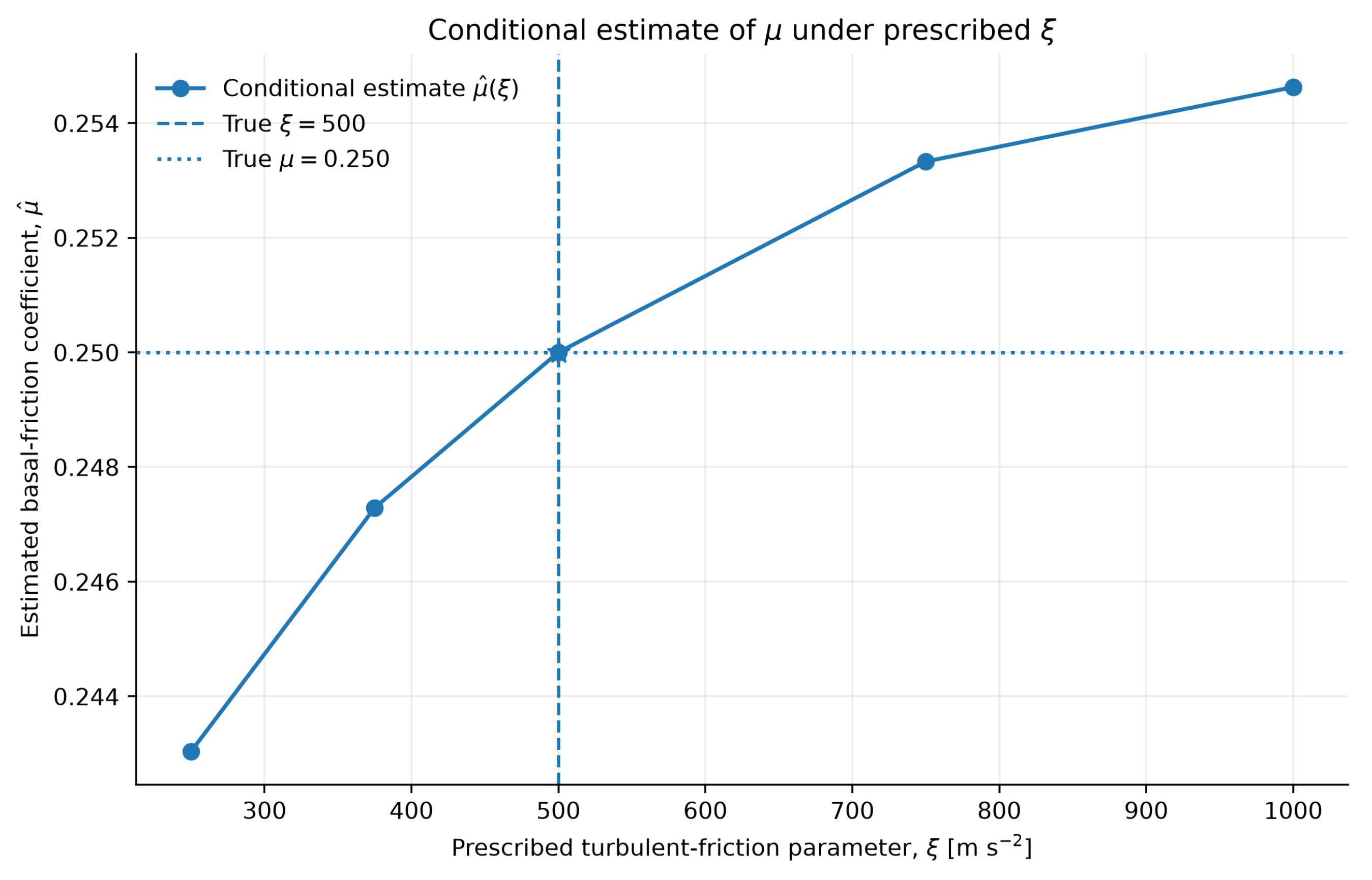
3.5. Conditional Estimate of $\mu$ Under Prescribed $\xi$

The estimated Coulomb coefficient varied monotonically with the prescribed turbulent friction parameter (Figure 5;

Table 7. Conditional recovery of $\mathsf{\mu }$ when $\xi$ is fixed during inversion. The reference observation was generated with ${\xi }_{\mathrm{true}}=500 \mathrm{m} {\mathrm{s}}^{-2}$ and ${\mathsf{\mu }}_{\mathrm{true}}=0.25$.

Prescribed $\mathit{\xi }$ ($\mathbf{m}{\mathbf{s}}^{-2}$)	$\widehat{\mathsf{\mu }}$	Bias in $\mathsf{\mu }$	J	RMSE (m)	IoU	Evaluations
250	0.243038	$-6.962\times {10}^{-3}$	$6.86\times {10}^{-10}$	$1.54\times {10}^{-5}$	1.0000	177
375	0.247289	$-2.711\times {10}^{-3}$	$8.41\times {10}^{-11}$	$5.36\times {10}^{-6}$	1.0000	158
500	0.250001	$1.0\times {10}^{-6}$	$2.69\times {10}^{-13}$	$3.39\times {10}^{-7}$	1.0000	159
750	0.253329	$3.329\times {10}^{-3}$	$8.10\times {10}^{-11}$	$5.28\times {10}^{-6}$	1.0000	167
1000	0.254628	$4.628\times {10}^{-3}$	$2.67\times {10}^{-9}$	$3.20\times {10}^{-5}$	1.0000	167

). Reducing $\xi$ from the reference value of 500 m s⁻² to 250 m s⁻² lowered the estimate to $\widehat{\mathsf{\mu }}=0.243038$. Increasing $\xi$ to 1000 m s⁻² raised the estimate to 0.254628. Across this fourfold range in prescribed $\xi$, the conditional estimate of $\mathsf{\mu }$ spanned approximately 0.0116.

Despite this systematic parameter shift, every simulation retained IoU equal to one and RMSE remained between $3.39\times {10}^{-7}$ and $3.20\times {10}^{-5}$ m. The correct pair produced the smallest objective, but the incorrect prescribed values also generated extremely close field agreement. Thus, the final deposit constrains the combined resistance effect more strongly than it separates the Coulomb and velocity-dependent contributions.

The direction of compensation follows the Voellmy resistance law. Because the quadratic contribution scales as $g{\parallel \mathbf{u}\parallel }^2/\left(\xi h\right)$, reducing $\xi$ increases velocity-dependent resistance and can be offset by reducing the Coulomb contribution $\mu g_n$. Conversely, increasing $\xi$ weakens the quadratic resistance and requires a larger $\mu$ to reproduce a similar final field. The experiment therefore provides a clear example of conditional, rather than joint, identifiability.

3.6. Morino–Rendinara Controlled Back-Analysis Retrieval Test

The Morino–Rendinara experiment is formulated as a controlled back-analysis retrieval test based on the real terrain and on the parameterization documented for the historical event. The event was previously analysed through RAMMS back-analysis and subsequently used for neural operator development [13,14,15]. In this controlled retrieval test, the published reconstruction assigns $\mathsf{\mu }=0.01$ to the upstream region and $\mathsf{\mu }=0.10$ to the downstream region, with $\xi =200 \mathrm{m} {\mathrm{s}}^{-2}$ in both zones and $V=200 {\mathrm{m}}^3$. These documented coefficients define two fixed resistance polygons in the in-house solver; resistance outside the polygons is fixed and is not inverted. The in-house solver first generates the target accumulation on the real Morino–Rendinara DEM, after which the two zonal coefficients are treated as unknown and recovered by inversion. The experiment therefore tests whether the proposed framework can recover the published spatial parameterization without repeating the original manual RAMMS calibration, i.e., whether the documented back-analysis outcome can be reached automatically and reproducibly rather than through subjective trial-and-error.

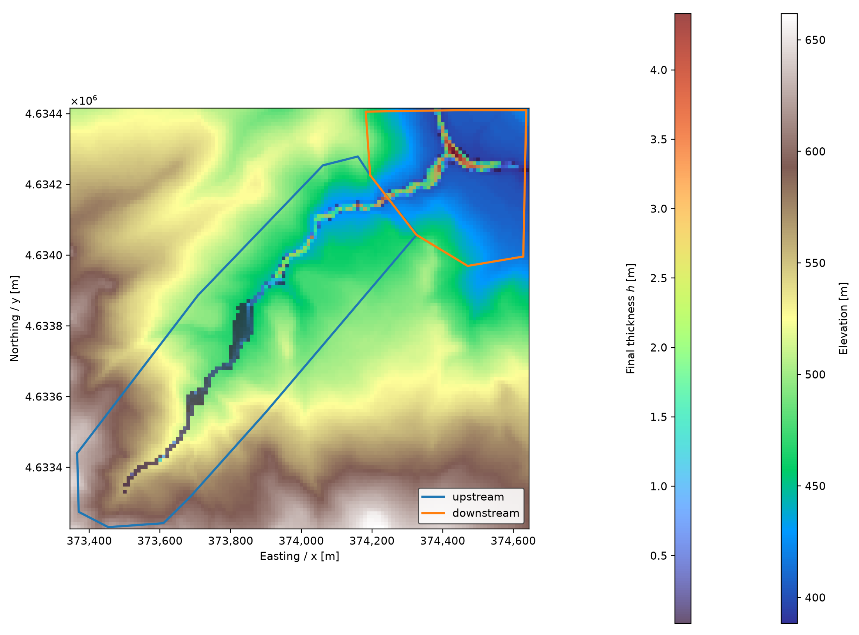
Both resistance zones were substantially sampled by the final deposit (Figure 6). Of the 620 wet cells, 301 cells (48.55%) occurred inside the upstream polygon and 319 cells (51.45%) occurred inside the downstream polygon. The near-balanced distribution provides the spatial excitation required for both coefficients to influence the inverse observation.

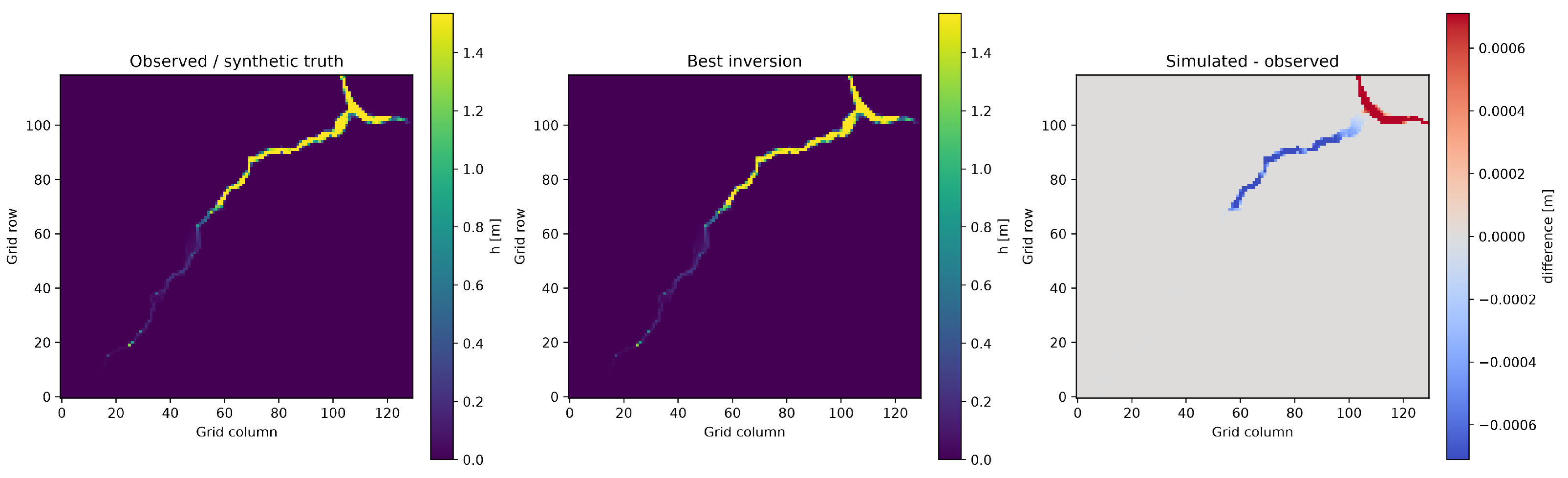
The parameterized two-zone model recovered ${\widehat{\mathsf{\mu }}}_{\mathrm{up}}=0.009991$ and ${\widehat{\mathsf{\mu }}}_{\mathrm{down}}=0.100184$ from reference values of 0.01 and 0.10. The calibration and held-out objectives were $9.8878\times {10}^{-10}$ and $9.7305\times {10}^{-10}$, respectively; held-out RMSE was $4.4902\times {10}^{-5}$ m and held-out IoU was one. The residual fields in Figure 7 confirm that the two coefficients are recoverable when both zones are dynamically sampled and the inverse parameterization is consistent with the reference configuration.

The complete calibration and held-out evaluation metrics are summarized in

Table 8. Two-zone model. The published reference zonal coefficients were ${\mathsf{\mu }}_{\mathrm{up}}=0.01$ and ${\mathsf{\mu }}_{\mathrm{down}}=0.10$.

Model	Parameters	Estimated Coefficient(s)	Calibration J	Held-Out J	Held-Out RMSE (m)	Held-Out IoU	Evaluations
Two-zone	2	${\mathsf{\mu }}_{\mathrm{up}}=0.009991$, ${\mathsf{\mu }}_{\mathrm{down}}=0.100184$	$9.8878\times {10}^{-10}$	$9.7305\times {10}^{-10}$	$4.4902\times {10}^{-5}$	1.0000	226

.

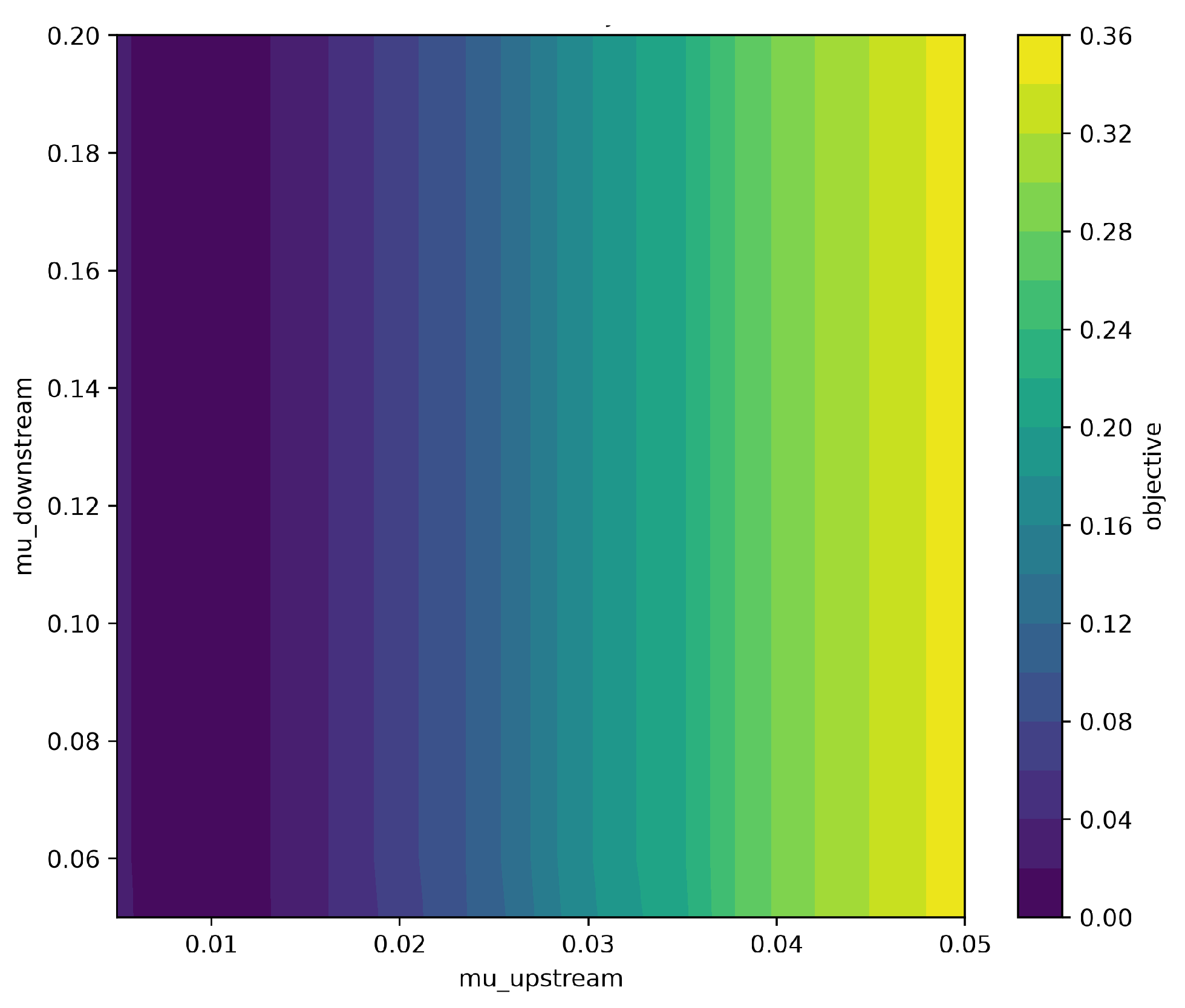
The two-dimensional objective surface is strongly anisotropic (Figure 8). Broad, nearly vertical bands indicate that the objective is more sensitive to the upstream coefficient over much of the sampled domain, which is physically consistent with upstream resistance affecting the flow before it enters the downstream zone. A narrower trough remains visible along the downstream direction. The minimum of the coarse $16\times 16$ diagnostic grid occurs at $({\mathsf{\mu }}_{\mathrm{up}},{\mathsf{\mu }}_{\mathrm{down}})=(0.011,0.08)$ with $J=0.00451$. This point is not the inversion estimate: the true upstream value 0.01 is not a node of the coarse grid, and sparse sampling displaces the apparent minimum along the coupled low-objective valley. The continuous global–local search resolves the narrower basin and recovers $(0.009991,0.100184)$ with objective below ${10}^{-9}$.

4. Discussion

Reliable calibration of debris-flow models is important for reproducible hazard mapping, transparent scenario analysis, and risk-informed territorial planning. The proposed framework addresses this need by replacing subjective trial-and-error adjustment with an explicit forward–inverse workflow and a spatially distributed objective function. Its assessment was deliberately organized as a progression: exact synthetic recovery verified the numerical implementation; repeated inversions evaluated optimizer stability; perturbed observations tested robustness beyond exact model-generated data; conditional inversions exposed parameter compensation; and the published Morino–Rendinara two-zone configuration, implemented on the real terrain, provided a controlled test of whether a documented real-event back-analysis parameterization can be retrieved automatically.

Relative to previous debris-flow calibration and back-analysis studies, the contribution of the present work is primarily in how the inverse problem is posed and documented. Calibration-based forward analyses have traditionally adjusted resistance parameters against event-scale descriptors such as runout, inundation extent, or depositional characteristics [9,19]; the published Morino–Rendinara RAMMS study likewise established a spatially differentiated parameterization through back-analysis of the event [13]. By contrast, the present objective retains the complete final-thickness raster and uses an explicit global–local optimizer to retrieve the coefficients within a fixed forward model structure. The current deterministic framework does not replace those approaches and does not eliminate equifinality; its specific advantage is a reproducible spatial misfit definition combined with controlled tests that expose recovery accuracy, robustness, and compensation effects while reducing computational time.

The practical link to mitigation is indirect but important. The inversion framework is not a structural or non-structural mitigation measure by itself; rather, a reproducibly calibrated forward model can provide a more defensible basis for scenario maps used to evaluate exposed roads, bridges, river crossings, buildings, and other assets. Such calibrated scenarios can support the comparison and prioritization of structural measures, such as channel or retention works, and non-structural measures, such as land-use zoning, emergency planning, monitoring priorities, and civil protection scenarios. The value of the inversion in this context lies in documenting which effective parameters reproduce the available evidence and how sensitive those parameters are to assumptions and observations, so that uncertainty is visible when simulation products are translated into risk-reduction decisions.

4.1. Controlled Verification and Observation Perturbations

The uniform recovery and repeatability tests provide strong evidence of numerical consistency. Across three widely separated reference coefficients, the maximum parameter error was $4.11\times {10}^{-4}$, and ten stochastic repetitions recovered the baseline coefficient with a standard deviation of $1.53\times {10}^{-4}$. The objective function scan independently located the unique minimum at the reference coefficient within the tested interval. These results show that parameter normalization, forward simulation, objective evaluation, global exploration, and local refinement operate coherently as a single inversion framework.

Controlled forward–inverse tests are necessary because they provide known reference parameters and directly measurable recovery errors. However, the forward and inverse calculations in the exact tests share the same equations, discretization, DEM, release condition, and resistance law. Extremely small residuals are therefore expected when model discrepancy is absent, a configuration commonly discussed as an inverse crime [36]. For this reason, exact recovery is treated here as verification of the implementation rather than as sufficient evidence of real-world validity.

The perturbation suite extends the assessment to non-exact observations. Random omission of up to 50% of cells had negligible effect because information remained spatially distributed across the deposit. Thickness noise and systematic scaling had stronger effects because they changed the amplitude information used by $J_h$ and, at higher levels, altered wet–dry classification and boundary geometry. At 20% noise, mean IoU remained 0.9861 and the mean absolute parameter error was 0.008373, indicating useful robustness but also a measurable loss of parameter precision. The results emphasize that observation uncertainty should be represented according to its spatial and physical origin rather than summarized by a single generic noise level.

4.2. Information Supplied by the Full Deposit Field

The objective function profile demonstrates how the four mismatch terms contribute complementary information. For low $\mu$, the simulated deposit extends too far and occupies incorrect cells. In this regime, $w_s{J}_s$ and $w_d{J}_d$ strongly penalize excessive mobility. Once the wet footprints coincide, those geometric terms become zero and the remaining discrimination is provided by $w_h{J}_h$, which measures local thickness differences. The inversion therefore operates in two connected stages: geometrical rejection of incorrect deposit extents and amplitude-based refinement within a common footprint.

This behaviour explains why a complete final-thickness raster is more informative than runout distance or total volume alone. The raster preserves thickness variations throughout the transport and deposition path, which can distinguish simulations that would appear equivalent under a single scalar metric. In inverse problem terms, the approach resembles matching a complete measured field rather than a limited set of attributes [26]. Nevertheless, a large number of pixels does not imply the same number of independent constraints. Adjacent cells are spatially correlated, binary support can remain constant over a parameter interval, and multiple physical parameters can generate nearly identical fields. Full-flowfield inversion increases the available information but does not eliminate non-uniqueness.

The hard wet threshold is also responsible for non-smooth changes in the support and boundary terms. The GA is effective for locating the appropriate basin despite these discontinuities, while finite-difference local refinement exploits the smoother thickness response near the optimum. In the sensitivity test, thresholds from 0.001 to 1.00 m produced effectively identical inverse estimates and IoU equal to one. This invariance is specific to the controlled near-exact recovery setting, because changing the threshold selects matching contour levels of two almost identical rasters. In direct field applications, objective weights and wet thresholds should be linked to survey uncertainty, minimum detectable thickness, spatial resolution, and the hazard quantity of interest rather than selected only for numerical sharpness.

4.3. Conditional Identifiability and Resistance Compensation

The prescribed-$\xi$ experiment provides the clearest evidence that a precise inverse estimate can remain conditional on another parameter. All five inversions reproduced the wet footprint exactly and achieved very small RMSE values, yet $\widehat{\mathsf{\mu }}$ changed systematically as $\xi$ was varied. Both coefficients oppose motion, and their effects can partially compensate along a specific trajectory. The final deposit consequently constrains an effective integrated resistance more strongly than it separates the Coulomb and velocity-dependent mechanisms.

This behaviour is a form of practical non-identifiability, which appears geometrically as an elongated low-objective direction in parameter space [34]. Related anisotropic sensitivities are often described as parameter sloppiness: model outputs can be reproduced accurately even though individual parameters are only weakly separated [35]. The present conditional experiment does not prove structural non-identifiability of the complete $(\mathsf{\mu },\xi )$ pair, because the correct prescribed $\xi$ still gives the lowest objective and a joint two-parameter inversion was not performed. It does show, however, that final accumulation alone provides limited information on how total resistance is partitioned between the two Voellmy terms.

A full joint inversion of $\mathsf{\mu }$ and $\xi$ is a planned methodological extension of the present study. Joint estimation of $\mathsf{\mu }$ and $\xi$ will require observations with different sensitivities to frictional and velocity-dependent resistance. Arrival times, front trajectories, velocity measurements, dynamic pressure, time-resolved thickness, or multiple events with contrasting depth and speed are promising additions because the quadratic term depends explicitly on ${\parallel \mathbf{u}\parallel }^2/h$. Profile likelihoods, multidimensional objective surfaces, or Bayesian posterior distributions should accompany future joint inversions so that compensating valleys are reported rather than hidden behind a single optimum. Bayesian active learning strategies may also reduce the number of expensive forward simulations required for uncertainty characterization [25].

4.4. Spatial Heterogeneity, Zone Excitation, and Parsimony

The controlled Morino–Rendinara two-zone comparison tests a heterogeneous parameterization derived from a documented real-event back-analysis. Both zones are well sampled: 48.55% of the final wet cells occur in the upstream polygon and 51.45% in the downstream polygon. Under these conditions, the two-zone inversion recovers the published coefficients and reproduces the held-out accumulation at near machine precision.

The stronger global sensitivity to ${\mathsf{\mu }}_{\mathrm{up}}$ is physically reasonable because upstream resistance affects the flow history before the mass enters the downstream region. The downstream coefficient remains recoverable because a large portion of the moving material crosses that polygon and the final deposit changes measurably in response. This leads to an important design principle: spatial parameters can only be inferred where the event excites the corresponding zones and where the selected observations retain sensitivity to their effects.

Heterogeneous parameterization should therefore follow a parsimony-first strategy. Zones should be justified by mapped differences in terrain, substrate, confinement, material, or process conditions; their dynamic excitation should be quantified before inversion; and the heterogeneous model should be compared with a simpler alternative on independent data. Objective surfaces, profiles, or sensitivity diagnostics should also be examined for flat or coupled directions. Previous debris-flow studies have emphasized that effective resistance parameters depend on rheology and event conditions and may not transfer directly between sites or releases [9,19]. The present results further show that recoverability varies within a single event according to the path sampled by the flow.

4.5. Role and Computational Cost of the Global–Local Optimizer

The global and local stages perform complementary tasks. The genetic algorithm provides bounded exploration and reduces dependence on the initial guess, whereas projected finite-difference descent resolves the optimum more precisely than a practical diagnostic grid. This distinction is particularly evident in the two-zone test: the coarse $16\times 16$ surface identifies the correct low-friction region but does not locate the continuous optimum, while GA + GD recovers both reference coefficients.

Computational cost remains manageable for the present low-dimensional tests but will become important in joint, spatial, or uncertainty-aware inversions. Increasing the number of parameters, evaluating multiple release or DEM realizations, or sampling a posterior distribution would multiply this cost. A validated neural operator surrogate could further optimize and accelerate the inversion framework, improving computational efficiency while preserving predictive accuracy. From this perspective, both the forward model evaluation and the inversion procedure itself could be enhanced through deep-learning techniques and neural operators, with the aim of reducing computational cost and enabling faster exploration of the parameter space. Such a future strategy would connect the inverse framework with the previously developed fast forward operators [14,15], while keeping surrogate error distinct from observation and structural model uncertainty.

4.6. Limitations and Next Steps

Several limitations define the interpretation of the present results. First, only $\mathsf{\mu }$ is inverted in the uniform experiments, while the analysis of $\xi$ is conditional rather than joint. The framework therefore demonstrates parameter recovery and compensation but does not yet quantify the complete two-parameter uncertainty structure. A dedicated joint $\mathsf{\mu }$–$\xi$ study should examine multidimensional objective surfaces, profile likelihoods, and/or Bayesian posterior distributions.

The current optimization returns deterministic point estimates. Confidence intervals are not yet reported. Future work should quantify uncertainty through profile likelihood, spatial bootstrap procedures, ensemble perturbations, or full Bayesian inversion [37]. Bayesian sampling would provide posterior distributions and parameter correlations but would substantially increase the number of forward evaluations.

The constant-density formulation represents a deliberate simplification of the present forward model, consistent with the controlled inversion framework adopted in this study. This assumption enables the effects of the selected Voellmy resistance parameters to be isolated and their recoverability to be assessed without introducing additional sources of non-uniqueness. In natural debris flows, however, bulk density may evolve spatially and temporally as a consequence of variations in water content, sediment concentration, entrainment, deposition, or mixture composition. Extending the framework to variable-density or variable-composition formulations would therefore represent a valuable subsequent development, although it would also introduce additional parameters and interactions that may increase the complexity of the inverse problem. Similarly, erosion–entrainment, evolving topography, curvature effects, and additional inflow are intentionally excluded from the present retrieval experiments in order to remain consistent with the reference back-analysis configuration and to provide a controlled assessment of parameter recovery. Their progressive inclusion represents a natural extension toward increasingly realistic field applications.

An additional aspect concerns the selection of the objective function weights. In the present study, the weights were defined a priori and kept unchanged throughout the complete experiment suite, providing a consistent basis for comparing the different retrieval and robustness tests. A formal weight sensitivity or weight optimization analysis was not undertaken because it was outside the scope of the present work. Consequently, the adopted values should be regarded as a practical configuration for the proposed controlled experiments rather than as universally optimal coefficients. In future field applications, their definition could be further tailored to problem-specific information, including survey uncertainty, raster resolution, minimum detectable deposit thickness, and the quantity of greatest interest.

The Morino–Rendinara experiment should also be interpreted within the specific objective of the present study. It constitutes a controlled retrieval of a documented back-analysis parameterization over real terrain rather than a direct inversion of raw field observations. This design provides an important intermediate test between fully synthetic experiments and field-scale inversion, because it allows the ability of the proposed optimization framework to recover a previously established spatial parameterization to be assessed under realistic topographic conditions while retaining a known reference solution. A subsequent field application represents the natural next step and could explicitly incorporate additional sources of uncertainty, including measurement error, terrain uncertainty, thin-deposit detection limits, and structural model discrepancy.

The random-cell removal experiments provide encouraging evidence of robustness to substantial amounts of randomly missing observations. These results, however, do not necessarily imply an identical response to spatially clustered data gaps, because removing a contiguous portion of the deposit may eliminate correlated information on runout extent, boundary geometry, and local thickness simultaneously. This represents a different and potentially more demanding observation scenario rather than a limitation of the random-removal analysis itself. Spatial block removal and clustered observation gaps are therefore identified as useful extensions of the present robustness assessment. In particular, future developments will include validation against real observational datasets together with tests based on spatially connected missing data clusters, thereby providing a closer representation of realistic patterns of incomplete field observations.

Finally, future validation should combine final accumulation with time-dependent information, use spatial block holdout tests, jointly estimate $\mu$ and $\xi$, and compare the recovered parameters across multiple events. These developments are necessary before effective friction coefficients are interpreted as transferable predictive quantities rather than event- and model-conditional calibration parameters.

5. Conclusions

This study developed a global–local full-flowfield inversion framework for estimating effective debris-flow resistance parameters from final accumulation rasters. By coupling a conservative two-dimensional finite-volume solver with GA-based global exploration and projected finite-difference gradient descent, the approach replaces manual trial-and-error calibration with a bounded and reproducible optimization procedure. The composite objective retains complementary information from deposit thickness, wet area support, boundary position, and total volume.

The controlled experiments verified the internal consistency and numerical repeatability of the complete forward–inverse workflow. Uniform reference values $\mathsf{\mu }=0.10$, 0.25, and 0.45 were recovered with a mean absolute error of $1.90\times {10}^{-4}$, while all reconstructed wet footprints achieved IoU equal to one. Ten independent baseline inversions converged to the same minimum with a standard deviation of $1.53\times {10}^{-4}$ and a 100% success rate. The perturbation experiments showed that spatially random removal of up to 50% of observation cells had negligible influence because substantial information remained distributed across the accumulation field. Thickness noise and systematic amplitude errors were more influential; nevertheless, at 20% relative noise, the mean IoU remained 0.9861 and the mean absolute parameter error was 0.008373.

The results also demonstrate that numerical precision does not imply unconditional physical identifiability. When $\xi$ was prescribed between 250 and 1000 m s⁻², the estimated $\mathsf{\mu }$ varied from 0.243038 to 0.254628 even though the corresponding final fields remained extremely similar. Final accumulation therefore constrains the integrated resistance more strongly than it separates the Coulomb and velocity-dependent Voellmy contributions. In the controlled Morino–Rendinara back-analysis retrieval test, both resistance regions were dynamically sampled and the framework recovered ${\mathsf{\mu }}_{\mathrm{up}}=0.009991$ and ${\mathsf{\mu }}_{\mathrm{down}}=0.100184$, reproducing the held-out reference accumulation with an RMSE of $4.49\times {10}^{-5}$ m and IoU equal to one. This result shows that spatially heterogeneous coefficients can be recovered when the parameterization is consistent with the reference model and the reference flow path excites each zone. It should not be interpreted as an independent validation against raw field data.

Overall, within the controlled experiments and the single Morino–Rendinara retrieval test considered here, full-flowfield inversion provides a transparent and reproducible route to event back-analysis because it retains more spatial information than runout- or volume-only objectives. This result should not be generalized as evidence of universal performance across debris-flow types, terrains, or observation systems. The recovered coefficients should, however, be interpreted as event-, data-, and model-conditional effective parameters. Future developments should jointly estimate $\mathsf{\mu }$ and $\xi$, incorporate time-dependent observations, quantify uncertainty through profile likelihoods or Bayesian inference, test spatially clustered data gaps, and compare calibrated parameters across multiple independent events before assessing their predictive transferability. These extensions should include direct inversion of raw field observations with explicit treatment of measurement and terrain uncertainty and direct visualization of multidimensional objective surfaces. Validated neural operator surrogates will also be investigated as a future strategy for accelerating repeated forward evaluations and parameter-space exploration, while explicitly quantifying surrogate error against the conservative finite-volume solver.