Seismic Fragility Assessment of Jointed Rock Slope Using Incremental Dynamic Analysis and Field-Characterized Barton–Bandis Parameters

Abstract

This study presents a probabilistic seismic fragility assessment of a jointed rock slope by integrating field characterization, incremental dynamic analysis (IDA), and numerical modeling. Dominant joint sets are identified through field mapping, and key discontinuity parameters are estimated for the Barton–Bandis non-linear shear strength criterion. Dynamic simulations are performed using the distinct element method with the continuously yielding (C-Y) joint model to capture progressive shear degradation. Twenty real earthquake ground-motion records are scaled incrementally to perform IDA, with critical block displacement and cumulative joint slip adopted as engineering demand parameters (EDPs). A probabilistic seismic demand model (PSDM) is developed to correlate peak ground acceleration (PGA) with EDPs. Kinematic analysis indicates that planar failure along joint set 1 is the most likely failure mechanism (90% probability), followed by wedge failure along the intersection of joint sets 1 and 2 (52%). Fragility curves are derived for three displacement-based damage states: minor (1 cm), moderate (5 cm), and severe (15 cm). The results demonstrate that seismic deformation is strongly controlled by discontinuity geometry and progressive joint slip, with the slope exceeding the severe damage state at PGA levels as low as 0.4 g, indicating high seismic vulnerability. This highlights the importance of integrating field characterization with dynamic numerical modeling for reliable seismic stability assessment of such discontinuous rock mass. Future work should incorporate larger datasets, in situ testing, and 3D modeling to enhance assessment reliability.

1. Introduction

The seismic stability of jointed rock slopes is a critical concern for infrastructure development in tectonically active regions. In such an environment, repeated dynamic loading may progressively degrade the strength of rock mass [1,2]. The Himalayan Mountain belt, one of the youngest and tectonically active mountain ranges in the world, is characterized by frequent seismic activity leading to intense geological deformation. Therefore, the Himalayan region is highly vulnerable to earthquake-induced geological hazards [3]. Rapid infrastructure development in this region, including hydropower, roadways, and other critical facilities, requires large-scale rock-slope excavation. Such excavation exposes existing discontinuities within the rock mass, thereby increasing the susceptibility of the rock slope to instability. Therefore, the dynamic failure behavior of rock slopes composed of jointed rock mass under seismic loading has become a key research focus [4].

The traditional approach for evaluating the seismic stability of rock slopes predominantly relies on deterministic methods, such as pseudo-static limit equilibrium analysis, is quantify slope stability using a factor of safety (FoS) [5]. While the method is useful for preliminary design and screening assessment, it fails to account for uncertainties associated with seismic loading, the heterogeneity of rock mass, and modeling assumptions [6]. Consequently, a deterministic approach provides limited information regarding the probability of failure or the performance of slopes under seismic loads of varying amplitude and frequency [7]. In particular, the method neglects record-to-record variability in earthquake ground motion, which is a key factor influencing the seismic response and thus limits its applicability for risk-informed design and hazards mitigation [8].

To address this limitation, the rock engineering community is increasingly adopting a performance-based earthquake engineering (PBEE), which establishes a probabilistic relationship between seismic hazard, structural demand, and system capacity [9]. Within this framework, incremental dynamic analysis (IDA), originally proposed by Vamvatsikos and Cornell [10], has emerged as a rigorous computational approach for evaluating the non-linear response of systems subjected to progressively increasing seismic intensities. In IDA, a numerical model is subjected to a set of ground-motion records scaled to multiple intensity levels, which allows response of the system to be evaluated over a wide range of seismic demands [11]. The procedure generates a comprehensive dataset that captures variability in system response arising from record-to-record differences in earthquake characteristics [12]. The resulting dataset forms the basis for developing probabilistic seismic demand models and fragility curves, which quantify the conditional probability of exceeding predefined damage states for given intensity measure (IM) [13]. Although IDA and fragility analysis are well-established in structural engineering, their application to structurally controlled rock slopes remains relatively limited [14].

A significant challenge in extending probabilistic seismic assessment to rock slopes in jointed rock mass lies in the accurate representation of rock joint behavior within numerical models. The seismic response of jointed rock mass is governed by the shear behavior of discontinuities, which is non-linear and dependent on normal stress conditions [15]. The Barton–Bandis (B–B) model is widely recognized for its ability to represent the behavior of rock joints using parameters such as joint roughness coefficient (JRC), joint compressive strength (JCS), and basic friction angle (${\varphi }_b$) [16]. However, many existing numerical studies rely on generalized or assumed joint parameters rather than field-derived values. Such simplifications may fail to accurately represent the in situ behavior of large-scale rock mass, where scale effects, weathering, and spatial variability significantly influence joint properties [17]. The use of uncalibrated/assumed parameters can therefore introduce substantial uncertainty into numerical simulations and reduce the reliability of achieved fragility assessment results [8].

In addition to uncertainties associated with property joints, the representation of seismic input motion also plays a critical role in probabilistic seismic analysis [11]. Many studies evaluating the seismic performance rely on synthetic or artificially generated ground motions, which may not fully reproduce the complex frequency content, duration, and non-stationary characteristics of real earthquake records [18,19,20]. The use of recorded earthquake time histories is therefore essential for capturing realistic record-to-record variability in seismic loading [21]. Moreover, previous fragility studies often treat modeling uncertainty, ground-motion variability, and capacity thresholds separately or in a simplified manner, which may lead to overconfident estimates of seismic risk. Consequently, there is a clear need for an integrated approach that combines field-characterized rock mass joint properties with real earthquake ground-motion records within an IDA-based probabilistic framework.

In response to these challenges, this study presents an integrated framework to assess the seismic fragility of a structurally controlled jointed rock slope. The approach presented here introduces three key findings that address limitations in previous studies.

First, unlike previous works that assume generalized joint properties, this study provides extensive field characterization of Barton–Bandis joint parameters. Second, while many existing studies rely on synthetic ground-motion and pseudo-static analysis, we use real-time-history records as dynamic input for incremental dynamic analysis. Third, instead of treating uncertainty in a simplified way, the study provides a comprehensive uncertainty analysis within the IDA framework.

The numerical analysis is implemented using the universal distinct element code (UDEC), which allows explicit representation of block interactions within a discontinuous rock mass. Field-derived joint properties are incorporated into the model using a continuously yielding (C-Y) joint model [22] to simulate the non-linear dynamic shear behavior of rock joints during seismic loading. The resulting IDA database is then used to develop probabilistic seismic demand relationships and fragility curves. These outputs provide quantitative insight into the seismic vulnerability of structurally controlled rock-slope failures in earthquake-prone mountainous regions.

2. Study Area and Geological Characterization

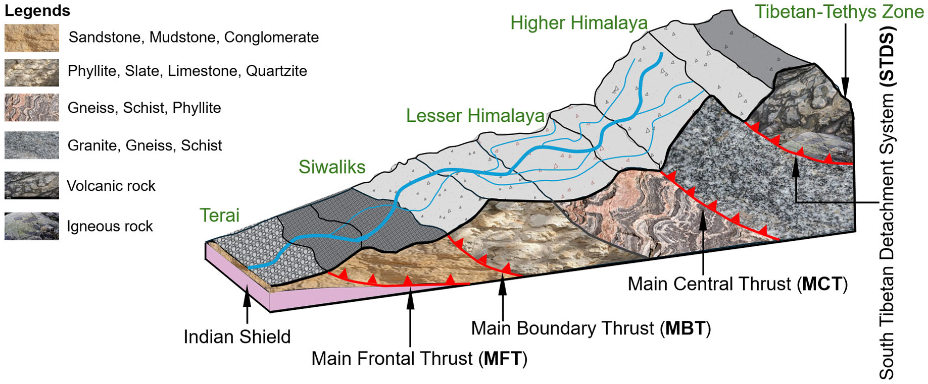
The Himalaya was formed by the collision between the Indian and Eurasian plates. Figure 1 shows the major litho-tectonic zones of the Himalayan orogen, which are separated by a series of regional-scale thrust systems. From south to north, the Siwalik Zone consists of a thick sequence of young sedimentary rocks and is bounded between the Main Frontal Thrust (MFT) to the south and the Main Boundary Thrust (MBT) to the north. The Lesser Himalayan Zone is bounded by the MBT and Main Central Thrust (MCT) to the north. This zone mainly consists of folded and faulted sedimentary and low-grade metamorphic rocks. The Higher Himalayan Zone lies above the MCT and is characterized by high-grade metamorphic and igneous rocks. The Tibetan-Tethys Zone occurs north of the Higher Himalaya and is composed predominantly of fossiliferous marine sedimentary rocks [23].

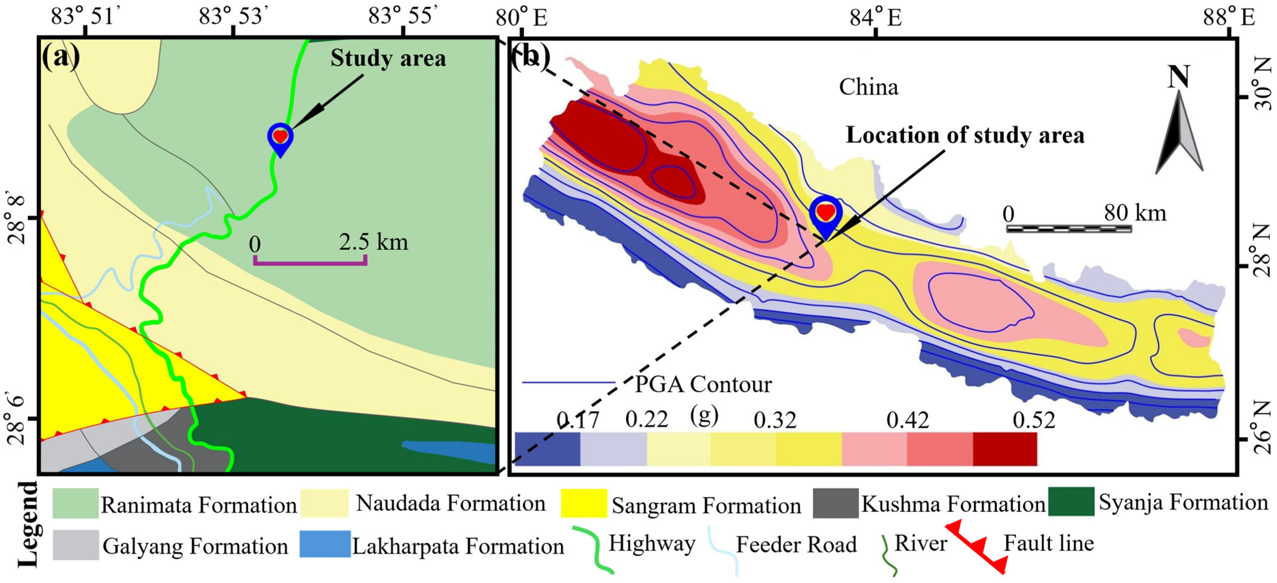
The study area is located at Bhalupahad, approximately 27 km from Pokhara along the Pokhara–Butwal national highway, at coordinates of 28°09′ N and 83°57′ E within the Lesser Himalaya. As shown in Figure 2a, the lithology in this area belongs to the Ranimata Formation of the Lesser Himalayan Zone. This formation consists predominantly of greenish-gray, fine-grained, foliated phyllite interlayered with quartzite and metasandstone layers. Although metasandstone exhibits relatively high strength, it is fractured and jointed, which is a characteristic feature of Lesser Himalayan geology (Class I behavior) [23]. This area is seismically influenced due to its proximity to the MBT. Consequently, the impact of seismic loading on rock-slope failure has a considerable influence (Figure 2b) [25]. Field mapping carried out has identified two major joint sets and the occasional occurrence of random joints in the rock mass.

Table 1. The attitudes of the rock-slope face and joint sets are observed from detailed field mapping.

Rock Slope	Dip (°)	Dip-Direction (°)
Slope face	Mean = 65.34, SD = 4.25	Mean = 200.45, SD = 5.45
Joint Set 1	Mean = 55.15, SD = 6.35	Mean = 205.47, SD = 8.25
Joint Set 2	Mean = 70.65, SD = 6.75	Mean = 341.35, SD = 7.50

presents the statistical distribution of the orientations of the rock-slope face and mapped discontinuity orientations obtained from field mapping. A total of 50 measurements indicate two dominant joint sets, whose orientations follow a normal distribution defined by their mean values and standard deviations.

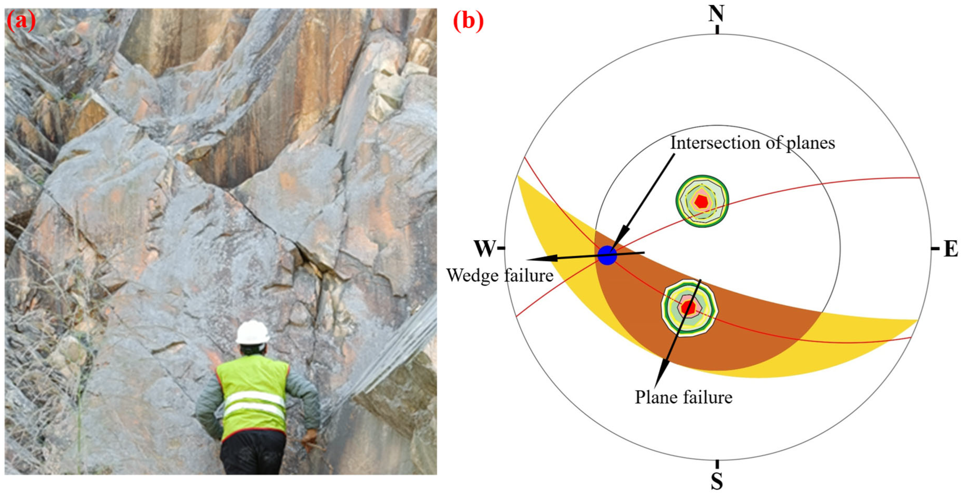
Discontinuity orientation data are analyzed using a lower hemisphere equal area stereographic projection to identify dominant joint sets and assess their structural relationship with the rock-slope face. The pole distribution reveals two distinct clusters representing two major joint sets (Figure 3b). The mean orientations and associated standard deviations of these sets are determined through statistical analysis of the measured attitudes. Kinematic analysis indicates that plane failure is possible along joint set 1, as its mean orientation satisfies the geometric conditions for plane failure relative to the slope face. In addition, wedge failure may occur along the line of intersection between the two joint sets. Wedge failure occurs when the line of intersection of two joints dips out of the slope face at an angle less than the friction angle of the joint surfaces [26].

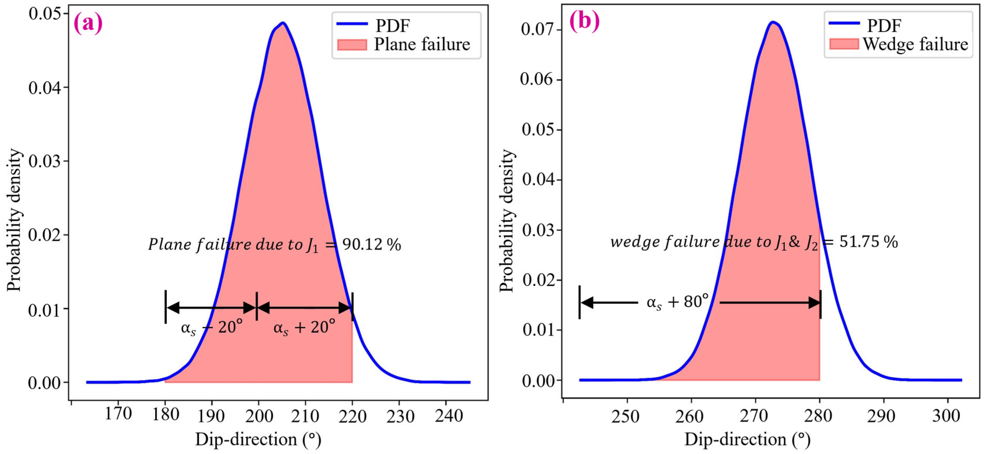
A total of 200,000 realizations are generated using Monte Carlo simulations to estimate the probability of failure (PoF), considering the statistical variability of discontinuity orientations derived from field measurements. The orientation data obtained from 50 measurements are characterized using their mean values and standard deviations. The normality of the dataset is verified using the Shapiro–Wilk test, which yielded p-values greater than 0.05 for all joint sets. Hence, a normal distribution is assumed to represent the variability within each joint set. The kinematic condition for plane failure is expressed as $\varphi < {\Psi }_j < {\Psi }_s$, where $\varphi$ is the friction angle, ${\Psi }_j$ is the dip of the joint set, and ${\Psi }_s$ is the dip of the slope face. The dip-direction constraint is defined as ${\alpha }_s-{20}^{°}\le {\alpha }_j\le {\alpha }_s+{20}^{°}$, where ${\alpha }_s$ is the dip-direction of the slope face and ${\alpha }_j$ is the dip-direction of the joint set. Similarly, the kinematic condition for wedge failure is expressed as $\varphi < {\Psi }_i < {\Psi }_s$, where ${\Psi }_i$ is the dip of the line of intersection due to two joint sets. The dip-direction constraint is defined as ${\alpha }_s-{80}^{°}\le {\alpha }_i\le {\alpha }_s+{80}^{°}$, where ${\alpha }_i$ represents the dip-direction of the line of intersection between the joint sets.

The results indicate that plane failure along the joint set 1 represents the dominant kinematically failure mode for this rock-cut slope, with a probability of failure of 90% (Figure 4a). In addition, wedge failure is also possible along the intersection of joint Set 1 and joint Set 2. Based on the simulation results, the probability of wedge failure is about 52% (Figure 4b).

3. Materials and Methods

3.1. Field Characterization of Joint Properties

The engineering geological properties of the discontinuities are characterized based on detailed field mapping of the exposed joint surfaces within the rock-slope mass. The joint roughness coefficient (JRC) is estimated from the asperity amplitude of the mapped joint surfaces. The correlation chart proposed by Barton and Choubey [27] is used to estimate the JRC of the dominant joint sets. The joint compressive strength (JCS) of the joint wall is estimated from in situ tests using a Schmidt hammer. A Schmidt hammer (L-Type) is employed to obtain rebound values from representative joint surfaces. The rebound numbers are subsequently converted to the joint wall compressive strength using the empirical correlation chart proposed within the Barton–Bandis (B–B) shear strength criterion framework. The obtained JRC and JCS values are used as input parameters in the B–B non-linear shear strength model to characterize the engineering geological behavior of the rock joints. Among these parameters, JRC is considered one of the most influential factors controlling the shear strength of discontinuities [28].

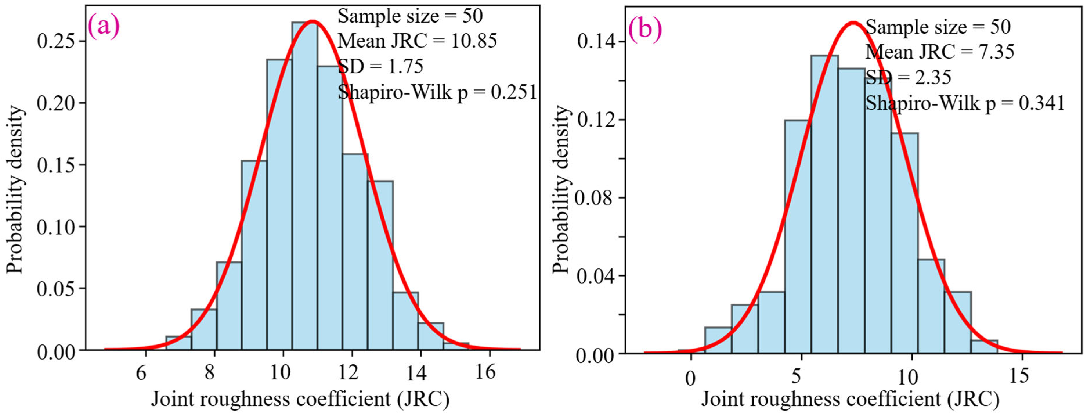
A total of 50 JRC measurements are obtained from extensive field mapping of the dominant joint surfaces. The statistical distribution of JRC values for joint set 1 is presented in Figure 5a. The results indicate that the JRC values follow an approximately normal distribution with a mean value of 10.85 and a standard deviation of 1.75. Similarly, Figure 5b shows that JRC values for Joint set 2 also follow an approximately normal distribution. The normality of the datasets for both joint sets is verified using the Shapiro–Wilk test, which yielded a p-value of 0.251 and 0.341, respectively, which indicate that the assumption of normal distribution is logical.

3.2. Non-Linear Barton–Bandis Failure Criterion

The shear strengths of rock joints are estimated using the non-linear shear strength criterion proposed by Barton [29]. The peak shear strength of a discontinuity is expressed by Equation (1).

$$\tau ={\sigma }_{n}tan\left[JRC {log}_{10}\left({\displaystyle \frac{JCS}{{\sigma }_n}}\right)+{\varphi }_r\right]$$

(1)

where $\tau$ is the peak shear strength, ${\sigma }_n$ is the effective normal stress, ${\varphi }_r$ is the residual friction angle, $JRC$ is the joint roughness coefficient, and $JCS$ is the joint wall compressive strength. These parameters are estimated from field mapping and laboratory testing. For weathered surfaces, the residual friction angle is adopted and estimated following Barton and Choubey [27].

3.3. Limit Equilibrium Analysis for Wedge (Biplane) Failure

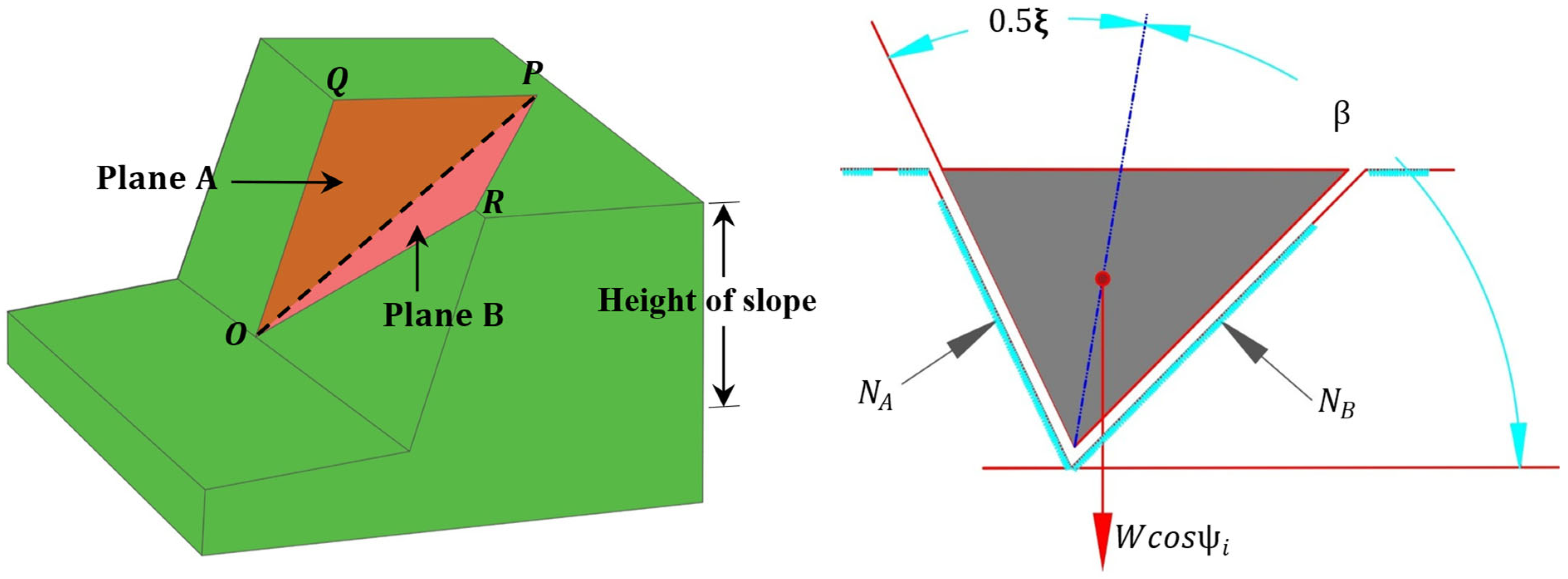
Limit equilibrium analysis is performed to validate the numerical model results under static and dynamic loading conditions [5]. The factor of safety (FoS) is widely used to quantify the stability condition of jointed rock slopes. It is defined as the ratio of resisting (stabilizing) force to driving (sliding) force along the potential failure plane [5]. The FoS is calculated for biplane failure following Jiang and Liu [30] using Equation (2), where $N_A$ and $N_B$ are effective normal reactions and $c_A{A}_A$ and $c_B{A}_B$ are the cohesive forces on plane $A$ and $B$, respectively, and $\overrightarrow{R}$ is the active resultant force. The geometry of biplane failure is shown in Figure 6. These results are used as basis for calibrating numerical modeling.

$$FoS={\displaystyle \frac{N_{A}tan{\varphi }_A+N_{B}tan{\varphi }_B+c_A{A}_A+c_B{A}_B}{\left|\overrightarrow{R}.(\widehat{n_a }x\widehat{ n_b)}\right|/\left|(\widehat{n_a }x\widehat{ n_b)}\right|}}$$

(2)

3.4. Numerical Modeling

The seismic response of the jointed rock slope is investigated using the distinct element method (DEM), a discontinuous modeling approach well-suited for rock mass where mechanical behavior is governed by pre-existing discontinuities [31]. Numerical simulations are conducted using the UDEC, Version 5.0 [22]. In this approach, the rock mass is idealized as an assemblage of deformable blocks separated by explicit discontinuities capable of sliding. The shear behavior of the joint surface is governed by the B–B criterion, which accounts for the non-linear, stress-dependent strength characteristics originating from joint roughness and joint compressive strength [15,16]. The numerical modeling allows realistic simulation of the interaction between rock blocks and joints under dynamic loading conditions [22].

Bandis and Lumsden [16] suggested that joint properties, such as JRC and JCS, derived from field mapping and tests, can be used as input parameters for numerical modeling. These empirical models have been widely applied in practical rock-slope engineering, which makes it possible to estimation of joint normal stiffness (${\mathrm{K}}_{\mathrm{n}}$) and shear stiffness (${\mathrm{K}}_{\mathrm{s}}$). Both stiffness parameters can be calculated using Equations (3) and (4), respectively, where ${\varphi }_j$ represents the peak friction angle of the joint.

$$K_n={\displaystyle \frac{JCS}{0.02e^{\left(\frac{JRC}{10}\right)}}}$$

(3)

$$K_s={\displaystyle \frac{K_n}{\left[1+{tan}^2\left({\varphi }_j\right)\right]}}$$

(4)

To improve computational efficiency and ensure numerical convergence in the UDEC simulations, the joint stiffness parameters are calibrated so that it is possible to avoid excessive contrast with the surrounding block material. Equation (5) provides theoretical guidelines suitable for UDEC modeling [22].

$$K_n and K_s \le 10.0\left[max\left[{\displaystyle \frac{K+\frac{4}{3}G}{{∆z}_{min}}}\right]\right]$$

(5)

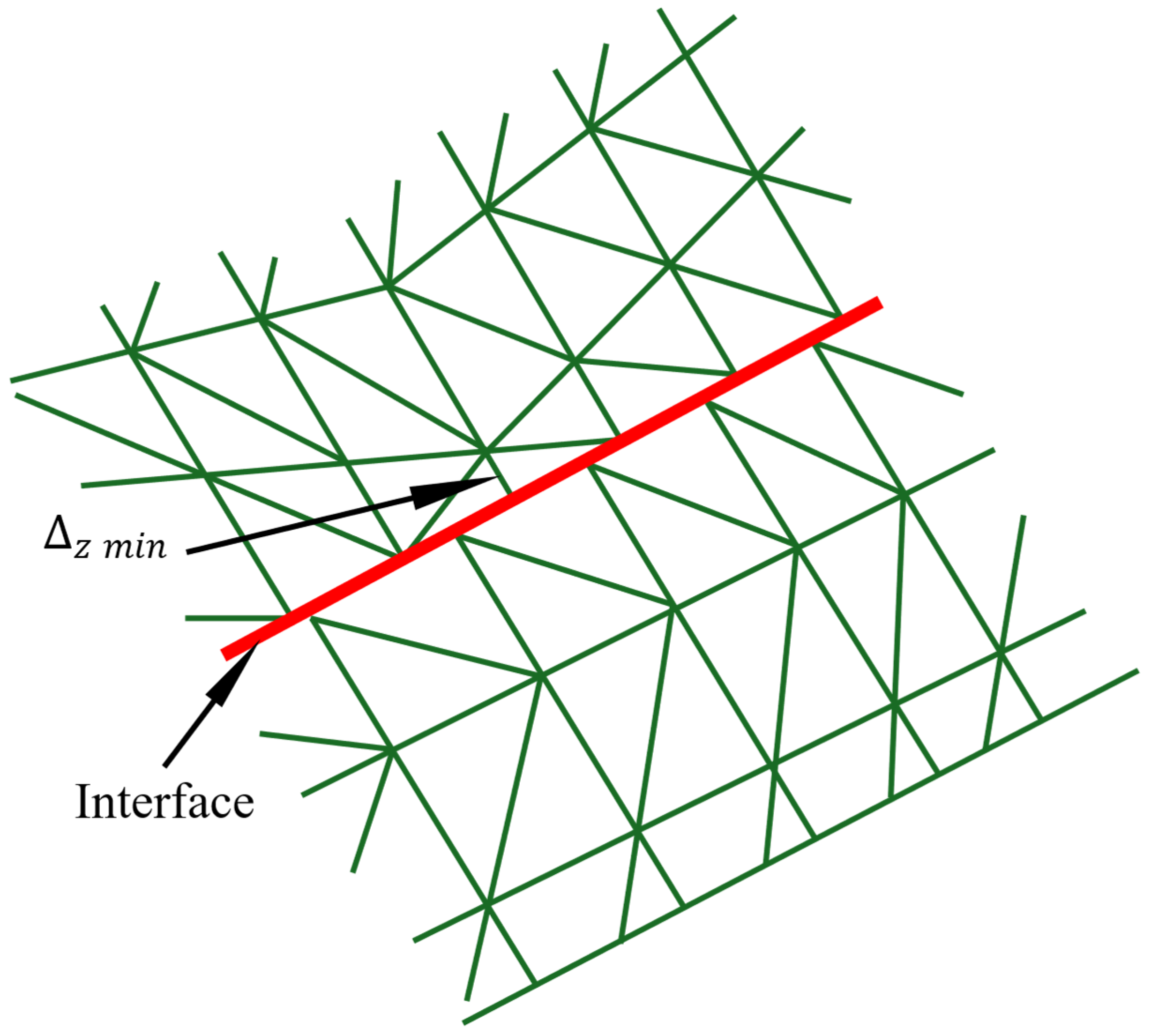
where $K$ and $G$ are bulk and shear moduli, respectively, of the block material, and ${∆z}_{min}$ is the smallest width of the zone adjoining the joint in the normal direction (Figure 7). If the joint stiffness values exceed 10 times the equivalent stiffness, the numerical solution time increases significantly without producing meaningful changes in the overall mechanical response of the model.

The stability of the critical block is assessed using the shear strength-to-shear stress ratio along the potential failure plane. UDEC allows this ratio to be monitored and plotted for the numerical zones adjacent to the joints within deformable blocks [22]. The parameter represents the ratio between the mobilized shear stress and the available shear strength along the discontinuity. Values approaching unity indicate that the shear strength of the joint is fully mobilized, corresponding to a factor of safety (FoS) approaching one and implying a limiting stability condition. In this study, the FoS is calculated under horizontal seismic loading by monitoring the shear strength-to-shear stress ratio during dynamic simulations.

Table 2. Input parameters used in the numerical simulations employing the C-Y joint model, including field-derived joint roughness parameters.

Intact Rock					Joint Properties
$\mathit{\gamma }$	$\mathit{E}$	$\mathit{\mu }$	${\mathit{\sigma }}_{\mathit{c}}\left(\mathit{J}\mathit{C}\mathit{S}\right)$	${\mathit{\sigma }}_{\mathit{t}}$	Joint	${\mathit{J}\mathit{R}\mathit{C}}_0$	${\mathit{J}\mathit{R}\mathit{C}}_{\mathit{r}}$	${\mathit{K}}_{\mathit{n}}$	${\mathit{K}}_{\mathit{s}}$	${\mathit{\varphi }}_{\mathit{j}}$
0.027	35	0.30	60	6.0	Joint Set 1	10.85	7.53	1.013	0.577	53
					Joint Set 2	7.35	5.21	1.438	0.693	46

Where $\gamma$ is the unit weight of intact rock (MN/m³), $E$ is the Young’s modulus (GPa), $\mu$ is the Poisson ratio, ${\sigma }_c$ is the joint compressive strength (MPa), ${\sigma }_t$ is the tensile strength (MPa), $K_n$ is the joint normal stiffness (GPa/m), $K_s$ is the shear stiffness (GPa/m), ${JRC}_0$ and ${JRC}_r$ are the initial and residual joint roughness coefficient, and ${\varphi }_j$ is the joint friction angle (degrees).

summarizes the input parameters used in the numerical simulations employing the continuous yielding (C-Y) joint model in UDEC. The initial joint roughness coefficient (${JRC}_0$) is derived from field mapping of discontinuities. To account for asperity degradation under cyclic shear induced by seismic loading, the residual joint roughness (${JRC}_r)$ is assumed to be 30% lower than the initial value, following recommendations from previous studies [28,32,33].

3.5. Model Geometry, Boundary Conditions, and Damping

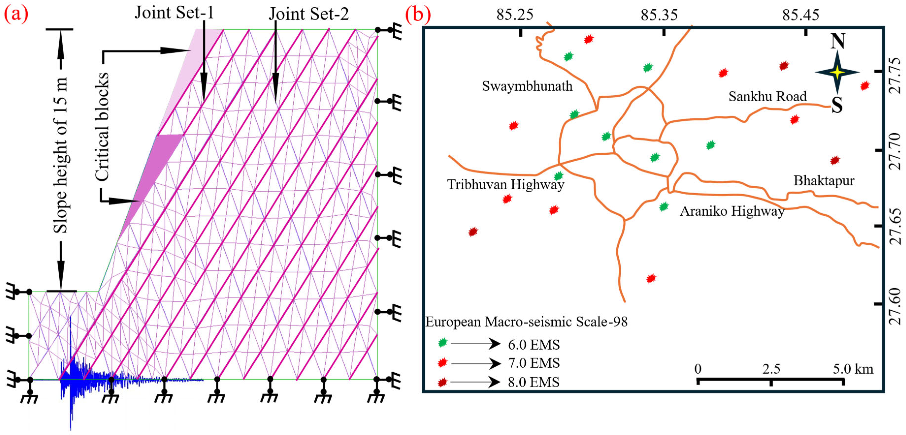
The numerical model geometry is constructed to represent the cross-sectional profile of the investigated rock-cut slope. Figure 8a shows the rock-slope profile that includes the slope height, inclination, and bench configuration. This profile is incorporated into the numerical model to replicate the actual geometric conditions of the site.

The discontinuity network is defined using dominant joint sets identified from the field mapping. The mean dip and dip-direction of the mapped joint sets are used to represent the orientation of discontinuities within the numerical model. These dominant joint sets are explicitly included in the numerical domain to simulate the behavior of the rock slope in jointed rock mass. The spacing of joints is assigned based on field mapping, allowing the model to capture the key structural features influencing slope stability. This enables realistic simulation of critical block movements and failure mechanisms governed by the interaction between slope face geometry and discontinuity sets.

The boundary conditions of the numerical model are defined to realistically simulate the dynamic response of the rock slope under dynamic loading. The lateral boundaries of the model are constrained in horizontal directions to prevent rigid body motion, while the base boundary is fixed in the vertical direction. To minimize artificial reflection of seismic waves at the model boundaries during dynamic analysis, viscous (quiet) boundary conditions are adopted along the lateral and bottom boundaries.

Rayleigh damping is employed to simulate energy dissipation during seismic loading, as it provides frequency-dependent damping that can be tuned to the dominant vibration modes of the slope [36]. A target damping ratio of 5% is selected, consistent with established practice for jointed rock mass [14,22].

3.6. Seismic Input Motions and Scaling

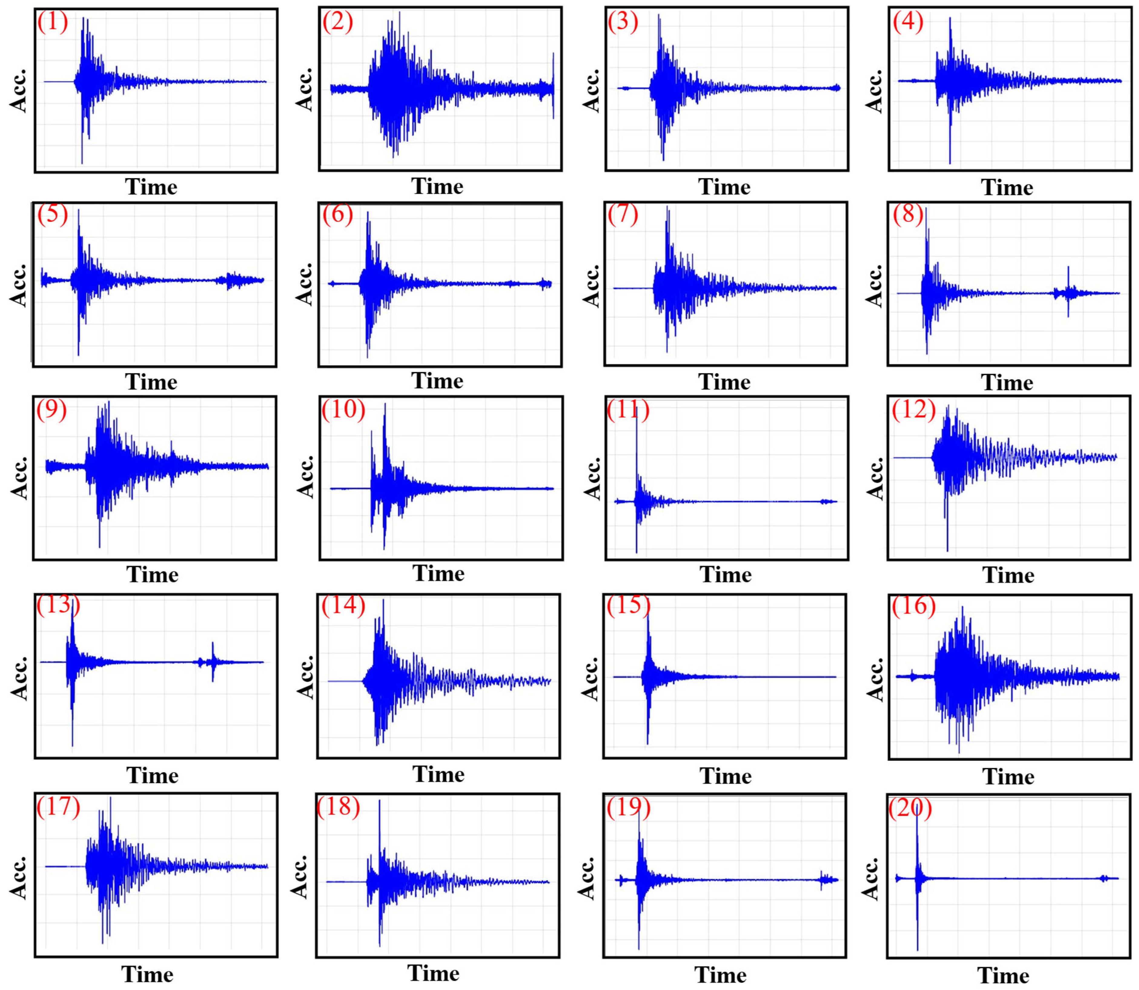
The seismic response of the jointed rock slope is evaluated using recorded ground motions applied as dynamic boundary conditions at the base of the numerical model. PGA is selected as the intensity measure for this study. PGA is widely used in rock-slope engineering practice and is easily understood by the designers. Twenty ground-motion records are selected, and their acceleration time histories are presented in Figure 9. The ground-motion records are selected from the 2015 Gorkha earthquake (Mw 7.8) recorded at different stations. The source-to-site distances range from approximately 80–120 km, representing far-field ground motions. The records are selected because the study area is located near the Main Boundary Thrust (MBT) and the epicenter of the Gorkha earthquake.

The original ground-motion records are provided as acceleration time histories (${\mathrm{m}/\mathrm{s}}^2$) sampled at discrete time intervals. However, UDEC’s dynamic solver requires velocity time histories as input boundary conditions [22]. Accordingly, acceleration records are converted to velocity time histories using numerical integration with baseline correction following Pacific Earthquake Engineering Research Center (PEER) ground-motion processing guidelines [37].

The trapezoidal rule is employed for integration, which provides second-order accuracy for uniformly sampled time-series data [9,36,38]:

$$v_i=v_{i-1}+{\displaystyle \frac{1}{2}}(a_{i-1}+a_i)∆t$$

(6)

where $v_i$ is the velocity at time step $i$, $∆t$ is the uniform sampling interval, and $v_0$ is the initial velocity (assumed to be zero). Baseline correction is applied to ensure zero net displacement at the end of each record, preventing artificial drift in the numerical model [39].

The velocity time histories are truncated to 20 s, as preliminary analysis indicates that the critical displacement response for most of the records occurs within this duration. This period captures the strong-motion phase of all records while maintaining computational efficiency in the simulations. Input files for each scaled velocity time history are prepared prior to dynamic analysis.

The UDEC model is first brought to static equilibrium under gravity loading (unbalanced force ratio $<{10}^{-5} \mathrm{M}\mathrm{N}$). Dynamic boundary conditions are then activated, and velocity histories are applied at the base of the model for 20 s. This two-stage procedure (static initialization followed by dynamic loading) ensures an accurate representation of slope response under seismic events.

3.7. Incremental Dynamic Analysis (IDA) Procedure

Incremental dynamic analysis (IDA) is performed to quantify the seismic response of the rock slope in jointed rock mass under progressively increasing earthquake intensities [10]. A set of recorded ground motions is applied as velocity time histories at the base of the model and systematically scaled to ten peak ground acceleration (PGA) levels ranging from 0.1 g to 1.0 g, which yielded 200 dynamic simulations.

To capture the non-linear dynamic shear behavior of rock joints, the continuously yielding (C-Y) joint model available in UDEC is adopted [22]. The C-Y model simulates progressive shear response along discontinuities following the B–B shear criterion. The effect of JRC mobilization during pre-peak and post-peak shear behavior is modeled following the degradation framework proposed by Asadollahi and Tonon [40] and Zhao [41]. The JRC degradation rate is calibrated from direct shear test data by Indraratna and Thirukumaran [42] and Oh and Cording [43]. This constitutive implementation allows for stress-dependent joint stiffness degradation, asperity damage, and dilation during cyclic seismic loading, which is consistent with observed behavior of rock joints under dynamic conditions [44].

For each scaled ground motion, an engineering demand parameter (EDP), defined as the residual displacement of the kinematically identified critical block at the end of the 20-s simulation, is recorded. IDA curves are constructed by plotting EDP against the corresponding intensity measure (IM), expressed as peak ground acceleration (PGA). The probabilistic seismic demand model (PSDM) is developed by fitting a log-linear regression to the ensemble of 200 EDP results [10,12]:

$$\ln \left(EDP\right)=a+bln\left(IM\right)$$

(7)

where $a$ and $b$ are regression coefficients obtained from least-squares fitting. The logarithmic standard deviation of demand (${\beta }_{EDP}$), also known as dispersion, is calculated using Equation (8).

$${\beta }_{EDP}=\sqrt{{\displaystyle \frac{{\displaystyle {\sum }_{i=1}^N}{\left[\ln \left({EDP}_i\right)-(a+b\ln \left({IM}_i\right))\right]}^2}{N-2}}}$$

(8)

where $N=200$ is the total number of IDA simulations, and ($N-2$) accounts for the two estimated regression parameters ($a \mathrm{a}\mathrm{n}\mathrm{d} b$).

The total dispersion is calculated by considering capacity uncertainty (${\beta }_C=0.3$) [45] and modeling uncertainty (${\beta }_M=0.4$), as suggested by Wen and Ellingwood [8] and Remo and Pinter [46]. Equation (9) represents the total log-normal dispersion parameter. This approach enables estimation of the median intensity (${IM}_{50}$) corresponding to 50% probability of exceedance for each damage state:

$${\beta }_{tot}=\sqrt{{\beta }_C^2+{\beta }_M^2+{\beta }_{EDP}^2}$$

(9)

3.8. Generation of Seismic Fragility Curve

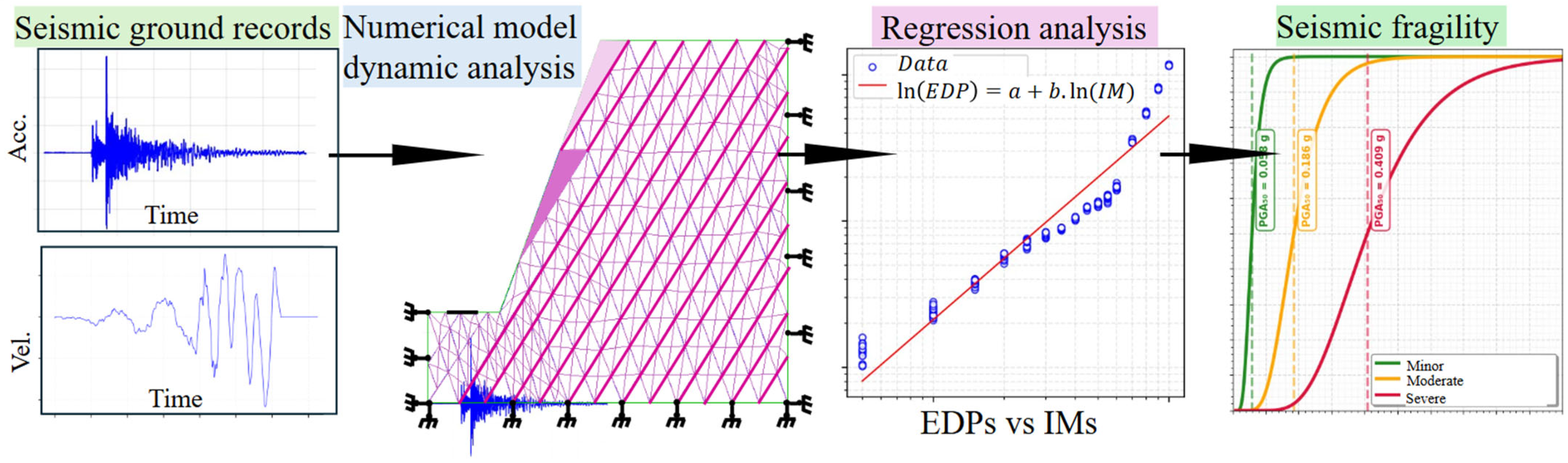
The seismic fragility curve is derived to quantify the probability that the seismic demand of the rock slope in jointed rock mass exceeds predefined damage states with increasing ground-motion intensity. Fragility analysis provides a probabilistic framework to evaluate the likelihood of slope damage or failure by combining the probabilistic seismic demand model (PSDM) with specified performance thresholds. Damage states are defined in terms of critical values of the selected engineering demand parameters (EDPs), such as maximum crest displacement and joint slip obtained from the dynamic numerical simulations. Figure 10 shows the methodological framework for seismic fragility curve development.

For each damage state, ${DS}_i$, the probability of exceedance is calculated assuming that the seismic demand follows a log-normal distribution conditioned on the IM. Equation (10) describes the seismic fragility curve that provides the conditional probability of being in or exceeding a particular damage state (${DS}_i$) for the given IM:

$$P_f\left[DS\ge {DS}_i⎸IM\right]=\mathit{\Phi }\left[{\displaystyle \frac{1}{{\beta }_{tot}}}\mathrm{l}\mathrm{n}\left({\displaystyle \frac{IM}{{IM}_{mi}}}\right)\right]$$

(10)

where $P_f$ represents the probability that a particular damage state, $DS$, is exceeded under a given level of seismic intensity. The seismic intensity level is represented by the peak ground acceleration (PGA) of the earthquake time histories. $\Phi \left[\dots \right]$ denotes the cumulative probability function, whereas ${IM}_{mi}$ represents the median threshold value of the earthquake intensity measure, which causes the damage associated with the ith state.

4. Results and Discussion

4.1. Dynamic Response of the Slope Under Earthquake Loading

Kinematic analysis is carried out using stereographic projection in Dips (Rocscience) to evaluate the feasibility of structurally controlled failure modes. The analysis indicates that planar failure is possible along joint set 1 with respect to the rock-slope face. Similarly, the intersection of joint set 1 and joint set 2 forms a potential line of intersection that may result in wedge failure.

To quantify the likelihood of these failure mechanisms considering the variability in discontinuity orientations, probabilistic kinematic analysis is performed using Monte Carlo simulation. The results indicate that the planar failure mechanism is dominant for this section of rock slope, with a probability of planar failure of approximately 90% (Figure 4a). Wedge failure is also possible, with an estimated probability of occurrence of about 52% (Figure 4b). Thus, the high probability of planar sliding along joint set 1 indicates that the geometric relationship between the discontinuity orientation and the slope face satisfies the kinematic daylighting condition. Under seismic loading, shear resistance along this joint set is progressively mobilized according to the non-linear B–B criterion, leading to cumulative slip along the potential failure plane.

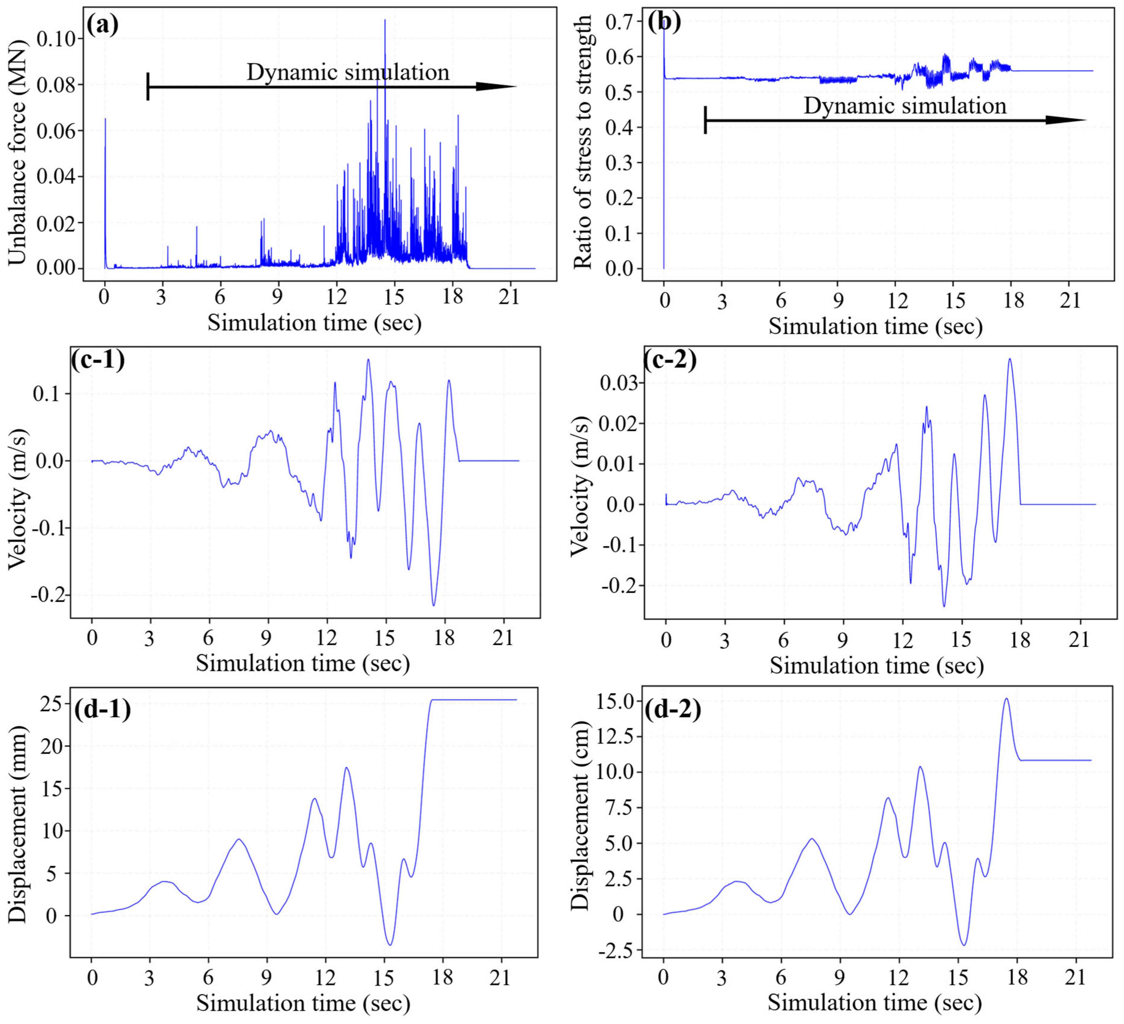
The dynamic input motions are applied at the base of the model (Figure 8a), and the resulting displacement of the critical block is monitored throughout the analysis. The simulations indicate that seismic loading induces progressive deformation within the rock mass along the slope, which is controlled by the orientation and the engineering geological properties of the discontinuities. The non-linear responses of the discontinuities are simulated using the C-Y joint model implemented in UDEC (Figure 11). The non-linear increase in residual displacement with increasing ground-motion intensity reflects the progressive mobilization of shear resistance along the discontinuity surfaces. At lower intensity levels, the joint asperities provide mechanical interlocking that limits relative movement. However, as seismic loading increases, shear stress exceeds the peak strength, resulting in progressive asperity degradation and cumulative slip along the critical joint surfaces. The dynamic response results obtained from the simulations provide the basis for the subsequent incremental dynamic analysis and probabilistic fragility assessment [12,13].

4.2. Incremental Dynamic Analysis Results and IM–EDP Relationship

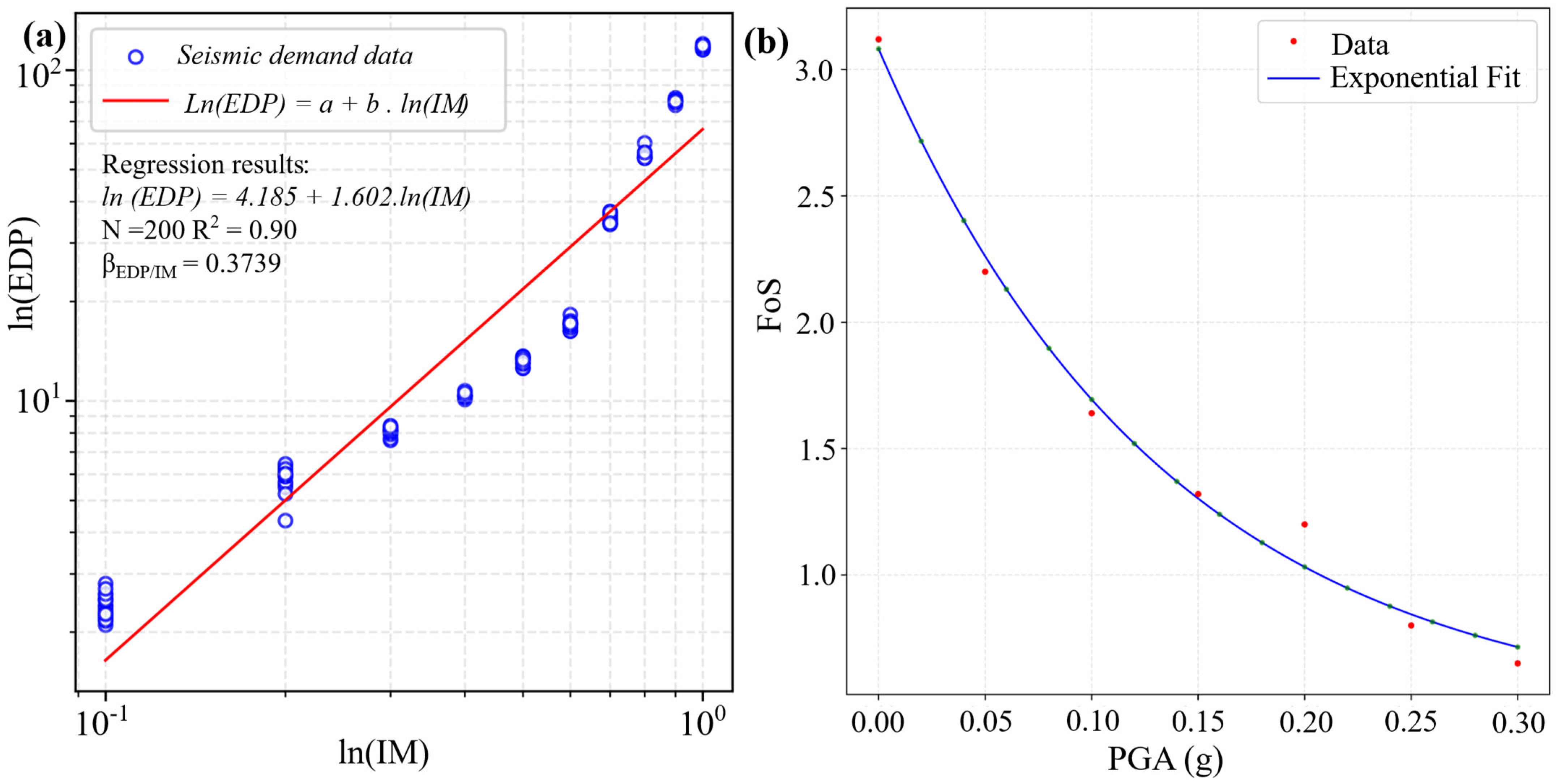
The incremental dynamic analysis (IDA) results illustrate the progressive seismic response of the jointed rock slope under increasing earthquake intensity levels. Figure 12a shows the relationship between the engineering demand parameter (EDP)–residual permanent displacement of the kinematically identified critical block– and the intensity measure (IM), expressed as peak ground acceleration (PGA).

The relationship between IM and EDP is quantified using log-linear regression applied to the ensemble of 200 IDA results. Regression analysis yielded coefficients $a=4.185$ and $b=1.602$, with a coefficient of determination $R^2=0.90$, indicating a good fit between the model and dataset (Figure 12a). The regression coefficient obtained indicates a strong dependency of displacement demand on ground-motion intensity. This suggests that once the seismic loading exceeds a certain threshold, the slope response becomes increasingly non-linear due to progressive joint slip and reduced shear resistance.

The logarithmic standard deviation of demand (${\beta }_{EDP}$), representing record-to-record variability, is calculated from regression using Equation (8), where $N=200$ and $N-2$ accounts for the two estimated regression parameters. This dispersion value is within the typical range for rock slopes (0.25–0.40) as reported by Salamon and Hariri-Ardebili [47].

In addition to displacement-based EDPs, the factor of safety (FoS) along the critical failure plane is computed using the shear strength-to-stress ratio approach in UDEC. The FoS exhibits exponential decay with increasing PGA (Figure 12b), providing an independent indicator of seismic slope performance. However, permanent displacement is selected as the primary EDP for fragility curve development.

4.3. Seismic Fragility Curves

Seismic fragility curves are developed to probabilistically evaluate the likelihood of the rock-slope failure exceeding predefined damage states under different levels of ground-motion intensity. Three displacement-based damage states are defined based on the residual permanent displacement of the critical block at the slope (Table 3 and Table 4).

Using a log-normal distribution framework, commonly adopted in performance-based earthquake engineering [13,48], the conditional probability of exceeding a displacement threshold ${(DS}_i)$ given as intensity measure ($IM$) is calculated using Equation (10). The regression coefficients from the probabilistic seismic demand model are $a=4.185$ and $b=1.602$ (Figure 12a).

Table 3. Seismic performance levels of slope in terms of permanent residual displacement [49].

Damage States	Slope Response	Permanent Residual Displacement (cm)
Intact	No risk	0$~$1
Partial damage	Local instability	1$~5$
Serious damage	Many local instabilities, risk	5$~15$
Overall instability	Sever collapse	$>15$

Table 3. Seismic performance levels of slope in terms of permanent residual displacement [49].

Damage States	Slope Response	Permanent Residual Displacement (cm)
Intact	No risk	0$~$1
Partial damage	Local instability	1$~5$
Serious damage	Many local instabilities, risk	5$~15$
Overall instability	Sever collapse	$>15$

Table 4. Seismic states of slopes in terms of factor of safety (FoS) [11].

Vulnerable States	Safety Margins	EDP Threshold
Unacceptable	None	$FoS<1$
Minor	Low	$1.0<FoS<1.25$
Moderate	Moderate	$1.25<FoS<1.4$
Sufficient	High	$FoS>1.4$

Table 4. Seismic states of slopes in terms of factor of safety (FoS) [11].

Vulnerable States	Safety Margins	EDP Threshold
Unacceptable	None	$FoS<1$
Minor	Low	$1.0<FoS<1.25$
Moderate	Moderate	$1.25<FoS<1.4$
Sufficient	High	$FoS>1.4$

The parameter ${\beta }_{tot}$ (Equation (9)) represents the total logarithmic standard deviation, which quantifies the combined effect of inherent variability and knowledge-based uncertainties. In this study, ${\beta }_{EDP}=0.3739$ is calculated from regression analysis, ${\beta }_C=0.30$ represents capacity uncertainty associated with threshold definition variability, and ${\beta }_M=0.40$ accounts for modeling uncertainty arising from numerical simplifications and constitutive assumptions. Substituting all these values yields ${\beta }_{tot}=0.62$.

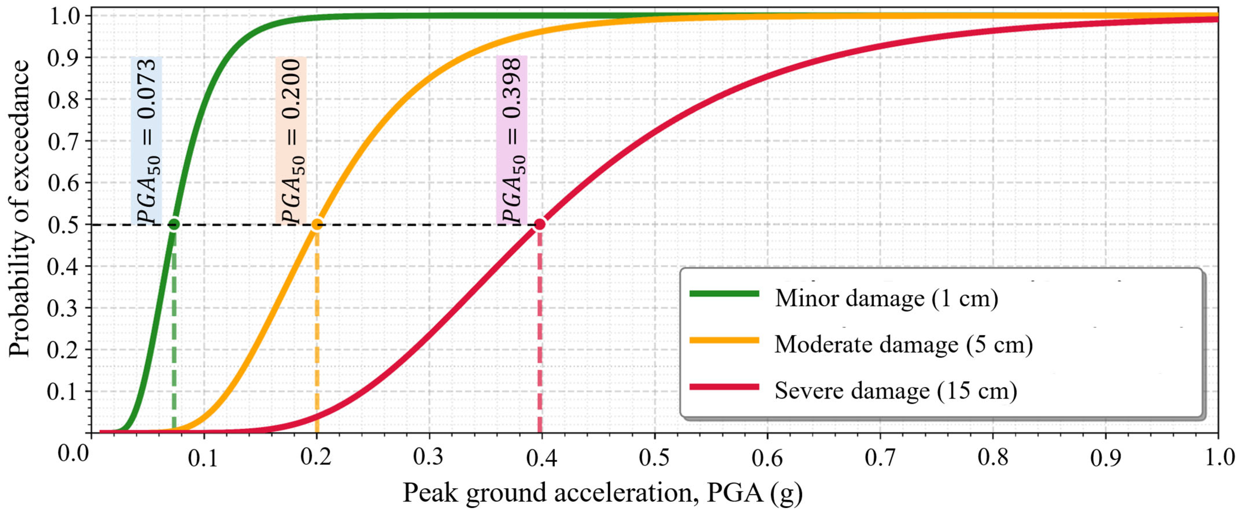
Seismic fragility curves are constructed by evaluating the probability equation over a continuous range of PGA values from 0.1 g to 1.0 g. Figure 13 represents the seismic fragility curves for the analyzed rock slope in jointed rock mass corresponding to three displacement-based damage states: minor (1 cm), moderate (5 cm), and severe (15 cm). The curves illustrate the probability of exceeding each damage state as a function of peak ground acceleration (PGA).

The median intensities corresponding to a 50% probability of exceedance are approximately 0.077 g for minor damage, 0.20 g for moderate damage, and 0.398 g for severe damage, indicating a progressive increase in the seismic demand required to trigger larger permanent displacements. The relatively low PGA₅₀ value for minor damage suggests that small joint opening and initial sliding may occur even under moderate seismic motion. In contrast, moderate and severe damage states require significantly higher ground-motion intensities, reflecting the additional shear resistance mobilized along the critical failure surfaces.

The wider spacing of the fragility curves also indicates increasing uncertainty in the displacement response at higher deformation levels. The steepness of the curves reflects the strong sensitivity of permanent displacement to increasing seismic intensity, which is consistent with the super-linear scaling relationship obtained. This behavior is attributed to the progressive degradation of joint shear strength captured by the Barton–Bandis criterion implemented through the continuously yielding (C-Y) joint model in the UDEC simulations. This formulation allows the model to capture asperity damage and dilation effects during cyclic loading, which contribute to the non-linear increase in permanent displacement with increasing ground-motion intensity.

4.4. Implications for Seismic Stability of Jointed Rock Slopes

The incremental dynamic analysis and derived fragility curves demonstrate that the slope exhibits a non-linear, deformation-dependent response under increasing earthquake intensity, emphasizing the importance of considering progressive yielding of discontinuities in seismic hazard assessment. The high probability of exceedance for moderate and severe damage indicates that the slope is highly sensitive to seismic loading.

The non-linear increase in displacement with PGA is explained by three stages of progressive joint degradation. Below 0.2 g, the joint behaves elastically with asperities intact. Between 0.2 g and 0.4 g, the JRC degrades. It is emphasized here that when the joint enters post-peak softening, even a small increase in PGA causes a large displacement. Therefore, it is logical that severe damage occurs at PGA as low as 0.4 g. The dominance of planar failure along joint set 1 (~90%) is controlled by joint orientation. The dip of joint set 1 is lower than the slope face, allowing the joint to daylight on the slope face. Under seismic loading, horizontal ground motion directly increases the driving force along the joint surface that is going to fail.

The fragility curves present three key features. First, the low PGA₅₀ for minor damage (0.077 g) indicates the slope is already near limit equilibrium under static conditions. The slope of a fragility curve indicates the degree of uncertainty. A flatter curve corresponds to higher uncertainty, meaning the damage state is exceeded over a wide PGA range. This reflects the complex and variable nature of progressive joint degradation and cumulative slip under different ground-motion conditions. As demonstrated by Hu et al. [11], fragility functions provide a more comprehensive and richer assessment of slope performance compared to deterministic approaches.

The findings highlight the necessity of integrating detailed field characterization with probabilistic numerical modeling for reliable seismic vulnerability assessment. Overall, structurally controlled rock slopes in tectonically active regions cannot be reliably assessed using deterministic approaches alone. Therefore, probabilistic methods are essential to capture inherent variability in joint orientations, material properties, and seismic motions.

5. Conclusions

This study has investigated the seismic stability and fragility of a rock slope of the jointed rock mass by integrating field characterization, probabilistic analysis, and dynamic numerical modeling. Based on the results obtained from structural mapping, incremental dynamic analysis, and fragility assessment, the following conclusions are drawn:

• Structural control of rock-slope stability: Field mapping identified two dominant joint sets in the rock mass controlling the structural behavior of the rock-slope. Kinematic analysis indicates that planar failure along joint set 1 represents the primary potential failure mechanism, while wedge failure formed by the intersection of joint set 1 and joint set 2 is also kinematically feasible.
• Probabilistic kinematic analysis: Monte Carlo simulation considering the statistical variability of discontinuity orientations indicates a high probability of planar failure (~90%) along joint set 1. Wedge failure associated with the intersection of joint set 1 and joint set 2 shows a lower but still significant probability (~52%), highlighting the influence of discontinuity geometry on this rock-slope.
• Dynamic response of the slope: Numerical simulations using the distinct element method in UDEC demonstrate that seismic loading induces progressive deformation concentrated along the mapped joint sets. The non-linear shear behavior of discontinuities modeled using the continuously yielding (C-Y) joint model leads to progressive mobilization of shear displacement and block movement during strong ground motion.
• Incremental dynamic analysis: IDA results show a non-linear increase in engineering demand parameters (EDPs). Significant deformation occurs once the seismic intensity exceeds moderate levels, indicating the sensitivity of structurally controlled rock-slope failure potential at earthquake loading.
• Seismic fragility assessment: Fragility curves derived from the probabilistic seismic demand model have demonstrated that the likelihood of slope damage increases rapidly with increasing seismic intensity.

Overall, the analysis results have demonstrated that the seismic stability of rock slopes in jointed rock mass is strongly governed by discontinuity geometry and non-linear joint behavior. The integration of field-based joint characterization, probabilistic kinematic analysis, and dynamic numerical modeling provides a robust framework for evaluating the seismic vulnerability of structurally controlled rock slopes. The authors are convinced that the proposed approach may support more reliable hazard assessment and the design of mitigation measures for rock slopes in seismically active regions.

6. Limitations and Future Work

Despite the comprehensive methodology adopted in this study, several limitations should be acknowledged. The limited number of field observation data may not fully represent the spatial variability of the rock mass. Increasing the number of field observations would improve the statistical reliability of the discontinuity orientation data.

In addition, the engineering geological properties of joints, particularly the joint roughness coefficient (JRC) and joint compressive strength (JCS), are estimated from field observations, mapping, measurement, and empirical correlations. Since JRC and JCS are critical parameters that control the non-linear shear behavior of discontinuities in the B–B model, the use of calibrated parameters obtained from in situ direct shear tests would provide more realistic estimates of joint shear strength. However, such in situ shear tests are not conducted in the present study, which represents an important limitation.

Furthermore, the numerical simulations are performed using a two-dimensional distinct element model, which may not fully capture three-dimensional block interactions and complex failure geometries. Future studies should therefore consider larger field datasets, in situ shear testing for calibration of joint parameters, and three-dimensional numerical modeling to improve the reliability of seismic fragility assessment of jointed rock slopes.

References

1. Panthi, K.K. Assessment on the 2014 Jure Landslide in Nepal—A Disaster of Extreme Tragedy. In Proceedings of the ISRM International Symposium–EUROCK 2021, Virtual, 21–24 September 2021. [Google Scholar]
2. Ahmed, I.; Shang, Y.; Sousa, L.; Meng, Q.; Tanoli, J.I.; Waqar, M.F. Geomechanical evaluation of fault damage zone in the active Himalayas of Northern Pakistan. Environ. Earth Sci. 2025, 84, 644. [Google Scholar] [CrossRef]
3. Dubey, S.; Sattar, A.; Goyal, M.K.; Allen, S.; Frey, H.; Haritashya, U.K.; Huggel, C. Mass movement hazard and exposure in the Himalaya. Earth’s Future 2023, 11, e2022EF003253. [Google Scholar] [CrossRef]
4. Wang, W.; Li, D.-Q.; Tang, X.-S.; Du, W. Seismic fragility and demand hazard analyses for earth slopes incorporating soil property variability. Soil Dyn. Earthq. Eng. 2023, 173, 108088. [Google Scholar] [CrossRef]
5. Hoek, E.; Bray, J.D. Rock Slope Engineering; CRC Press: Boca Raton, FL, USA, 1981. [Google Scholar]
6. Xu, C.; Liu, Q.; Tang, X.; Sun, L.; Deng, P.; Liu, H. Dynamic stability analysis of jointed rock slopes using the combined finite-discrete element method (FDEM). Comput. Geotech. 2023, 160, 105556. [Google Scholar] [CrossRef]
7. Hu, C.; Lei, R.; Berto, F. System Reliability Assessment of Rock Slopes Under Seismic Loading Considering the Spatial Variability of Strength Parameters. Rock Mech. Rock Eng. 2025, 58, 9297–9310. [Google Scholar] [CrossRef]
8. Wen, Y.; Ellingwood, B.; Veneziano, D.; Bracci, J. Uncertainty Modeling in Earthquake Engineering; MAE Center Project FD-2 Report; Mid-America Earthquake Center, University of Illinois at Urbana-Champaign: Champaign, IL, USA, 2003. [Google Scholar]
9. Kramer, S.L. Geotechnical Earthquake Engineering; Prentice hall: New York, NY, USA, 1996; 794p. [Google Scholar]
10. Vamvatsikos, D.; Cornell, C.A. Incremental dynamic analysis. Earthq. Eng. Struct. Dyn. 2002, 31, 491–514. [Google Scholar] [CrossRef]
11. Hu, H.; Huang, Y.; Chen, Z. Seismic fragility functions for slope stability analysis with multiple vulnerability states. Environ. Earth Sci. 2019, 78, 690. [Google Scholar] [CrossRef]
12. Jalayer, F.; Cornell, C.A. Alternative non-linear demand estimation methods for probability-based seismic assessments. Earthq. Eng. Struct. Dyn. 2009, 38, 951–972. [Google Scholar] [CrossRef]
13. Cornell, C.A.; Jalayer, F.; Hamburger, R.O.; Foutch, D.A. Probabilistic basis for 2000 SAC federal emergency management agency steel moment frame guidelines. J. Struct. Eng. 2002, 128, 526–533. [Google Scholar] [CrossRef]
14. Hariri-Ardebili, M.; Saouma, V. Collapse fragility curves for concrete dams: Comprehensive study. J. Struct. Eng. 2016, 142, 04016075. [Google Scholar] [CrossRef]
15. Barton, N.; Bandis, S. Effects of block size on the shear behavior of jointed rock. In Proceedings of the ARMA US Rock Mechanics/Geomechanics Symposium, Berkeley, CA, USA, 25–27 August 1982; American Institute of Mining, Metallurgical, and Petroleum Engineers: New York, NY, USA, 1982; pp. 739–760. [Google Scholar]
16. Bandis, S.; Lumsden, A.; Barton, N. Fundamentals of rock joint deformation. Int. J. Rock Mech. Min. Sci. Geomech. Abstr. 1983, 20, 249–268. [Google Scholar] [CrossRef]
17. Tatone, B.S.; Grasselli, G. An investigation of discontinuity roughness scale dependency using high-resolution surface measurements. Rock Mech. Rock Eng. 2013, 46, 657–681. [Google Scholar] [CrossRef]
18. Bommer, J.J.; Acevedo, A.B. The use of real earthquake accelerograms as input to dynamic analysis. J. Earthq. Eng. 2004, 8, 43–91. [Google Scholar] [CrossRef]
19. Liu, X.; Wang, Y. Probabilistic hazard analysis of rainfall-induced landslides at a specific slope considering rainfall uncertainty and soil spatial variability. Comput. Geotech. 2023, 162, 105706. [Google Scholar] [CrossRef]
20. Sotiriadis, D.; Klimis, N.; Koutsoupaki, E.I.; Petala, E.; Valkaniotis, S.; Taftsoglou, M.; Margaris, V.; Dokas, I. Toward a plausible methodology to assess rock slope instabilities at a regional scale. Geosciences 2023, 13, 98. [Google Scholar] [CrossRef]
21. Katsanos, E.I.; Sextos, A.G.; Manolis, G.D. Selection of earthquake ground motion records: A state-of-the-art review from a structural engineering perspective. Soil Dyn. Earthq. Eng. 2010, 30, 157–169. [Google Scholar] [CrossRef]
22. Board, M. UDEC (Universal Distinct Element Code) Version ICG1. 5; Nuclear Regulatory Commission; Division of High-Level Waste Management, Office of Nuclear Material Safety and Safeguards, U.S. Nuclear Regulatory Commitions: Washington, DC, USA, 1989. [Google Scholar]
23. Dhital, M.R. Geology of the Nepal Himalaya: Regional Perspective of the Classic Collided Orogen; Springer: Berlin/Heidelberg, Germany, 2015. [Google Scholar]
24. Panthi, K.K. Analysis of Engineering Geological Uncertainties Related to Tunnelling in Himalayan Rock Mass Conditions. Ph.D. Thesis, Norges Teknisk-Naturvitenskapelige Universitet, Trondheim, Norway, 2006. [Google Scholar]
25. Upreti, B. An overview of the stratigraphy and tectonics of the Nepal Himalaya. J. Asian Earth Sci. 1999, 17, 577–606. [Google Scholar] [CrossRef]
26. Hoek, E.; Bray, J.; Boyd, J. The stability of a rock slope containing a wedge resting on two intersecting discontinuities. Q. J. Eng. Geol. Hydrogeol. 1973, 6, 1–55. [Google Scholar] [CrossRef]
27. Barton, N.; Choubey, V. The shear strength of rock joints in theory and practice. Rock Mech. 1977, 10, 1–54. [Google Scholar] [CrossRef]
28. Barton, N.; Wang, C.; Yong, R. Advances in joint roughness coefficient (JRC) and its engineering applications. J. Rock Mech. Geotech. Eng. 2023, 15, 3352–3379. [Google Scholar] [CrossRef]
29. Barton, N. Review of a new shear-strength criterion for rock joints. Eng. Geol. 1973, 7, 287–332. [Google Scholar] [CrossRef]
30. Jiang, Q.; Liu, X.; Wei, W.; Zhou, C. A new method for analyzing the stability of rock wedges. Int. J. Rock Mech. Min. Sci. 2013, 60, 413–422. [Google Scholar] [CrossRef]
31. Cundall, P.A. A computer model for simulating progressive, large-scale movements in blocky rock systems. In Proceedings of the ISRM International Symposium, Nancy, France, 4–6 October 1971. [Google Scholar]
32. Shen, J.; Tao, R.; Bao, X.; Chen, B.; Cui, H.; Chen, X. Study about influence of RC segment degradation on seismic response of shield tunnel. Case Stud. Constr. Mater. 2025, 22, e04615. [Google Scholar] [CrossRef]
33. Qi, S.; Zheng, B.; Guo, S.; Luo, G. A new shear strength criterion for rock discontinuities considering roughness degradation and loading rate effect. Int. J. Rock Mech. Min. Sci. 2025, 194, 106231. [Google Scholar] [CrossRef]
34. Martin, S.S.; Hough, S.E.; Hung, C. Ground motions from the 2015 M w 7.8 Gorkha, Nepal, earthquake constrained by a detailed assessment of macroseismic data. Seismol. Res. Lett. 2015, 86, 1524–1532. [Google Scholar] [CrossRef]
35. Yagi, Y.; Okuwaki, R. Integrated seismic source model of the 2015 Gorkha, Nepal, earthquake. Geophys. Res. Lett. 2015, 42, 6229–6235. [Google Scholar] [CrossRef]
36. Chopra, A.K. Dynamics of Structures; Pearson Education India: Chennai, India, 2007. [Google Scholar]
37. Baker, J.W.; Lin, T.; Shahi, S.K.; Jayaram, N. New ground motion selection procedures and selected motions for the PEER transportation research program. PEER Rep. 2011, 3, 2011. [Google Scholar]
38. Newmark, N.M. A method of computation for structural dynamics. J. Eng. Mech. Div. 1959, 85, 67–94. [Google Scholar] [CrossRef]
39. Boore, D.M.; Bommer, J.J. Processing of strong-motion accelerograms: Needs, options and consequences. Soil Dyn. Earthq. Eng. 2005, 25, 93–115. [Google Scholar] [CrossRef]
40. Asadollahi, P.; Tonon, F. Constitutive model for rock fractures: Revisiting Barton’s empirical model. Eng. Geol. 2010, 113, 11–32. [Google Scholar] [CrossRef]
41. Zhao, J. Joint surface matching and shear strength part A: Joint matching coefficient (JMC). Int. J. Rock Mech. Min. Sci. 1997, 34, 173–178. [Google Scholar] [CrossRef]
42. Indraratna, B.; Thirukumaran, S.; Brown, E.; Zhu, S.-P. Modelling the shear behaviour of rock joints with asperity damage under constant normal stiffness. Rock Mech. Rock Eng. 2015, 48, 179–195. [Google Scholar] [CrossRef]
43. Oh, J.; Cording, E.; Moon, T. A joint shear model incorporating small-scale and large-scale irregularities. Int. J. Rock Mech. Min. Sci. 2015, 76, 78–87. [Google Scholar] [CrossRef]
44. Cui, Z.; Sheng, Q.; Leng, X. Analysis of S wave propagation through a nonlinear joint with the continuously yielding model. Rock Mech. Rock Eng. 2017, 50, 113–123. [Google Scholar] [CrossRef]
45. Huang, Z.-K.; Pitilakis, K.; Tsinidis, G.; Argyroudis, S.; Zhang, D.-M. Seismic vulnerability of circular tunnels in soft soil deposits: The case of Shanghai metropolitan system. Tunn. Undergr. Space Technol. 2020, 98, 103341. [Google Scholar] [CrossRef]
46. Remo, J.W.; Pinter, N. Hazus-MH earthquake modeling in the central USA. Nat. Hazards 2012, 63, 1055–1081. [Google Scholar] [CrossRef]
47. Salamon, J.W.; Hariri-Ardebili, M.A. Verification, validation, and uncertainty quantification (VVUQ) in structural analysis of concrete dams. Front. Built Environ. 2024, 10, 1452415. [Google Scholar] [CrossRef]
48. Scawthorn, C.; Flores, P.; Blais, N.; Seligson, H.; Tate, E.; Chang, S.; Mifflin, E.; Thomas, W.; Murphy, J.; Jones, C. HAZUS-MH flood loss estimation methodology. II. Damage and loss assessment. Nat. Hazards Rev. 2006, 7, 72–81. [Google Scholar] [CrossRef]
49. Jibson, R.W. Methods for assessing the stability of slopes during earthquakes—A retrospective. Eng. Geol. 2011, 122, 43–50. [Google Scholar] [CrossRef]
Figure 1. Block diagram of the Nepal Himalaya showing various lithologies and major thrusts [24].
Geosciences 16 00203 g001
Figure 2. Geological maps of the study area: (a) illustration of lithology for rock formations; (b) peak ground acceleration contour map of Nepal (Department of Mines, Nepal).
Geosciences 16 00203 g002
Figure 3. (a) Photograph of the site taken while field mapping; (b) kinematic analysis is performed, showing the possibility of planar and wedge modes of failure.
Geosciences 16 00203 g003
Figure 4. Distribution of mode of probability failure: (a) planar failure probability along the joint Set 1; (b) wedge failure probability due to joint set 1 and joint set 2.
Geosciences 16 00203 g004
Figure 5. Statistical distribution of joint roughness coefficient (JRC) values derived from field mapping of dominant joint surfaces: (a) Joint Set 1 and (b) Joint Set 2. Histograms with fitted normal distribution curves illustrate the variability of JRC used in the subsequent shear strength analysis.
Geosciences 16 00203 g005
Figure 6. Geometry of biplane failure case, showing various planes and effective normal reaction forces acting on respective planes.
Geosciences 16 00203 g006
Figure 7. Schematic illustration of the minimum zone width ( z m i n ) in the normal direction to the joint used for calculating the equivalent stiffness of adjacent zones in the UDEC model.
Geosciences 16 00203 g007
Figure 8. (a) Numerical model geometry of the jointed rock slope showing slope profile, dominant joint sets, boundary conditions, unstable critical blocks, and applied seismic loading incorporated in the distinct element model; (b) location of recorded seismic time-history data are applied for the generation of fragility curves [34,35]. The recording stations are located approximately 120 km from the study area.
Geosciences 16 00203 g008
Figure 9. Acceleration time histories of 20 earthquake ground-motion records obtained from seismic stations located near the study area (Figure 8b). Twenty (1–20) acceleration time history records used in the analysis.
Geosciences 16 00203 g009
Figure 10. Workflow procedures for seismic fragility curve development of the jointed rock slope, including selection and scaling of seismic ground-motion records, dynamic numerical analysis to obtain engineering demand parameters (EDPs), regression analysis between EDPs and Intensity measures (IMs), and derivation of fragility curves for different damage states.
Geosciences 16 00203 g010
Figure 11. Dynamic response histories from the UDEC simulation: (a) unbalanced force history used to verify numerical equilibrium; (b) shear stress–strength ratio (FoS) along the critical failure plane based on the C-Y joint model; (c-1,c-2) representatives scaled input velocity histories applied at the model base; and (d-1,d-2) corresponding residual permanent displacement histories of the critical rock-slope block.
Geosciences 16 00203 g011
Figure 12. (a) Log-log regression relationship between residual permanent displacement of the critical block (EDP) and peak ground acceleration (PGA) used as the intensity measure (IM), showing the fitted model parameters a, b and R 2 ; (b) Variation of the factor of safety (FoS), derived from the shear stress-to-shear strength ratio along the potential sliding plane, with increasing PGA obtained from UDEC dynamic simulations.
Geosciences 16 00203 g012
Figure 13. Seismic fragility curves showing the probability of exceeding minor (1 cm), moderate (5 cm), and severe (15 cm) displacement damage states for the analyzed jointed rock slope as a function of peak ground acceleration (PGA). Vertical dashed lines indicate the median intensity ( P G A 50 ) corresponding to a 50% probability of exceedance.
Geosciences 16 00203 g013