Differences in Carbon Emissions and Spatial Spillover in Typical Urban Agglomerations in China

Abstract

This study investigates the spatial patterns and drivers of carbon emissions across China’s three major urban agglomerations—Beijing–Tianjin–Hebei (BTH), the Yangtze River Delta (YRD), and the Pearl River Delta (PRD)—from 2011 to 2020. A sequential analytical framework was employed to examine emission inequality, spatial dependence, dynamic transitions, and multi-scale drivers. Specifically, the Gini and Theil indices were used to quantify and decompose regional disparities. Spatial clustering patterns and heterogeneity were then identified through global and local Moran’s I analysis. Following this, spatial Markov chains modeled state transitions and neighborhood spillover effects. Finally, the Spatial Durbin Model (SDM) was applied to distinguish between the direct and indirect effects of key socioeconomic drivers. The findings reveal that disparities in emissions are largely driven by factors within each region. In BTH, heavy industrial lock-in accounts for 47.1% of the within-group inequality. By contrast, the YRD and PRD show noticeable convergence, achieved through industrial synergy and technological restructuring, respectively. The mechanisms of spatial spillover also differ across regions. In the YRD, emissions exhibit strong clustering tied to geographic proximity, with Moran’s I consistently above 0.6. In BTH, policy linkages play a more central role in shaping emission patterns. Meanwhile, in the PRD, widespread technological diffusion weakens the conventional distance-decay effect. The influence of key drivers varies notably among the urban agglomerations. Economic growth has the strongest scale effect in the PRD, reflected by a coefficient of 0.556. Industrial transformation significantly lowers emissions in the YRD, with a coefficient of −0.115. Technology investment reduces emissions in BTH (−0.124) and the PRD (−0.076), but is associated with a slight rebound in the YRD (0.037). Overall, these results highlight the persistent path dependence and distinct spatial interdependencies of carbon emissions in each region. This underscores the need for tailored mitigation strategies that are coordinated across administrative boundaries.

1. Introduction

Empirical evidence demonstrates that accelerated industrialization and anthropogenic greenhouse gas emissions have markedly amplified radiative forcing, thereby intensifying global surface warming and imposing pervasive pressures on human–environment systems [1]. In response, the Intergovernmental Panel on Climate Change (IPCC) advocates for rapid, large reductions in fossil-fuel-related CO₂ emissions to limit the global mean temperature rise to well below 2 °C above pre-industrial levels. This imperative has been codified in successive multilateral instruments, most notably the 1997 Kyoto Protocol and the 2015 Paris Agreement, which have established common but differentiated responsibilities for emission abatement [2]. Consequently, carbon mitigation has risen to prominence across public, private, and academic spheres worldwide. Since surpassing the United States in 2007, China has remained the world’s largest energy consumer and the single largest national source of anthropogenic CO₂. By 2016, its per capita emissions had nearly doubled relative to 2000, while national emissions accounted for roughly 30% of the global total [3]. Confronting the dual imperative of decarbonization and sustained economic growth, China has implemented an increasingly stringent portfolio of mitigation measures designed to achieve absolute emission reductions without compromising GDP growth [4]. In 2007, the National Development and Reform Commission (NDRC) released China’s National Climate Change Program, with the country committing to achieving zero or negative carbon-emission growth by mid-century. In late 2009, on the eve of COP15 in Copenhagen, China pledged to reduce the economy-wide carbon intensity—measured as CO₂ per unit GDP—by 40–45% below 2005 levels by 2020. On 22 September 2020, during the 75th United Nations General Assembly, China further elevated its ambition by announcing its intention to reach peak national CO₂ emissions before 2030 and to attain carbon neutrality by 2060 [5].

Urban agglomerations represent critical spatial units for climate mitigation, serving as both economic powerhouses and the primary sources of energy consumption and anthropogenic CO₂ emissions [6,7]. In China, BTH, the YRD, and the PRD exemplify this dual character. Together, they generated more than 34.8% of the national GDP in 2015, while also acting as core hubs of energy use and territorial carbon emissions [8]. As engines of economic growth and crucial leverage points for decarbonization, the low-carbon transition of these regions is essential for achieving China’s dual-carbon goals [9].

Significant heterogeneity in industrial structure, resource endowment, and developmental stages among constituent cities gives rise to substantial carbon leakage risks. These risks emerge through the spatial relocation of pollution-intensive activities, which exacerbates institutional and physical barriers to cross-jurisdictional sharing of low-carbon infrastructure. Addressing these challenges requires transcending fragmented administrative boundaries through regionally integrated strategies. Such strategies may include promoting industrial complementarity, developing interoperable transport networks, establishing reciprocal energy supply mechanisms, and advancing ecological co-governance. Collectively, these measures can achieve systemic emission reduction co-benefits that are beyond the reach of individual cities [10,11,12].

Furthermore, these agglomerations offer distinct advantages for policy piloting. They enable detailed disaggregation of emission drivers, harmonization of monitoring and accounting protocols, integration of carbon markets, and collaborative development of green finance instruments. The resulting evidence-based policy toolkits not only accelerate economy-wide decarbonization but also provide scalable governance models that can be extended nationwide [13].

Within urban agglomerations, divergent development stages and industrial specialization lead to significant heterogeneity in energy-related carbon emissions, with the timing of aggregate peak emissions being strongly influenced by economic maturity. The mature Northeast U.S. megaregion (per capita GDP ≈ USD 62,030) reached its carbon peak in 2007, while the Northwestern European Urban Agglomeration (per capita GDP ≈ USD 45,652) has maintained an annual decline of 1.8% since that year. The Japanese Pacific Coastal Urban Agglomeration (per capita GDP ≈ USD 48,315), still in a catch-up phase, underwent volatile plateau-like fluctuations and peaked in 2013 [14]. By contrast, the developing Mumbai Metropolitan Region (per capita GDP ≈ USD 8200) showed a steady upward trend, averaging an increase of 4.2% per annum [15].

High-income regions with urbanization rates exceeding 80% have transitioned territorial CO₂ emissions to a declining trajectory, whereas developing nations continue to experience emission growth, primarily driven by infrastructure expansion. For instance, urban infrastructure accounts for 42% of India’s final energy consumption. Industrial specialization and integration into global value chains further influence emission intensity. The Greater South East UK region illustrates a “smiling-curve” configuration: London’s high-value financial services and Birmingham’s intermediate manufacturing form low-carbon cores, which are surrounded by peripheries with moderately higher carbon emissions [14]. However, per capita residential energy consumption in affluent cores is still significantly higher than in peripheral cities [16]. Conversely, driven by a comprehensive shift in energy mix and strategic industrial clustering, Japan’s manufacturing sector significantly reduced its CO₂ emissions between 2008 and 2019. In contrast, horizontally specialized manufacturing clusters in Southeast Asia, which are marked by intense homogeneous competition, tend to produce higher carbon emissions throughout the entire value chain [17].

To meet their mitigation targets, developed regions frequently offset their carbon emissions by importing carbon-intensive goods from less developed regions, thereby displacing net emissions [18]. Industries such as steel, cement, and fossil-fuel derivatives, which are characterized by highly energy-intensive production processes, act as the principal conduits for the spatial transfer of embodied carbon [19,20]. For example, the embodied carbon emissions associated with China’s exports of steel and mechanical–electrical products to Europe and the United States account for more than 40% of the total embodied carbon in Chinese merchandise exports [21]. As a result, consumption-based carbon emissions in the United States, the European Union, and Japan are approximately 5% lower than their production-based emissions, whereas China’s consumption-based emissions are more than 15% higher, highlighting the asymmetry between net carbon importers and exporters [22].

Moreover, carbon transfers among emerging economies have become increasingly pronounced, with significant growth in carbon-intensive trade patterns. For instance, China’s semi-finished steel exports to Southeast Asia are processed there before being re-exported to Europe and North America, forming transnational carbon-transfer chains [23]. Similar mechanisms are observed within national and regional boundaries. For example, Beijing, Shanghai, and Tianjin transfer emissions to resource-rich provinces such as Hebei, Shanxi, and Inner Mongolia through domestic trade. Approximately 69% of Beijing’s consumption-based emissions are attributed to imports from Hebei and Shandong via interprovincial trade [24]

Improvements in transport infrastructure and rising productivity facilitate the inter-regional exchange of production inputs and the redistribution of value, leading to denser and more frequent embodied carbon transfers. As a result, aggregate emissions may remain stagnant, which undermines mitigation incentives and lowers abatement efficiency in less-developed regions [25]. By leveraging geographic and historical advantages, advanced cities can rapidly integrate into global value chains, accumulate capital and upgrade technologies, thereby significantly increasing economic output and restructuring their industrial composition. As energy-intensive industries formerly housed in developed economies lose competitiveness, they are often relocated to lagging regions [26]. Moreover, enhanced transport networks reduce the inhibiting effect of distance on trade, thereby facilitating carbon transfers, particularly within urban agglomerations [27,28].

Intra-regional carbon emission transfers typically exhibit spillover effects, which are primarily mediated by economic–technological linkages, industrial specialization, policy coordination, and spatial connectivity, thereby extending their impacts to adjacent or interconnected regions. Studies demonstrate that spatial spillovers decay with distance, with neighboring regions exhibiting pronounced spatial dependence in carbon emission efficiency or intensity due to industrial linkages and population mobility. For instance, Lü et al. [29] analyzed data from 98 countries and found that the spatial lag coefficients of per capita CO₂ emissions ranged from 0.21 to 0.45 (using geographic distance weighting) and from 0.13 to 0.32 (using economic distance weighting), indicating significant spatial dependence in carbon emissions. At the county level within the Harbin–Changchun Urban Agglomeration, carbon emissions exhibit a highly significant spatial correlation, with notable spatial spillovers in efficiency changes among neighboring cities [30].

Scholars employ diverse methodologies to assess regional spillovers of carbon emissions. For example, Dong [31] analyzed embodied carbon in bilateral trade between China and Japan using the Asian Input–Output Table. Meanwhile, Chen et al. [32] applied a land use transfer matrix and a modified Kaya-LMDI model, finding that the conversion of land to construction use in BTH is the primary driver of increased carbon emissions, with the spatial distribution of emissions showing a northeast–southwest agglomeration pattern. However, as multi-regional input–output (MRIO) models and spatial panel models may fail to capture complex spatial relationships, researchers increasingly adopt spatial Markov-chain methods. For instance, Wang et al. [33] applied the Gini index and spatial autocorrelation analysis to urban-level energy consumption and carbon emission data, revealing significant path dependence in the evolution of carbon emission patterns.

Building upon the existing literature, two primary research gaps can be identified. Theoretically, prior studies often inadequately capture how spatial context constrains and shapes the evolutionary pathways of urban carbon emissions, particularly in terms of multi-scale dependence and nonlinear spillover mechanisms. Methodologically, conventional approaches, such as standard spatial panel or input–output models, frequently struggle to disentangle the complex interactions between local factors and cross-boundary spillover effects, thus limiting the precision of policy-oriented analysis. To address these gaps, this study makes distinct theoretical and methodological contributions. Theoretically, it develops a multi-scale, multidimensional analytical framework that explicitly examines how spatial context—including neighborhood conditions and regional linkages—constrains and transmits carbon emission dynamics. Methodologically, it integrates spatial Markov chains to model state transitions under spatial dependence and employs a Spatial Durbin Model (SDM) to separately identify the direct effects of local drivers and the indirect spillover effects from neighboring areas. This approach enhances the empirical precision of identifying spatial spillovers and their policy implications.

In this context, this study selects three of the most developed urban agglomerations in China—BTH, the PRD and the YRD—as research subjects. We will first employ the Gini index and Theil index to analyze the variation in regional carbon emission disparities from both temporal and spatial dimensions, revealing the characteristics of these differences. Next, spatial autocorrelation methods will be utilized to examine the spatial dependence and heterogeneity in the process of carbon emission evolution among urban agglomerations, elucidating spatial distribution features. Subsequently, the Markov chain and spatial Markov chain methods will be applied to analyze the spillover effects of carbon emissions, thereby uncovering the mechanisms of spatial spillover effects and the dynamic evolution of spatial neighborhoods. Finally, by integrating spatial panel models with the Spatial Durbin Model (SDM), we will quantitatively assess the main influencing factors of carbon emissions—namely industrial structure, technological innovation, and population density—along with their measurement utility and direction of impact. This will provide practical and effective recommendations for the formulation of differentiated carbon reduction strategies and coordinated development plans.

2. Study Areas and Methods

2.1. Study Areas

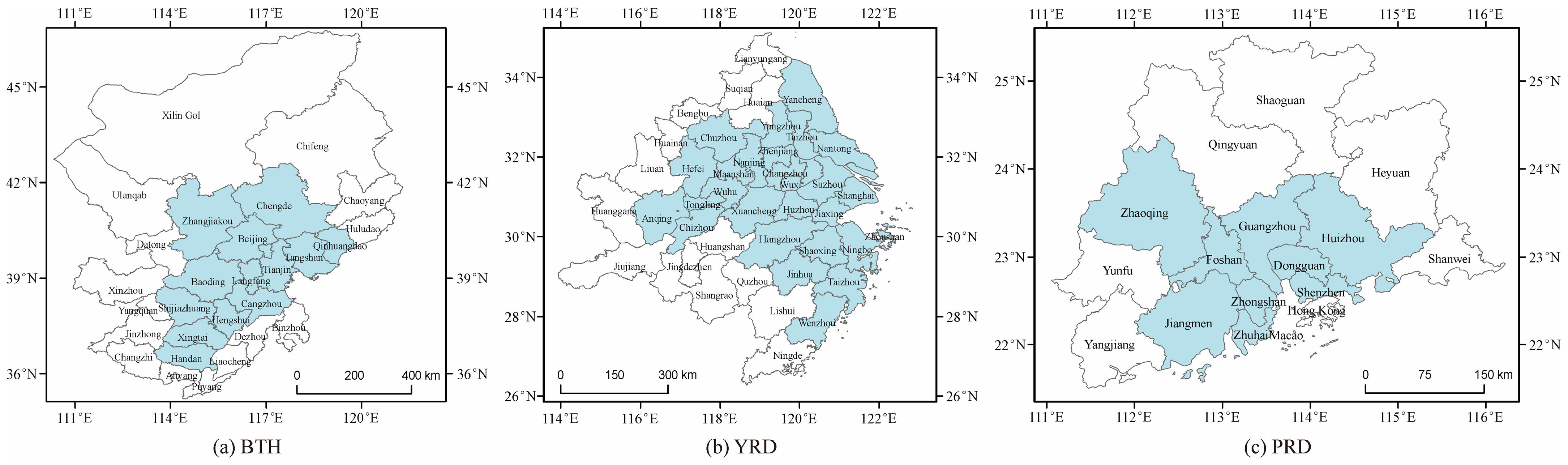
The Beijing–Tianjin–Hebei (BTH) urban agglomeration (blue areas in Figure 1a), which is a densely populated, economically advanced yet heterogeneous core region in northern China, exhibits rapid economic growth and serves as a key national industrial base. However, this rapid economic expansion is accompanied by significant carbon emissions. Research indicates that the region has among the highest carbon emission intensities in China, with emissions demonstrating pronounced spatial clustering, particularly around major urban centers such as Beijing, Tianjin, Tangshan, and Shijiazhuang. The Yangtze River Delta (YRD) urban agglomeration (blue areas in Figure 1b), which encompasses 41 cities at prefecture level and above—including Shanghai and parts of Jiangsu, Zhejiang, and Anhui provinces—is one of China’s most economically developed and urbanized regions. Centered on the estuary of the Yangtze River and leveraging the “Golden Waterway” and coastal port networks, the YRD features a distinctive river–sea–land intermodal transport system. It supports approximately 16% of China’s population and contributes about a quarter of the national GDP, making it a paradigmatic high-density urban-industrial agglomeration. The Pearl River Delta (PRD) urban agglomeration (blue areas in Figure 1c), located in central–south Guangdong Province and comprising nine cities, including Guangzhou, serves as a pivotal economic hub in southern China. Significant intra-regional disparities persist, where the “Four Major Economic Powerhouses” (Guangzhou, Shenzhen, Foshan, and Dongguan) substantially outperform the other cities. As a rapidly developing, densely populated, and energy-intensive region, the PRD is a critical area for implementing emission reduction policies. Thus, research on carbon emissions in the PRD is pivotal for policy design and demonstration.

2.2. Methods

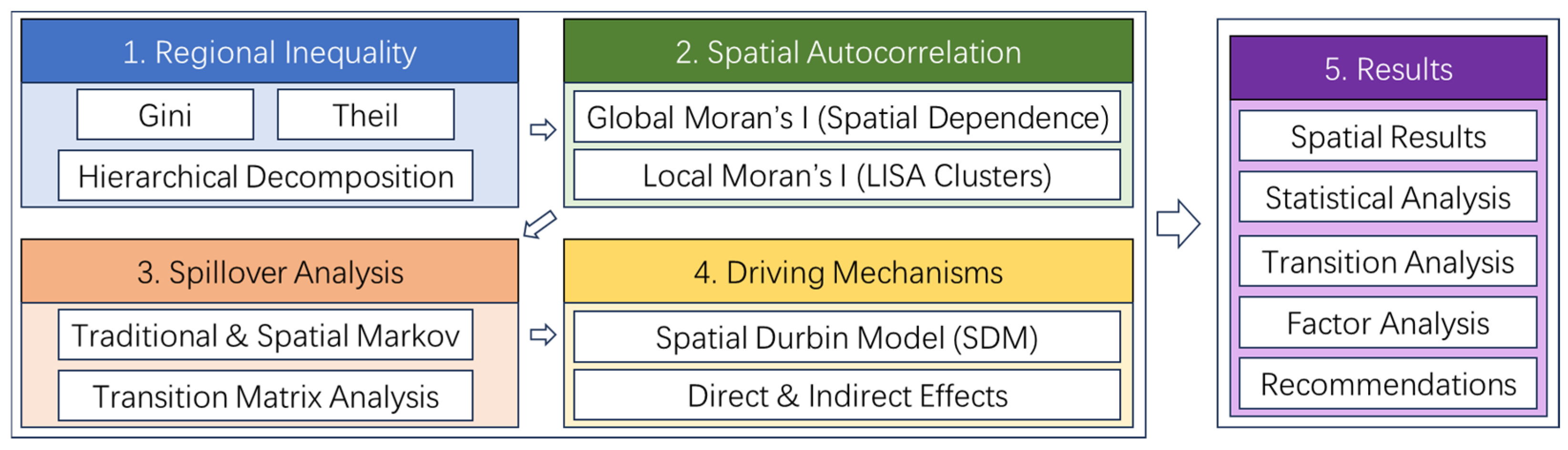
A comprehensive methodological framework that includes the Gini index, the Theil index, Moran’s I, spatial Markov chains, and a Spatial Durbin Model (SDM) is used to quantify emission heterogeneity, spatial spillovers, and their multi-scale drivers in this paper (Figure 2). This study employed a multi-stage analytical approach to examine regional carbon emission patterns. First, regional disparities were quantified and decomposed using the Gini and Theil indices. Next, spatial clustering and heterogeneity were assessed through global and local Moran’s I analysis. Subsequently, spatial Markov chains were applied to model dynamic state transitions and neighborhood spillover effects. Finally, the Spatial Durbin Model (SDM) was utilized to disentangle the direct and indirect effects of key socioeconomic drivers on emissions.

2.2.1. Gini Index

In regional disparity analyses, the Gini index is a fundamental metric. It quantifies inequality by measuring the ratio of the area between the Lorenz curve and the line of perfect equality to the total area under the line of perfect equality [34]. It is mathematically derived from the ordered cumulative distribution of the variable of interest and can be expressed as

$$G={\displaystyle \frac{\sum _{i=1}^n{\sum }_{j=1}^n\left|x_i-x_j\right|}{2n^2\overline{x}}}$$

(1)

where G is the Gini index, $x_i$ and $x_j$ are the variable values for regions i and j, $n$ is the number of regions, and $\overline{x}$ is the mean. The index ranges from 0 to 1, where values close to 0 denote minimal disparity, whereas values near 1 indicate maximal disparity.

2.2.2. Theil Index

The Gini index serves as a robust measure of overall regional disparities, but it does not readily allow for the decomposition of their underlying sources. Therefore, this study employs the Theil index, which decomposes regional inequality into within-group and between-group components using information entropy, thereby providing a more refined decomposition of the structure of inequality [35]. The index is expressed as

$$T={\sum }_{I=1}^G{p}_i\log {\displaystyle \frac{p_i}{v_i}}$$

(2)

where G denotes the number of groups, $p_i$ represents either the population share or the economic weight of group i, and $v_i$ indicates the ratio of the group-specific mean to the overall mean. In addition to providing an aggregate measure of disparity, the Theil index is additively decomposable, breaking down total inequality into within-group and between-group components. This decomposition allows for the precise identification of regional divergence and provides a solid foundation for targeted policy design.

2.2.3. Spatial Auto-Correlation

The global Moran’s I index is used to characterize the overall spatial association and quantify aggregate spatial heterogeneity in both the level and efficiency of urban carbon emissions [36]. Its mathematical expression is

$$I={\displaystyle \frac{\mathrm{n}\sum _{i=1}^n\sum _{j=1}^n{\mathrm{w}}_{ij}\left({\mathrm{y}}_i-\overline{y}\right)\left({\mathrm{y}}_{\mathrm{j}}-\overline{y}\right)}{\sum _{i=1}^n\sum _{j=1}^n{\mathrm{w}}_{ij}\sum _{i=1}^n{\left({\mathrm{y}}_i-\mathrm{y}\right)}^2}}$$

(3)

where n is the total number of prefecture-level cities; yᵢ and yⱼ denote the carbon emissions of city i and city j, respectively; $\overline{y}$ represents the average carbon emission across all prefecture-level cities; and w denotes the spatial weight matrix constructed using Rook contiguity. Moran’s I ∈ [−1, 1], where values approaching 1 indicate strong positive spatial clustering of regions with either high or low carbon emissions.

Global spatial autocorrelation assumes spatial homogeneity and therefore cannot explicitly reveal local clustering structures. Moreover, when the sample size is small (N < 30), the global Moran’s I test based on an asymptotic distribution suffers from a substantial loss of statistical power, increasing the probability of Type II errors in testing spatial independence. Therefore, conclusions should be drawn in conjunction with local indicators of spatial association (LISA) and spatial regression models such as SAR or SDM to avoid misleading inferences from relying on a single method. Local spatial autocorrelation measures the association between each prefecture-level city and its contiguous neighbors; the local Moran’s I is calculated as

$$I_i=z_i\sum _{i\ne j}^{\mathrm{n}}{w}_{ij}{z}_j$$

(4)

where n is the total number of prefecture-level cities, $w_{ij}$ denotes the spatial weight between regions i and j; Zᵢ and Zⱼ are the standardized carbon emission efficiencies (using Z-scores) of regions i and j, respectively; and Iᵢ is the local Moran’s I for region i. A positive (negative) value indicates spatial clustering of similar (dissimilar) attribute values, with larger absolute values indicating stronger clustering intensity.

2.2.4. Markov Model

The Markov chain framework is employed to model cross-regional interactions in carbon emission states. Cities are first classified into three exhaustive and mutually exclusive categories—high, medium, and low—based on per capita emissions [37]. A transition probability matrix is constructed to quantify annual shifts between these states, thereby facilitating the identification of dynamic evolution trends in emission levels. Each element in this matrix represents the probability that a city transitions from one defined emission tier to another over a specified period. Within the Markov chain framework, the initial distribution of cities across emission tiers and the transition probability matrix at a given time enable the forecasting of future emission-level distributions. Let m_ij (t) denote the probability that a city’s per capita carbon emission level transitions from class i to class j between year t and t + 1. The relationship between the probability matrices of two consecutive years can be expressed as

$$R_{t+1}=M\times R_t$$

(5)

This study adopts the spatial Markov approach, which extends classical Markov chains by incorporating a spatial dimension. A spatially conditioned transition probability matrix is constructed to account for neighborhood spillover effects, resulting in a spatial Markov transition matrix. This method explicitly considers the carbon emission levels of neighboring cities in estimating the transition probabilities for a given city. Specifically, the spatial Markov methodology integrates Markov chains with spatial lag analysis, decomposing the conventional transition matrix into a set of conditionally structured transition matrices. Let $m_{ijt}$(k) denote the probability that a city’s carbon emission category transitions from i to j in year t + 1, conditional on the spatial lag of per capita carbon emissions being in category k in year t. Systematic deviations between the conventional and spatially conditioned transition probabilities provide a quantitative measure of the strength of carbon emission linkages between neighboring cities. A statistically significant difference between these probabilities indicates the presence of spatial spillover effects, whereas their alignment suggests an absence of substantial inter-regional influence. To ensure comparability of carbon emission levels across regions, the analysis is conducted using per capita indicators [38].

2.2.5. Spatial Panel Models

Spatial panel models integrate both spatial and temporal dimensions, enabling accurate characterization of spatial linkages and dynamic evolution in carbon emissions across cities and urban agglomerations, while significantly improving the reliability of parameter estimation [39,40]. Throughout the development of cities and urban agglomerations, carbon emissions are influenced not only by local factors—such as industrial structure and technological innovation—but also by complex spatial spillover effects arising from inter-city capital flows, technology diffusion, and population mobility. To capture these mechanisms, the following empirical model is specified:

$$Y_{it}=\beta X_{it}+\rho \sum _{j=1}^N{W}_{ij}{Y}_{jt}+\phi \sum _{j=1}^N{W}_{ij}{X}_{ij}+v_t+{\mu }_t+V_{it}$$

(6)

$$V_{it}=\lambda E{V}_{it}+{\epsilon }_{it}$$

(7)

where $Y_{it}$ denotes the carbon emissions of urban agglomeration i in year t. $X_{it}$ represents a vector of explanatory variables, including industrial structure, technological innovation, population density, and other socioeconomic drivers. The coefficient $\rho$ captures the spatial lag effect, reflecting the marginal influence of emissions from neighboring agglomerations on the local unit. $W_{ij}$ denotes the spatial weight matrix, which quantifies the connectivity strength between city or cluster i and j. $\beta$ is the parameter vector associated with the explanatory variables, and φ is the spatial error coefficient. $v_t$ accounts for time-fixed effects, ${\mu }_t$ represents city-fixed effects. $V_{it}$ denotes the idiosyncratic error term. λ is the spatial autocorrelation coefficient of the error term, and E symbolizes the spatial weighting applied to the disturbance term.

If φ = 0 and β = 0, the specification reduces to the Spatial Error Model (SEM), which accounts for spatial correlation in the disturbance term, thereby representing unobserved, spatially dependent factors. If φ = 0 and λ = 0, the Spatial Lag Model (SLM) is obtained, emphasizing the direct effect of neighboring regions’ carbon emissions on the local region. When λ = 0, it results in the Spatial Durbin Model (SDM); this model incorporates spatial lags of both the dependent and independent variables, thus providing a comprehensive representation of the determinants and spatial propagation mechanisms of carbon emissions.

2.3. Data Source

We employed a carbon emission dataset constructed by Chen et al. [41], which integrates multi-source remote sensing data with ground-based monitoring measurements. The estimates demonstrate consistency with nationally reported carbon emission trends and have been cross-validated in subsequent peer-reviewed studies. In the present study, to extend the series to 2020, an ARIMA model was applied to the available data. The optimal parameters were determined by minimizing the Akaike Information Criterion following Ning et al. [42]. Population grids were obtained from the LandScan Global Dynamic Population Database (https://landscan.ornl.gov/), while socioeconomic indicators were primarily compiled from the China City Statistical Yearbook and corresponding provincial and municipal statistical yearbooks. The data sources above are listed in

Table 1. List of data sources.

Data Name	Source/Description
Carbon Emission Data	Based on Chen et al. [41] and extend to 2020
Population Grid Data	https://landscan.ornl.gov/
Socioeconomic Indicators	China City Statistical Yearbook and provincial/municipal statistical yearbooks

. For prefecture-level cities (or leagues) not covered in the yearbooks, missing data were supplemented using information released in local government statistical bulletins. The remaining missing values were addressed through a two-step procedure: (1) linear interpolation was used to fill isolated annual gaps within otherwise complete city-level series; (2) in the rare cases where data for a specific indicator were entirely missing for a given city and year, the values were imputed using a spatial adjacency-weighted average of the same indicator from neighboring cities, with weights assigned based on inverse geographical distance or administrative proximity.

Following the established literature, we operationalized the spatial panel model by selecting seven socioeconomic proxy variables to examine their effects on energy-related carbon emissions [43,44,45]. (1) Economic growth (x₁) is measured by per capita GDP. Previous evidence indicates that cities experiencing rapid economic expansion, characterized by high industrial output and household consumption, possess greater fiscal capacity to invest in environmentally friendly technologies. (2) Technological level (x₂) is proxied by per capita government expenditure on science and technology, which reflects the local authorities’ commitment to energy-saving research and development. (3) Urban population scale (x₃) is quantified by population density (persons km⁻²), since denser urban areas exhibit higher baseline energy demands for daily activities such as electricity, heating, and transportation. (4) Fixed-asset investment share (x₄) serves as a proxy for the prevailing urban-development paradigm. In most cities, particularly resource-based ones in Central and Western China, investment-driven growth has led to significantly elevated energy consumption. (5) Industrial structure (x₅) is represented by the share of the secondary sector, which underscores the disproportionate contribution of heavy industries such as steel and chemicals, which continue to be the primary sources of carbon emissions. (6) Economic openness (x₆) is gauged by foreign direct investment achieved per capita, as inward FDI may promote the adoption of energy-efficient technologies. (7) Road-network density (x₇) is proxied by per capita road area; enhanced road infrastructure helps alleviate congestion-related emissions [46].

3. Results

3.1. Spatial Analysis of Carbon Emission

3.1.1. Statistical Analysis

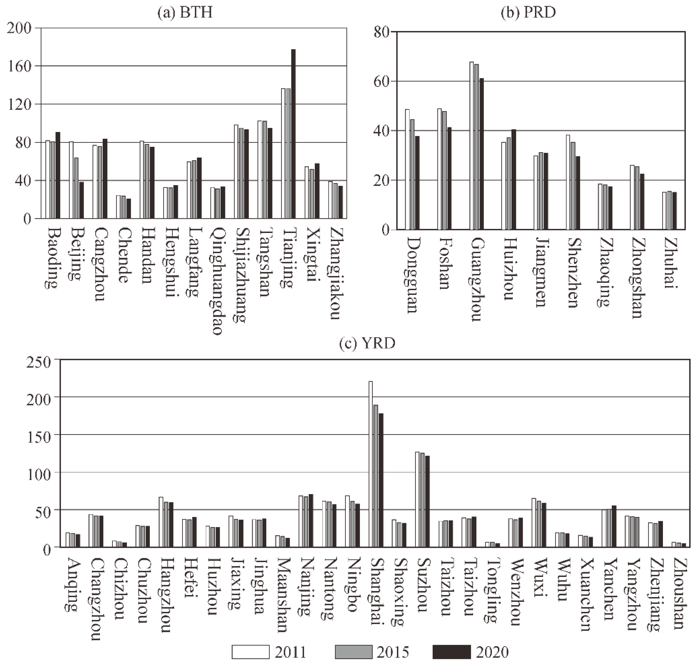
We first analyze the emission inventories of the three urban agglomerations from 2011 to 2020 (as shown in Figure 3). Total emissions from the BTH, YRD, and PRD regions have experienced a sustained decline, though with notable regional heterogeneity. Overall, industrial cities within the BTH region contribute a relatively high proportion of emissions. In particular, Beijing has achieved significant emission reductions through policy interventions. Chengde and Zhangjiakou also exhibit downward trends in total emissions. By contrast, heavily industrialized cities such as Tangshan, Shijiazhuang, and Tianjin maintain high emission levels. Notably, emissions in Tianjin in 2020 were 28.3% higher than the 2015 level. The remaining cities in the BTH region continue to exhibit medium-to-high emission intensities, highlighting considerable intra-regional heterogeneity.

In comparison with BTH, cities in the PRD demonstrate lower total emissions. Guangzhou, where traditional manufacturing remains a substantial component of the economy, recorded the highest emissions in the region, though still below 70 Mt—approximately half of Tianjin’s total. Declining emission trajectories are observed in cities such as Shenzhen, Dongguan, Foshan, Zhuhai, and Zhaoqing. Shenzhen has achieved substantial emission reductions through industrial upgrading and relocation, highlighting the region’s potential for mitigation. Conversely, Huizhou, which absorbed relocated industries (particularly electronics) from other cities, experienced a 13.9% increase in emissions in 2020.

In the YRD region, the highest emitters are concentrated along the Shanghai–Nanjing and Shanghai–Hangzhou corridors, including Shanghai, Suzhou, Wuxi, Nanjing, Nantong, Ningbo, and Hangzhou. Most of these cities display a trend of emission reduction, while peripheral cities surrounding them show an expansion in carbon emissions. This pattern suggests that core cities such as Shanghai and Suzhou have curbed emissions through industrial restructuring, whereas peripheral cities like Hefei and Yancheng have undergone emission growth due to the spatial transfer of relocated industries.

3.1.2. Spatial Analysis

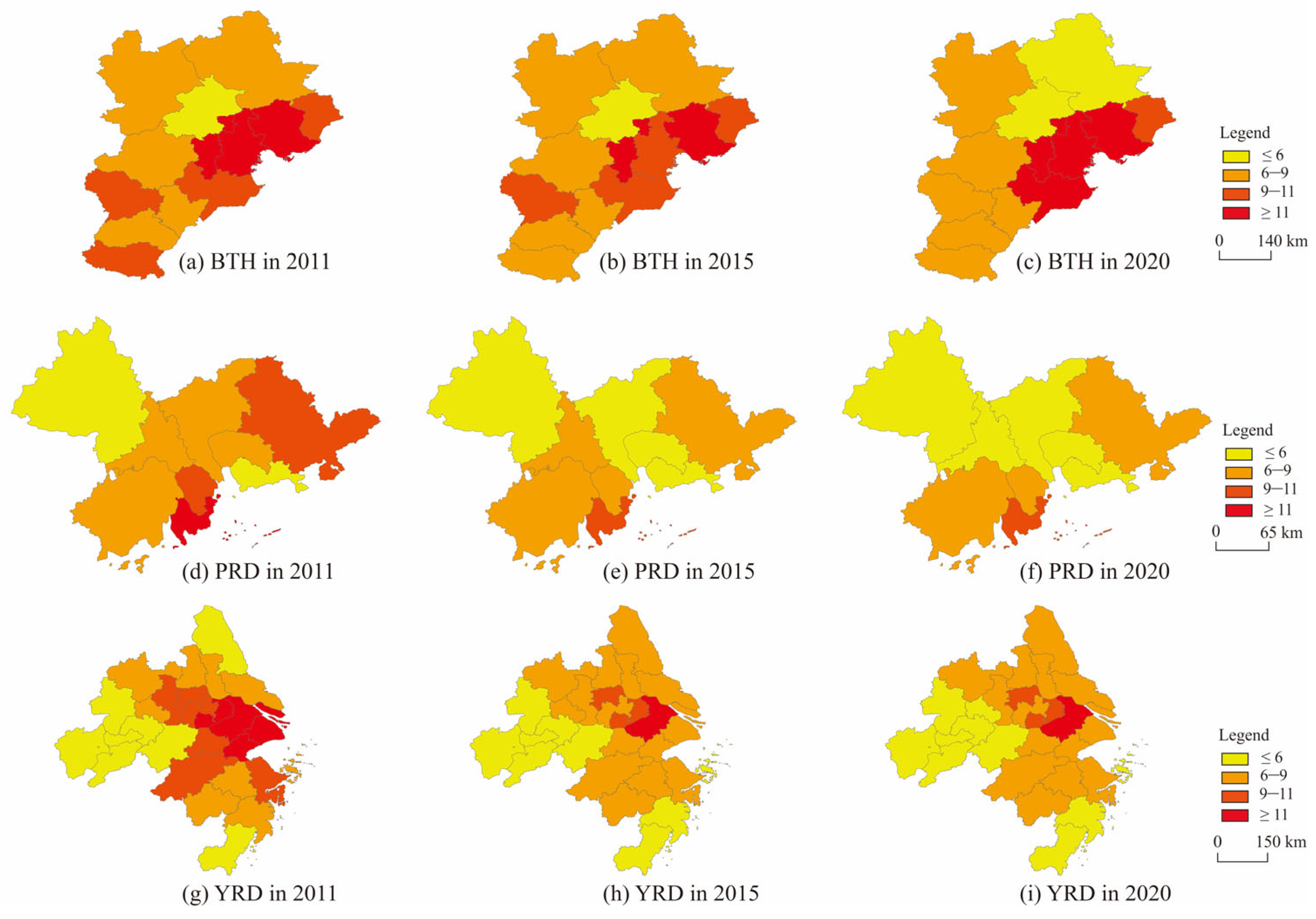
We also analyzed the per capita carbon emission patterns across the three urban agglomerations (Figure 4). In the BTH region, cities with high per capita emissions are predominantly concentrated around Bohai Bay, indicating significant regional inequality. For example, Langfang—a manufacturing-oriented city—exhibits a per capita emission intensity several times higher than that of Beijing, the metropolitan core. This substantial gap between industrial cities and central urban areas (e.g., Beijing) reflects a structural contradiction between population scale and resource consumption within industrial agglomerations.

By contrast, the PRD region exhibits more substantial overall reductions in per capita emissions. Core cities, including Guangzhou, Shenzhen, Dongguan, and Foshan, have successfully reduced their per capita carbon emission intensity through industrial relocation and technological upgrading. However, cities such as Huizhou and Jiangmen continue to depend on conventional development pathways by accommodating industries relocated from core urban areas.

In the YRD region, per capita emission intensity shows an overall declining trend, particularly in formerly high-emission zones. Core cities, such as Shanghai, achieved notable reductions in per capita emissions through industrial structure optimization, especially during the period from 2011 to 2015. Furthermore, statistical analysis indicates that Taizhou and Yancheng, affected by industrial relocation, experienced increased per capita emissions due to technological path dependence, highlighting how industrial relocation can lead to spatial substitution effects.

3.1.3. Gini Index and Theil Index

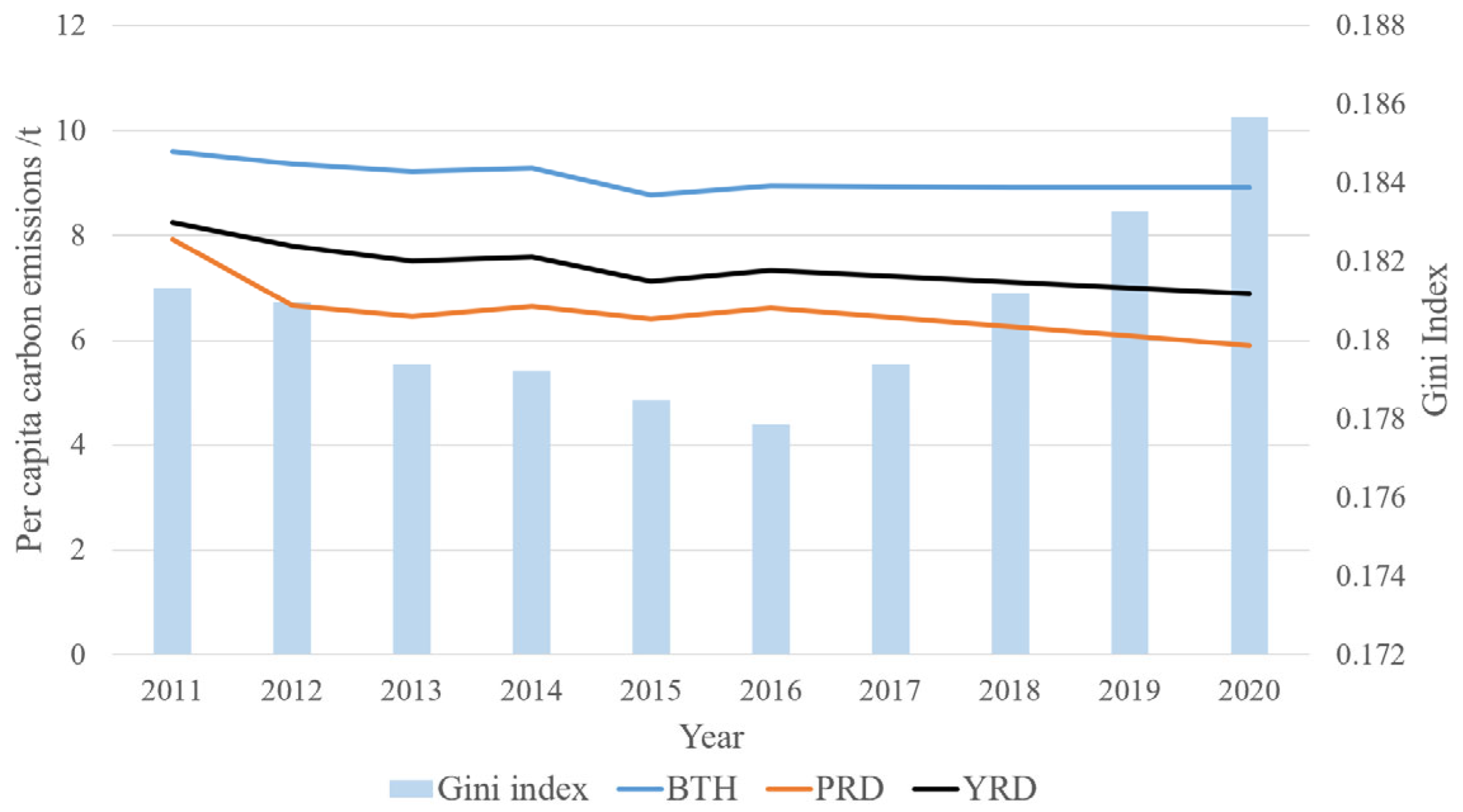
The three urban agglomerations demonstrate notable spatial heterogeneity in both total carbon emissions and per capita emission intensity. To quantify these disparities, we calculated time-series Gini indexes (Figure 5). The inter-agglomeration Gini index increased slightly from 0.181 to 0.186 (a rise of 2.4%), indicating a relatively modest expansion in inequality. Notably, the BTH region consistently recorded the highest annual per capita carbon emissions while exhibiting the smallest decline (7.1%), including a temporary rebound to 9.28 tons in 2014. This volatility arises from the combined effect of the dominance of heavy industries (e.g., steel and chemicals) and a slow energy transition. In contrast, the YRD and PRD regions achieved significant reductions in per capita emissions, of 16.5% and 25.6%, respectively. These improvements are associated with industrial restructuring (e.g., the expansion of the service sector), coordinated environmental governance (e.g., integration policies in the YRD), and technological innovation.

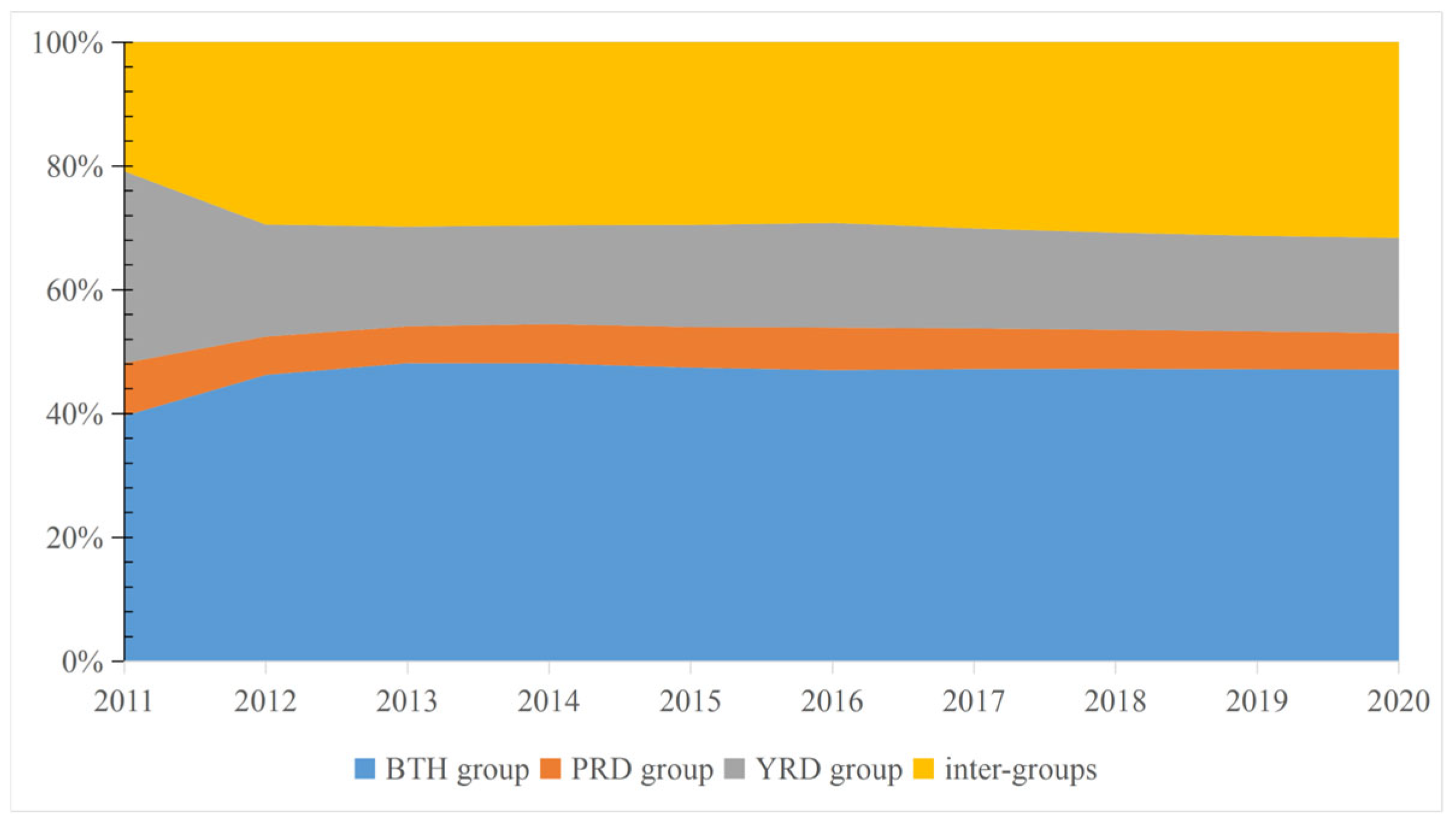
Decomposition of the Theil index reveals that intra-group disparity, rather than inter-group differences, represents the primary source of regional heterogeneity (Figure 6). Although the contribution of inter-group disparities increased from 20.85% in 2011 to 31.63% in 2020, intra-group disparities still constituted 68.37% of the total in 2020. Thus, imbalances within agglomerations remain the main driver of overall regional inequality in carbon emissions. Among the three agglomerations, the BTH region showed the sharpest increase in intra-group divergence, with its contribution rising from 39.6% to 47.1%. This trend stems from Beijing’s successful transition to service- and high-tech-oriented industries, whereas Hebei remains dependent on energy-intensive manufacturing with a high proportion of coal in its energy mix, thereby widening regional disparities. In contrast, both the YRD and PRD experienced declines in intra-group contributions (from 31.0% to 15.4% and from 8.5% to 5.9%, respectively), indicating more effective regional coordination facilitated by industrial synergy, technology diffusion, and policy alignment.

Rising inter-group Theil indices indicate a growing disparity in emission efficiency among the three urban agglomerations. This divergence is primarily driven by the BTH region’s entrenched industrial structure and inadequate regional coordination mechanisms. Conversely, both the YRD and PRD regions managed to reduce inter-group disparities through market-oriented policies and technological innovation. Since 2017, the Gini index has increased from 0.179 to 0.186, a trend that is closely linked to the BTH’s slower pace of emission reduction. The region’s persistent internal inequality and poor coordination capacity have further exacerbated inter-regional disparities.

3.1.4. Global Moran’s I Test

To examine spatial agglomeration effects of carbon emissions, we performed global Moran’s I analysis of per capita emissions for the three urban agglomerations over 2011 to 2020 using Geoda (version 1.22) spatial statistical software (

Table 2. Global Moran’s I of urban agglomerations.

	2011 (I/P)	2015 (I/P)	2020 (I/P)
BTH	0.099/0.055 *	0.147/0.020 **	0.124/0.045 **
PRD	0.117/0.141	0.160/0.087 *	0.041/0.244
YRD	0.603/0.001 ***	0.675/0.001 ***	0.628/0.001 ***

***, **, and * denote statistical significance at the 1%, 5%, and 10% levels, respectively.

). The results reveal marked heterogeneity in spatial autocorrelation across regions. Spatial clustering within the BTH region intensified markedly, with Moran’s I rising from 0.099 in 2011 to 0.147 in 2015 before easing to 0.124 in 2020. This trajectory indicates that administrative coordination reshapes spatial interactions and drives new clustering patterns. In the PRD region, Moran’s I fluctuated between 0.117 and 0.160 before declining to 0.041. We also found that estimates in 2011 and 2020 are statistically non-significant. The weak spatial dependence reflects the region’s small sample size (n = 15) and rapid diffusion of advanced technologies, with technology spillovers among neighboring jurisdictions driven by market competition. Within the YRD region, Moran’s I remained above 0.60 throughout the study period, reaching 0.675 in 2015, and all estimates are significant at the 1% level. This robust positive spatial autocorrelation suggests that geographical proximity and industrial homogeneity are primary drivers of carbon-emission clustering.

3.1.5. LISA Cluster Analysis

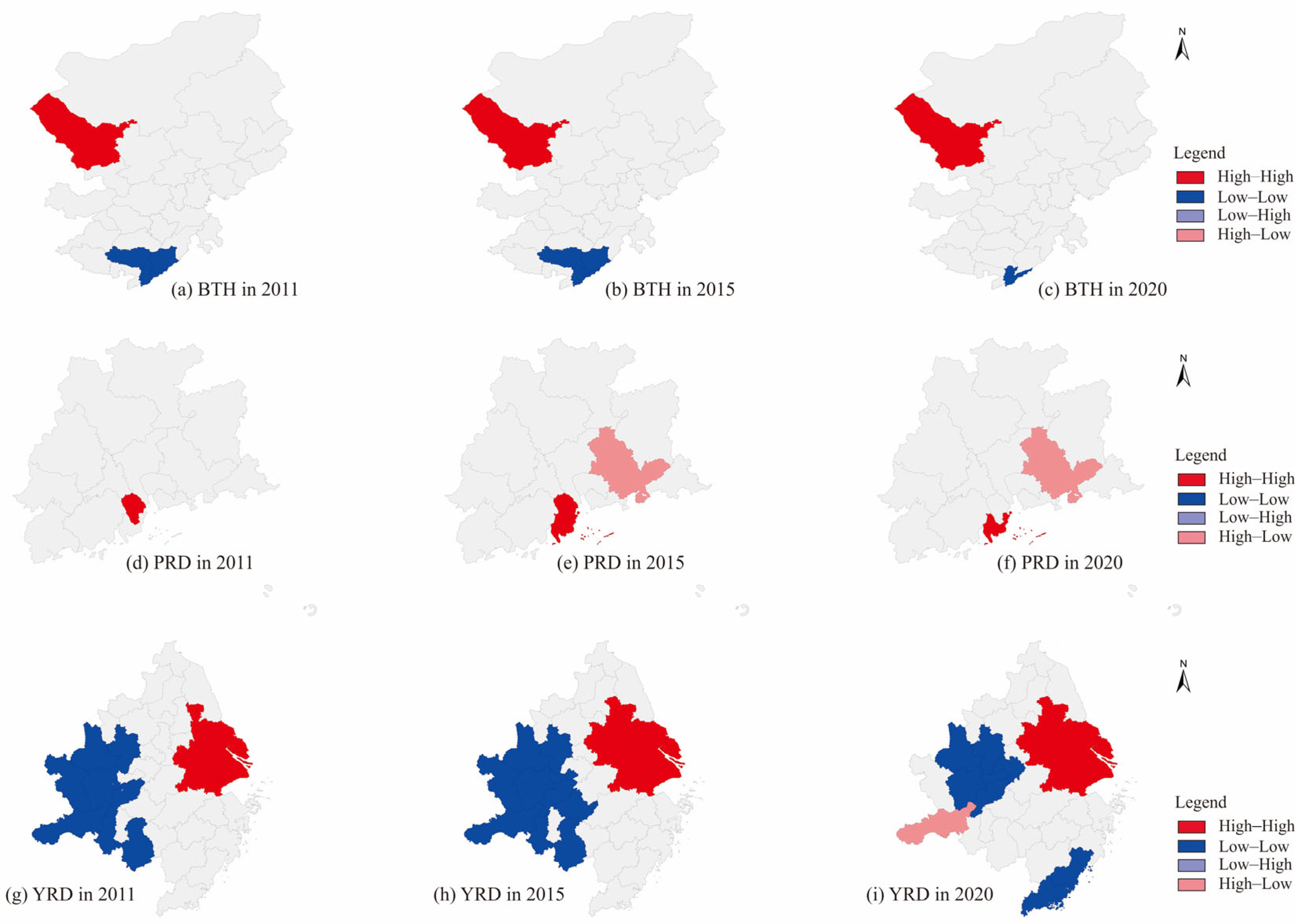
While global spatial autocorrelation reflects overall spatial association patterns, it fails to reveal localized atypical characteristics. To address this limitation, we conducted a local LISA cluster analysis and generated LISA cluster maps (Figure 7). These maps illustrate the spatial clustering of per capita carbon emissions in all three major urban agglomerations in 2011–2020. The results identify significant local spatial autocorrelation in total carbon emissions at the prefectural level. Cities that did not show significant spatial autocorrelation exhibit limited mutual influence with neighboring regions in terms of total carbon emissions, suggesting negligible spillover effects.

The BTH and PRD regions display notable regional heterogeneity, although some areas did not reach the threshold of global significance (p > 0.1). In the BTH region, a fragmented “low-carbon core and high-carbon periphery” pattern can be observed. Industrial decentralization has relocated Beijing’s steel industry to Tangshan, while constraints on population density and coal consumption have collectively contributed to a dilution effect. These factors have collectively widened the emission gap between core and peripheral zones. In the PRD region, economic centers and manufacturing nodes show distinct trends. Guangzhou and Shenzhen have achieved decarbonization through the dominance of high-tech industries and population dilution effects. In contrast, Zhongshan, Zhuhai (HH cluster), and Huizhou (HL cluster) function as local high-emission nodes due to their role in accommodating traditional manufacturing. On the other hand, the YRD region exhibits consistent global and local spatial correlation. The agglomeration of petrochemical and steel industries, coupled with geographical proximity and economic development, has led to the emergence of carbon lock-in effects. This has resulted in persistent High–High clusters along the Shanghai–Suzhou–Nantong Yangtze corridor, as well as in cities such as Liuan and Anqing. Peripheral cities, including Liuan and Anqing, have remained long-term Low–Low zones owing to delayed industrial transfer. Notably, Jiujiang exhibited a High–Low spatial outlier in 2020, suggesting the cross-boundary transfer of high-carbon industries through interprovincial cooperation.

3.2. Analysis of Urban Spatial Spillover Effects

3.2.1. Markov Transition Analysis

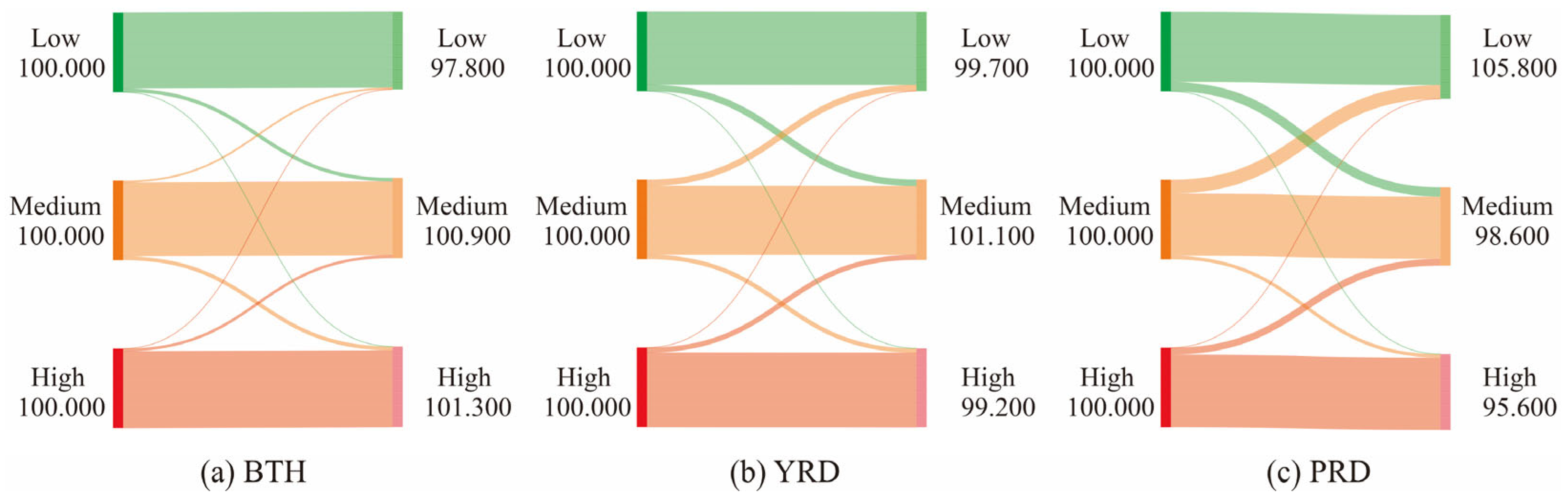
We classified urban per capita carbon emissions into low-, medium-, and high-level types using the tertile approach. Based on temporal data from 2011 to 2020, transition tables can be derived to capture inter-type shifts (quantity ratio) across cities (

Table 3. Transition matrix of per capita carbon emissions.

	BTH			PRD			YRD
	Low	Medium	High	Low	Medium	High	Low	Medium	High
low	0.954	0.046	0.000	0.884	0.116	0.000	0.917	0.083	0.000
medium	0.024	0.927	0.049	0.174	0.783	0.043	0.080	0.864	0.056
high	0.000	0.036	0.964	0.000	0.087	0.913	0.000	0.064	0.936

). In addition, Sankey diagrams (https://sankeymatic.com/build/, accessed on 4 January 2026) are used to represent dynamic transitions over time (Figure 8). The values in Figure 8 represent quantity percentages, distinct from probability percentages. All three urban agglomerations exhibited limited transition dynamics, indicating strong carbon lock-in effects. These systems largely remained in their initial emission categories, with no instances of cross-tier transitions. The BTH region showed the weakest transition dynamics and the strongest degree of carbon lock-in. Conversely, the PRD region exhibited the most significant changes, particularly the highest probability of transitions from medium to high emissions.

Detailed transition probabilities are provided in Table 3. In the BTH region, the self-maintenance probabilities reached 0.953 (low), 0.927 (medium), and 0.964 (high), reflecting the strongest high-emission lock-in among all regions. Notably, the probability of transitioning from medium to high emissions (4.88%) exceeded that of downgrading from medium to low emissions (2.44%). This asymmetry suggests a potential “Matthew Effect” in emission pathways. In the PRD region, the diagonal elements of the transition matrix were substantially higher than the off-diagonal elements. Self-maintenance probabilities were 0.884 (low), 0.783 (medium), and 0.913 (high), indicating notable emission stability and hierarchical rigidity. Transitions occurred exclusively between adjacent levels. The probability of transitioning from medium to low emissions was 17.39%, while that from medium to high emissions was only 4.35%. The YRD region exhibited characteristics of dynamic equilibrium. The self-maintenance probabilities were 0.917 (low), 0.864 (medium) and 0.935 (high). Cities in the medium-emission category showed notable bidirectional mobility: 8.00% transitioned down to low emissions, and 5.60% transitioned up to high emissions. The high-emission category retained relatively weak lock-in properties.

Overall, the agglomerations demonstrated robust self-maintenance tendencies and a strong preference for adjacency-based transitions. The complete absence of cross-tier shifts reflects the presence of path dependence and spatial convergence in urban carbon emission evolution. The BTH region exhibited exceptional stability, with more than 95% retention in the low-emission category and less than a 4% transition out of high emissions, highlighting substantial decarbonization challenges. The PRD region showed the highest persistence of high emissions; however, its risk of transition from medium to high emissions was the lowest (4.35%), suggesting that pressure for low-carbon transition is concentrated mainly in high-emission cities. The YRD region displayed the greatest fluidity among medium-emission cities, with a total transition probability of 13.60%, indicating greater potential for policy interventions to facilitate emission convergence. These distinct structural characteristics provide an empirical basis for designing differentiated carbon emission governance pathways.

3.2.2. Carbon Transfers in Different Neighborhood Environments

To address the inability of traditional models to capture spatial spillover effects and regional heterogeneity, this study constructs spatial Markov transition matrices (

Table 4. Carbon transfers in different neighborhood environments using spatial Markov model.

		BTH			YRD			PRD
		Low	Medium	High	Low	Medium	High	Low	Medium	High
low-carbon neighbor	low	0.955	0.046	0.000	0.821	0.179	0.000	0.930	0.070	0.000
	medium	0.015	0.939	0.046	0.333	0.611	0.056	0.146	0.792	0.063
	high	0.000	0.056	0.944	0.000	0.125	0.875	0.000	0.800	0.200
medium-carbon neighbor	low	0.932	0.068	0.000	0.880	0.120	0.000	0.898	0.102	0.000
	medium	0.032	0.903	0.065	0.135	0.838	0.027	0.077	0.865	0.058
	high	0.000	0.023	0.977	0.000	0.136	0.864	0.000	0.149	0.851
high-carbon neighbor	low	0.962	0.039	0.000	0.902	0.098	0.000	0.750	0.250	0.000
	medium	0.024	0.905	0.071	0.233	0.733	0.033	0.058	0.865	0.077
	high	0.000	0.063	0.938	0.000	0.059	0.941	0.000	0.055	0.945

) by incorporating constraints based on neighboring carbon emission states, which are categorized into three types: low-carbon, medium-carbon and high-carbon environments. As shown in Table 4, the YRD is the most significantly influenced by neighborhood effects. Cities adjacent to low-emission neighbors exhibit an increased probability of transitioning from high to low emissions, while those adjacent to high-emission neighbors show a higher probability of shifting from low to medium emissions. In contrast, the BTH region displays minimal changes in transition probabilities, indicating negligible spatial dependence. The PRD exhibits an opposite trend under low-emission neighborhood conditions, with increased probabilities of transitioning toward high-emission states. These patterns demonstrate the complexity of spatial linkages under geographical adjacency rules. The YRD relies more heavily on geography–economy coupling effects, while BTH’s weak spatial dependence is reinforced by policy interventions. Meanwhile, the PRD’s traditional spatial dependence is weakened by technological diffusion and marketization mechanisms. We also analyze carbon emission transitions under three different neighborhood environments.

In low-emission neighborhood environments, responses to adjacent carbon states vary markedly across agglomerations. In the PRD, the low-emission self-maintenance probability is 0.821, which is 7.0% lower than that in the standard Markov model (0.884), indicating no synergistic emission reduction effect despite intensified low-carbon competition. For the BTH, the low-emission self-maintenance probability remains stable, reflecting regional consistency in low-carbon policy implementation. In the YRD, the high-emission self-maintenance probability drops to 0.2, while the transition probability to medium emissions rises to 0.8. This represents a 73.5% structural deviation from the standard model’s high-emission persistence (0.936). This phenomenon primarily stems from an “emission reduction siphon effect”, whereby low-carbon core cities (e.g., Shanghai) accelerate neighboring high-carbon areas’ transition through technology spillovers and industrial restructuring. Additionally, synergistic mechanisms in regional carbon markets prompt high-emission enterprises to proactively optimize emission strategies under low-carbon competitive pressure, while infrastructure sharing within the core-periphery structure weakens path dependence in high-emission areas.

Under medium-emission neighborhood conditions, the YRD’s probability of transitioning from medium to high emissions is 0.063, slightly higher than that in the standard Markov model (0.056) but significantly lower than those of the PRD (0.056) and BTH (0.046), suggesting that industrial-chain carbon transfer is constrained by regional policies. In the PRD, the medium-emission self-maintenance probability decreases to 0.611 under medium-emission neighborhood conditions compared to 0.783 in the standard model, indicating intensified pressure for industrial transformation.

In high-emission neighborhood environments, BTH’s high-emission self-maintenance probability is 0.938, lower than that in the standard model (0.963), confirming the regulatory role of its administratively driven governance. The YRD and PRD exhibit similar probabilities (0.945 and 0.941, respectively), demonstrating that high-carbon pathways are susceptible to inter-regional economic linkages. Examples include the PRD’s reliance on external high-carbon export industries within its export-oriented economy, and the YRD’s regional coordination in heavy/chemical industries affecting the stability of high-emission cities.

4. Discussion

4.1. Spillover Effects Analysis Using Spatial Econometric Model

Given data heterogeneity, a logarithmic transformation was applied to normalize the dataset. To select among the Spatial Lag Model (SAR), Spatial Error Model (SEM), and Spatial Durbin Model (SDM), a multi-model diagnostic testing procedure was conducted. This procedure incorporated Lagrange Multiplier tests for spatial lag (LM-lag) and spatial error (LM-error), as well as Wald tests and Likelihood Ratio (LR) tests. As summarized in

Table 5. Spatial panel model test results.

Urban Agglomerations	Models
	SAR or SEM?		Should the SDM Be Reduced?
	LM-Lag	LM-Error	Wald-Lag	Wald-Error	LR-Lag	LR-Error
BTH	6.959 ***	22.072 ***	5.520	25.950 ***	109.201 ***	105.813 ***
PRD	30.296 ***	62.053 ***	19.662 ***	75.152 ***	138.570 ***	132.324 ***
YRD	20.404 ***	8.691 ***	34.490 ***	42.893 ***	109.763 ***	167.165 ***

*** denotes statistical significance at the 1%.

, the test statistics for both LM-lag and LM-error were significant at the 1% level across all three urban agglomerations, confirming the presence of both spatial lag and spatial error effects and thus supporting the applicability of SAR and SEM frameworks. To evaluate whether the SDM could be simplified to the SAR or SEM, Wald and LR tests were further conducted. Both tests rejected the null hypothesis of reducibility (p < 0.01), indicating that the SDM incorporates spatial dependence features not fully captured by SAR or SEM. Consequently, the Spatial Durbin Model (SDM) was selected for final parameter estimation.

4.2. Explanations Based on SDM

We conducted analyses using SDM with temporal fixed effects, individual fixed effects, and spatiotemporal fixed effects. Across all urban agglomerations, the model with temporal fixed effects consistently exhibited the highest goodness-of-fit, significantly outperforming the other two specifications. For example, within the PRD agglomeration, the temporal fixed effects model achieved an R² of 0.623, whereas the individual fixed effects and spatiotemporal fixed effects models exhibited substantially lower R² values, at only 0.012 and 0.023, respectively.

Based on these findings, we selected the SDM with temporal fixed effects to obtain the parameter estimates, t-statistics, and significance (

Table 6. Parameter estimation based on SDM.

	BTH		PRD		YRD
	Coefficient	t	Coefficient	t	Coefficient	t
Economic growth (x1)	0.387 ***	6.272	0.556 ***	8.319	0.267 ***	10.533
Technology (x2)	−0.124 ***	−3.814	−0.076 ***	−2.826	0.037 ***	2.594
Population scale (x3)	−0.146 ***	−5.352	−0.185 ***	−6.54	−0.058 ***	−2.911
Fixed investment (x4)	−0.013	−0.341	−0.013	−0.276	−0.045 *	−1.705
Industrial structure (x5)	0.743 ***	7.960	0.582 ***	7.182	−0.115 **	−2.124
Opening up (x6)	0.064 ***	4.159	−0.005	−0.274	0.034 ***	3.477
Road density (x7)	0.198 ***	4.337	0.207 ***	4.812	0.189 ***	8.289
R2	0.718		0.623		0.566

***, **, and * denote statistical significance at the 1%, 5%, and 10% levels, respectively.

). The goodness-of-fit results indicate that all urban agglomerations attained R² values exceeding 0.5, suggesting a reasonably strong model fit. Specifically, the model demonstrated the highest explanatory power for the Beijing–Tianjin–Hebei (BTH) agglomeration (R² = 0.718), followed by the PRD agglomeration (R² = 0.623). The Yangtze River Delta (YRD) agglomeration also displayed a robust fit, with an R² of 0.566.

Analysis of the parameter estimates revealed significant differences in the driving factors of carbon emissions among the three agglomerations. The scale effect of economic growth (x₁) was strongest in the PRD (0.556), which can be attributed to manufacturing expansion in cities such as Dongguan and Foshan, leading to increased energy consumption. This effect was weaker in the YRD (0.267), potentially due to the growing service sector share in Shanghai and Hangzhou. The BTH agglomeration (0.387) exhibited a relatively strong effect, possibly supported by inter-regional infrastructure development. The impact of technology investment (x₂) varied across regions. It was associated with a slight increase in emissions in the YRD (0.037), potentially linked to technological advances in the electronics and chemical industries. In contrast, technology investment contributed to emission reductions in the PRD (−0.076) and BTH (−0.124) regions, likely resulting from green innovation initiatives. Population density (x₃) had the most substantial emission-reducing effect in the PRD (−0.185), benefiting from rail transit connectivity between Guangzhou and Shenzhen as well as spatially intensive development. In the BTH region (−0.146), emission reduction was driven by industrial decentralization in Beijing and population management policies. We found that fixed investment (x₄) had an insignificant effect on carbon emissions. We speculate that this may be due to the correlation between fixed investment and other explanatory variables (such as economic development, industrial structure, etc.), making it difficult for the model to isolate its independent contribution. The proportion of secondary industry (x₅) highlights regional disparities in industrial transition. The YRD showed a significant negative effect (−0.115), reflecting a successful transition toward high-end manufacturing. In contrast, the PRD (0.582) and BTH (0.743) regions continued to be influenced by their reliance on traditional industries. Foreign capital utilization (x₆) contributed to increased emissions in both the YRD (0.034) and BTH (0.064) agglomerations. Its effect in the PRD was statistically insignificant, a difference that may be related to variations in the quality of foreign investment. An increase in per capita road area (x₇) exerted a positive influence on carbon emissions across all three major agglomerations, with coefficients ranging from 0.189 to 0.207. This highlights the common challenge of mitigating emissions from transportation infrastructure.

4.3. Effect Decomposition

To elucidate the internal and cross-regional mechanisms, this study decomposed the spatial effects into direct and indirect components for each urban agglomeration (

Table 7. Decomposition of spatial spillover effects of different urban agglomerations.

Variables	BTH		PRD		YRD
	Direct (Coefficient/[t])	Indirect (Coefficient/[t])	Direct (Coefficient/[t])	Indirect (Coefficient/[t])	Direct (Coefficient/[t])	Indirect (Coefficient/[t])
Economic growth (x1)	0.383 *** [6.013]	−0.279 * [−1.749]	0.532 *** [8.523]	1.062 *** [5.855]	0.272 *** [10.962]	0.110 ** [2.166]
Technology (x2)	−0.123 *** [−3.726]	0.107 [1.239]	−0.080 *** [−3.024]	0.071 [1.357]	0.031 ** [2.257]	−0.129 *** [−3.006]
Population Scale (x3)	−0.145 *** [−5.673]	−0.06 [−1.242]	−0.180 *** [−6.466]	−0.107 [−1.391]	−0.051 *** [−2.648]	0.108 * [1.749]
Fixed investment (x4)	−0.012 [−0.330]	0.022 [0.205]	0.001 [0.022]	−0.608 *** [−4.849]	−0.035 [−1.435]	0.252 *** [2.954]
Industrial structure (x5)	0.732 *** [7.789]	−0.524 ** [−2.385]	0.592 *** [7.630]	−0.628 *** [−2.701]	−0.164 *** [−3.160]	−1.050 *** [−5.839]
Opening up (x6)	0.064 *** [4.253]	−0.039 [−0.936]	−0.004 [−0.243]	0.006 [0.167]	0.037 *** [3.802]	0.046 ** [2.076]
Road density (x7)	0.194 *** [4.058]	−0.18 [−1.643]	0.200 *** [4.780]	0.234 ** [2.538]	0.209 *** [8.818]	0.421 *** [5.874]

***, **, and * denote statistical significance at the 1%, 5%, and 10% levels, respectively.

). The analysis revealed significantly positive direct effects of GDP per capita (x₁) in the BTH (0.383), PRD (0.532), and YRD (0.272) agglomerations, indicating that economic growth primarily drives carbon emissions via local scale effects within each region. However, the spatial spillover patterns diverged substantially. Both the YRD and PRD exhibited significantly positive indirect effects (0.110 and 1.062, respectively), suggesting that economic synergy contributes to higher regional emissions. In contrast, the BTH agglomeration exhibited a significantly negative indirect effect (−0.279), which primarily stems from competitive emission reduction policies that suppress emissions in neighboring regions.

Technology investment (x₂) exhibited contrasting mechanisms across regions. In the YRD, a significantly positive direct effect (0.031) was accompanied by a significantly negative indirect effect (−0.128), implying that local technological advancement in the area not only increases its own emissions but also facilitates emission reduction in adjacent areas. Both the PRD and BTH regions showed significantly negative direct effects (−0.080 and −0.123, respectively), confirming the local mitigating impact of green technology. However, neither region exhibited statistically significant spatial spillovers. Population density (x₃) consistently showed negative direct effects across all agglomerations (ranging from −0.051 to −0.145). In terms of indirect effects, the YRD demonstrated significantly positive spillovers (0.108), suggesting that industrial relocation and population mobility export emission pressures to neighboring areas. By contrast, the PRD and BTH showed insignificant or weakly negative indirect effects, highlighting that intensive development enhances regional capacity for emission control. Fixed asset investment (x₄) generated a significantly positive indirect effect in the YRD (0.252). This may occur when regional green investments displace low-carbon resources in neighboring areas, inadvertently incentivizing high-carbon investments there. The share of the secondary industry (x₅) had the most pronounced impact. In the YRD, both direct and indirect effects were significantly negative (−0.164 and −1.050, respectively), demonstrating that industrial modernization not only reduces local emissions but also curbs high-carbon activities in neighboring areas through industrial synergy. Conversely, the PRD and BTH exhibited significantly positive direct effects (0.592 and 0.732) coupled with significantly negative indirect effects (−0.628 and −0.524), indicating a continued local reliance on high-carbon industrialization, while regional competition drives emission reductions in adjacent regions. Foreign capital utilization (x6) produced significantly positive direct effects in both the YRD (0.037) and BTH (0.064). It also had a significantly positive indirect effect in the YRD (0.046), suggesting that foreign investment increases both local and regional emissions. The insignificant impact in the PRD implies a higher prevalence of quality foreign investment in that region. The per capita road area (x7) showed significantly positive direct effects across all agglomerations, as well as significantly positive indirect effects in the YRD and PRD. These results indicate that transport network expansion increases emissions through improved regional connectivity. However, the BTH region displayed a significantly negative indirect effect (−0.180), likely due to strategic traffic resource allocation policies.

4.4. Differentiated Strategies for Urban Agglomerations

The key findings of this study inform a framework of actionable mitigation strategies tailored to the distinct characteristics of each major urban agglomeration.

For the Beijing–Tianjin–Hebei (BTH) region, the critical objective is to overcome carbon lock-in. We propose an administrative coordination–industrial restructuring strategy. This recommendation is grounded in three findings: BTH exhibits the highest intra-regional disparity contribution (47.1%), demonstrates strong persistence in high-emission states (0.964), and shows a negative spatial spillover from economic growth (−0.279). The latter indicates that growth in one area may suppress emissions in neighboring regions, suggesting competitive dynamics. To address this, we recommend two actions. First, establish a cross-jurisdictional green restructuring mechanism for heavy industries. This should involve creating mandatory Regional Carbon Intensity Access Standards for Steel and Chemical Industry Transfers, leveraging Beijing’s technological capacity and Hebei’s industrial base. A supporting regional green technology fund would ensure decarbonization accompanies physical relocation. Second, transform competitive mitigation into collaborative action. Policymakers can utilize the observed negative spillover by piloting an Integrated Regional Carbon Budget scheme for key industrial chains, such as automotive manufacturing, moving beyond siloed administrative evaluations.

The Yangtze River Delta (YRD) should focus on harnessing its strong positive spillovers through a Geoeconomic-Synergistic Mitigation strategy. Our analysis confirms that the YRD has the strongest spatial autocorrelation (Moran’s I > 0.6). Furthermore, industrial transformation here drives significant local (−0.164) and powerful indirect (−1.050) emission reductions, highlighting its vast synergistic potential. Corresponding policy measures should include, first, forming low-carbon-core–high-carbon-periphery twinning partnerships. The finding that a low-carbon neighborhood elevates the transition probability for high-emission cities to 0.8 can be operationalized. For example, targeted technology transfer and carbon allowance compensation mechanisms should link cities like Shanghai and Hangzhou with Anqing and Liu’an. Second, coordinated regional upgrades should be launched for key industries. Cross-provincial bodies should formulate and enforce unified Cleaner Production and Carbon Emission Standards for sectors like petrochemicals and steel to maximize the positive regional spillovers from industrial upgrading.

The Pearl River Delta (PRD) must innovate beyond geographical proximity with a Digital Network–Economic Tie Governance strategy. Evidence shows that the PRD’s traditional spatial autocorrelation is weakening, superseded by dominant economic linkages (indirect growth effect: 1.062). Concurrently, technological investment proves effective for local mitigation (−0.076). Therefore, we propose the following. First, an Industrial Carbon Digital Map platform should be developed. This tool would use digital technologies to track and manage carbon flows across tightly coupled economic networks, such as electronics manufacturing. It enables precise identification and governance of relocation-induced carbon-intensive nodes, exemplified by Huizhou’s 13.9% emission increase. Second, Coupled Economic–Carbon Performance Incentives should be implemented. Within highly integrated sub-regions like Guang-Fo-Zhao, a pilot Green GDP Coordinated Assessment mechanism should link a city’s evaluation to the emission performance of its economic partners. This will incentivize core cities to proactively disseminate green technologies and management practices across their functional economic area.

In summary, effective policy must align with each region’s inherent socio-spatial mechanisms. BTH requires top-down administrative coordination to green its heavy industrial base. YRD should institutionalize its high synergy to create collective mitigation force. However, the PRD needs to deploy digital governance for its economically networked emission landscape.

4.5. Limitations and Future Works

This study yields significant results, yet deeper exploration is warranted in several areas, and the robustness of our findings under alternative assumptions warrants further scrutiny.

Regarding data acquisition, socioeconomic indicators primarily sourced from statistical yearbooks and government bulletins necessitated gap-filling via weighted averages from neighboring cities for certain prefecture-level units. This approach may underestimate region-specific industrial structural characteristics. Furthermore, while the remote sensing-derived carbon emission dataset used ensures spatial consistency and has been validated, comparative analysis with other established inventories (e.g., CEADs) could strengthen the generalizability of the driver-relationship findings.

Methodologically, our spatial Markov model employed a Rook contiguity criterion for the weight matrix, considering only geographical adjacency. Similarly, our Spatial Durbin Model (SDM) relies on a geographic contiguity matrix. This framework neglects multidimensional linkages such as economic interdependencies (e.g., industrial-chain intensity), transportation network connectivity, and policy coordination intensity, potentially underestimating spillover effects within economically integrated urban agglomerations and overlooking long-distance transfer mechanisms. Additionally, the use of a static SDM, while appropriate for decomposing contemporaneous effects, does not account for the potential path dependence (dynamic inertia) of carbon emissions, which may influence the long-term evolution of spatial spillovers.

Furthermore, while the Theil index indirectly reflects “carbon leakage” associated with industrial transfer, it lacks the capability to trace cross-regional embodied carbon flows.

Consequently, our future work will focus on enhancing robustness and mechanistic depth in three key directions. First, we will adopt a multi-regional input–output (MRIO) model to quantitatively estimate embodied carbon flows, providing direct evidence for carbon leakage and transfer. Second, we will conduct systematic robustness tests, including employing alternative spatial weight matrices (e.g., economic distance, gravity model) in both the spatial Markov and SDM frameworks, and comparing results across different carbon emission data sources. Third, we plan to incorporate dynamic spatial panel models to disentangle short-term and long-term spatial effects and better capture the temporal evolution of carbon emission spillovers.

5. Conclusions

This study provides a systematic analysis of carbon emission patterns and spatial spillovers across China’s three major urban agglomerations—Beijing–Tianjin–Hebei (BTH), the Yangtze River Delta (YRD), and the Pearl River Delta (PRD)—from 2011 to 2020. Several key findings emerge. First, disparities in carbon emissions are characterized by strong intra-regional dominance alongside growing inter-regional divergence, with the BTH region displaying the most persistent internal inequality due to its entrenched reliance on heavy industry. Second, the mechanisms underlying spatial spillovers differ significantly across regions. Spillovers are primarily driven by geographical proximity and industrial synergy in the YRD. They are mediated and constrained by policy interventions and administrative competition in the BTH. In the PRD, economic and technological networks increasingly shape spillover effects, reducing the role of mere physical distance. Third, the key drivers of emissions also vary regionally: economic scale exerts the strongest influence in the PRD, industrial restructuring proves most effective for emission reduction in the YRD, and technological investment contributes to mitigation in both BTH and PRD but is associated with a rebound effect in the YRD.

The fundamental reasons for these divergent spillover patterns lie in the dominant socio-spatial governance logic unique to each region. In BTH, institutional and administrative forces are predominant, where top-down coordination creates policy spillovers but administrative fragmentation hampers technology diffusion, reinforcing carbon lock-in. In the YRD, economic geography and industrial synergy dominate, where proximity and integrated economic networks foster strong positive spillovers and collective mitigation. In the PRD, technology-market dynamics and digital network integration override traditional geography, with economic linkages and digital governance reshaping spatial connections and weakening distance-based spillovers.

These findings significantly advance theories of boundary effects and regional integration. They demonstrate that administrative boundaries can be transcended not only through economic integration (YRD) but also through digital-network governance (PRD), while in some contexts (BTH), they may still strongly channel and constrain spillovers. This study proposes a tripartite typology of low-carbon regional integration—policy-coordinated, geo-economically synergistic, and digitally networked—providing a refined theoretical framework for understanding and governing spatial carbon spillovers in heterogeneous megaregions.

References

1. Gillett, N.; Kirchmeier-Young, M.; Ribes, A.; Shiogama, H.; Hegerl, G.; Knutti, R.; Gastineau, G.; John, J.; Li, L.; Nazarenko, L.; et al. Constraining Human Contributions to Observed Warming Since the Pre-Industrial Period. Nat. Clim. Change 2021, 11, 207–212. [Google Scholar] [CrossRef] [Scilit]
2. Glanemann, N.; Willner, S.; Levermann, A. Paris Climate Agreement passes the cost-benefit test. Nat. Commun. 2020, 11, 110. [Google Scholar] [CrossRef] [Scilit] [PubMed]
3. Li, Z.; Li, R.; Malik, M.; Murshed, M.; Khan, Z.; Umar, M. Determinants of Carbon Emission in China: How Good is Green Investment? Sustain. Prod. Consum. 2021, 27, 392–401. [Google Scholar] [CrossRef] [Scilit]
4. Li, S.; Wang, S. Examining the effects of socioeconomic development on China’s carbon productivity: A panel data analysis. Sci. Total Environ. 2019, 659, 681–690. [Google Scholar] [CrossRef] [Scilit]
5. Chen, W.; Wang, G.; Xu, N.; Ji, M.; Zeng, J. Promoting or inhibiting? New-type urbanization and urban carbon emissions efficiency in China. Cities 2023, 140, 104429. [Google Scholar] [CrossRef] [Scilit]
6. Ramaswami, A.; Tong, K.; Fang, A.; Lal, R.; Nagpure, A.; Li, Y.; Yu, H.; Jiang, D.; Russell, A.; Shi, L.; et al. Urban cross-sector actions for carbon mitigation with local health co-benefits in China. Nat. Clim. Change 2017, 7, 736–742. [Google Scholar] [CrossRef] [Scilit]
7. Xu, J.; Wang, J.; Li, R.; Yang, X. Spatio-temporal effects of urbanization on CO2 emissions: Evidences from 268 Chinese cities. Energy Policy 2023, 177, 113569. [Google Scholar] [CrossRef] [Scilit]
8. Gu, Y. Are There Synergetic Effects Between PM2.5 and CO2 in China’s Urban Agglomerations? Environ. Sci. Pollut. Res. 2019, 26, 29144–29155. [Google Scholar]
9. Zhou, W.; Zhou, F.; Zhuang, G. Megacity pathways in China under the dual carbon goal: The case of Shanghai. Chin. J. Popul. Resour. Environ. 2024, 22, 241–249. [Google Scholar] [CrossRef] [Scilit]
10. Chen, X.; Di, Q.; Jia, W.; Hou, Z. Spatial correlation network of pollution and carbon emission reductions coupled with high-quality economic development in three Chinese urban agglomerations. Sustain. Cities Soc. 2023, 94, 104552. [Google Scholar] [CrossRef] [Scilit]
11. Su, P.; Cong, X.; Wang, L.; Šaparauskas, J.; Ustinovičius, L.; Skibniewski, M.J. Spatial network characteristics and influencing factors of the synergistic effects of pollution reduction and carbon emission reduction in “Zero Waste City” clusters. J. Clean. Prod. 2025, 493, 144924. [Google Scholar] [CrossRef] [Scilit]
12. Lah, O. Breaking the silos: Integrated approaches to foster sustainable development and climate action. Sustain. Earth Rev. 2025, 8, 1. [Google Scholar] [CrossRef] [Scilit]
13. Cheng, J.; Yi, J.; Dai, S.; Xiong, Y. Can low-carbon city construction facilitate green growth? Evidence from China’s pilot low-carbon city initiative. J. Clean. Prod. 2019, 231, 1158–1170. [Google Scholar] [CrossRef] [Scilit]
14. Liddle, B. Impact of population, age structure, and urbanization on carbon emissions/energy consumption: Evidence from macro-level, cross-country analyses. Popul. Environ. 2014, 35, 286–304. [Google Scholar] [CrossRef] [Scilit]
15. Poumanyvong, P.; Kaneko, S. Does urbanization lead to less energy use and lower CO2 emissions? A cross-country analysis. Ecol. Econ. 2010, 70, 434–444. [Google Scholar] [CrossRef] [Scilit]
16. Richard, Y. Demographic trends and energy consumption in European Union Nations, 1960–2025. Soc. Sci. Res. 2007, 36, 855–872. [Google Scholar] [CrossRef] [Scilit]
17. Mubarak, A.; Rahman, I. A Comparative Analysis of Carbon Emissions from Transportation and Logistics of the Consumer Goods Industry in Southeast Asia. Int. J. Technol. 2020, 11, 333–341. [Google Scholar] [CrossRef] [Scilit]
18. Xia, Q.; Tian, G.; Wu, Z. Examining embodied carbon emission flow relationships among different industrial sectors in China. Sustain. Prod. Consum. 2022, 29, 100–114. [Google Scholar] [CrossRef] [Scilit]
19. Alberto, S.; Linares, P.; Pintos, P. The effects of carbon prices and anti-leakage policies on selected industrial sectors in Spain—Cement, steel and oil refining. Energy Policy 2014, 65, 708–717. [Google Scholar]
20. Yan, H.; Li, S. The spatial spillover effect of international steel trade on carbon dioxide emissions. Environ. Sci. Pollut. Res. 2023, 30, 26953–26963. [Google Scholar] [CrossRef] [Scilit]
21. Zhang, J.; Shen, J.; Xu, L.; Zhang, Q. The CO2 emission reduction path towards carbon neutrality in the Chinese steel industry: A review. Environ. Impact Assess. Rev. 2023, 99, 107017. [Google Scholar] [CrossRef] [Scilit]
22. Dai, H.; Zhang, H.; Wang, W. The impacts of US withdrawal from the Paris Agreement on the carbon emission space and mitigation cost of China, EU, and Japan under the constraints of the global carbon emission space. Adv. Clim. Chang. Res. 2017, 8, 226–234. [Google Scholar] [CrossRef] [Scilit]
23. Peters, G.; Minx, J.; Weber, C.; Edenhofer, O. Growth in emission transfers via international trade from 1990 to 2008. Proc. Natl. Acad. Sci. USA 2011, 108, 8903–8908. [Google Scholar] [CrossRef] [Scilit] [PubMed]
24. Chen, S.; Long, H.; Chen, B.; Feng, K.; Hubacek, K. Urban carbon footprints across scale: Important considerations for choosing system boundaries. Appl. Energy 2020, 259, 114201. [Google Scholar] [CrossRef] [Scilit]
25. Peter, K.; Peter, B. Optimal energy taxes and subsidies under a cost-effective unilateral climate policy: Addressing carbon leakage. Energy Econ. 2022, 109, 105928. [Google Scholar] [CrossRef] [Scilit]
26. Fu, X.; Lahr, M.; Zhang, Y.; Meng, B. Actions on climate change, Intended Reducing carbon emissions in China via optimal industry shifts: Toward hi-tech industries, cleaner resources and higher carbon shares in less-develop regions. Energy Policy 2017, 102, 616–638. [Google Scholar] [CrossRef] [Scilit]
27. Xiao, F.; Pang, Z.; Yan, D.; Kong, Y.; Yang, F. How does transportation infrastructure affect urban carbon emissions? an empirical study based on 286 cities in China. Environ. Sci. Pollut. Res. 2023, 30, 10624. [Google Scholar] [CrossRef] [Scilit]
28. Zeng, C.; Chai, B.; Stringer, L.; Li, Y.; Wang, Z.; Deng, X.; Ma, B.; Ren, J. Land-based transportation influences carbon emission in urbanized China: A regional spatial spillover perspective. Sustain. Cities Soc. 2024, 100, 105008. [Google Scholar] [CrossRef] [Scilit]
29. Lü, T.; Zeng, C.; Liu, Z.; Yang, J. Driving factors and spillover effects of CO2 emissions from the perspective of spatial interaction: A case study of 98 countries worldwide. Acta Ecol. Sin. 2020, 40, 8974–8987. [Google Scholar]
30. Yu, B.; Yang, X.; Wu, X. Study on spatial spillover effects and influencing factors of carbon emissions in county areas of Ha-Chang city group: Evidence from NPP-VIIRS nightlight data. Acta Sci. Circumstantiae 2020, 40, 697–706. [Google Scholar]
31. Dong, Y.; Ishikawa, M.; Liu, X.; Wang, C. An analysis of the driving forces of CO2 emissions embodied in Japan-China trade. Energy Policy 2010, 38, 6784–6792. [Google Scholar] [CrossRef] [Scilit]
32. Chen, J.; Zhang, J.; Li, J.; Li, S. Spatio-temporal pattern of carbon emissions and its driving factors in the Beijing-Tianjin-Hebei region. Acta Ecol. Sin. 2024, 44, 2270–2283. [Google Scholar]
33. Wang, S.; Huang, Y.; Zhou, Y. Spatial spillover effect and driving forces of carbon emission intensity at the city level in China. J. Geogr. Sci. 2019, 29, 231–252. [Google Scholar] [CrossRef] [Scilit]
34. Artekin, A.; Kalayci, S. Comparative Analysis of Gini Coefficient, GDP, Energy Consumption, and Transportation Modes on CO2 Using NARDL (Nonlinear Distributed Lag Autoregressive Model) for the USA. Sustainability 2024, 16, 9030. [Google Scholar] [CrossRef] [Scilit]
35. Zhang, Y.; Yu, Z.; Zhang, J. Analysis of carbon emission performance and regional differences in China’s eight economic regions: Based on the super-efficiency SBM model and the Theil index. PLoS ONE 2021, 16, e0250994. [Google Scholar] [CrossRef] [Scilit]
36. Guo, C.; Yu, J. Determinants and their spatial heterogeneity of carbon emissions in resource-based cities, China. Sci. Rep. 2024, 14, 5894. [Google Scholar] [CrossRef] [Scilit]
37. Su, W.; Liu, Y.; Wang, S.; Zhao, Y.; Su, Y.; Li, S. Regional inequality, spatial spillover effects, and the factors influencing city-level energy-related carbon emissions in China. J. Geogr. Sci. 2018, 28, 495–513. [Google Scholar] [CrossRef] [Scilit]
38. Rey, S. Spatial empirics for economic growth and convergence. Geogr. Anal. 2001, 33, 195–214. [Google Scholar] [CrossRef] [Scilit]
39. Espoir, D.; Sunge, R. CO2 emissions and economic development in Africa: Evidence from a dynamic spatial panel model. J. Environ. Manag. 2021, 300, 113617. [Google Scholar] [CrossRef] [Scilit]
40. Liu, X.; Li, Y.; Chen, X.; Liu, J. Evaluation of low carbon city pilot policy effect on carbon abatement in China: An empirical evidence based on time-varying DID model. Cities 2022, 123, 103582. [Google Scholar] [CrossRef] [Scilit]
41. Chen, J.; Gao, M.; Cheng, S.; Hou, W.; Song, M.; Liu, X.; Liu, Y.; Shan, Y. County-level CO2 emissions and sequestration in China during 1997–2017. Sci. Data 2020, 7, 391. [Google Scholar] [CrossRef] [Scilit]
42. Ning, L.; Pei, L.; Li, F. Forecast of China’s carbon emissions based on ARIMA method. Discrete Dyn. Nat. Soc. 2021, 2021, 1441942. [Google Scholar] [CrossRef] [Scilit]
43. Hossain, M. Panel estimation for CO2 emissions, energy consumption, economic growth, trade openness and urbanization of newly industrialized countries. Energy Policy 2011, 39, 6991–6999. [Google Scholar] [CrossRef] [Scilit]
44. Omri, A.; Nguyen, D.; Rault, C. Causal interactions between CO2 emissions, FDI, and economic growth: Evidence from dynamic simultaneous-equation models. Econ. Model. 2014, 42, 382–389. [Google Scholar] [CrossRef] [Scilit]
45. Zhang, L.; Song, M.; Gao, Y. Temporal-spatial evolution and formation mechanism of energy consumption carbon footprint at county scale in the Yellow River Basin. Sci. Rep. 2025, 15, 3446. [Google Scholar] [CrossRef] [Scilit]
46. Zhao, P.; Zhao, J.; Yang, Q.; Zhang, S.; Tian, B. Analysis of the Decoupling Between Urban Economic Development and Transportation Carbon Emissions in China: Empirical Evidence from 284 Cities. Sustainability 2024, 16, 6809. [Google Scholar] [CrossRef] [Scilit]
Figure 1. Study areas in urban agglomerations.
Geosciences 16 00041 g001
Figure 2. Methodological framework.
Geosciences 16 00041 g002
Figure 3. Changes in total carbon emissions in urban agglomerations.
Geosciences 16 00041 g003
Figure 4. Distribution of carbon emissions per capita in urban agglomerations (tons/person).
Geosciences 16 00041 g004
Figure 5. Changes in per capita carbon emissions and Gini index.
Geosciences 16 00041 g005
Figure 6. Theil index of urban agglomerations.
Geosciences 16 00041 g006
Figure 7. LISA changes in per capita carbon emissions in urban agglomerations.
Geosciences 16 00041 g007
Figure 8. Transfer of different types using quantity percentage (the initial percentage is based on the year of 2011) in urban agglomerations.
Geosciences 16 00041 g008