A Method for Estimating the Coefficient of Variation of Large Earthquake Recurrence Interval Based on Paleoseismic Sequences

Abstract

The coefficient of variation α is a critical parameter in the Brownian Passage Time (BPT) model, used to quantify the variability of large earthquake recurrence intervals. In this paper, a new estimation method is proposed for α based on paleoseismic sequences across multiple faults within a given tectonic region. By integrating Monte Carlo simulations with a Bayesian framework, the method assesses the probability distribution of α without assuming that the sample average recurrence interval equals the true mean μ, thereby avoiding epistemic bias. To validate the method, 1,000,000 simulations were conducted in two study areas of differing spatial scales. In the Western Qilian Mountains-Hexi Corridor, the posterior mean of α is 0.36 (without dating uncertainty) and 0.34 (with uncertainty). Expanding the analysis to 29 faults across western China, the estimated α increases to 0.39 (without dating uncertainty) and 0.36 (with uncertainty), with substantially reduced uncertainty bounds. The results reveal that increasing the number of paleoseismic sequences significantly reduces the uncertainty in estimating α, while considering dating uncertainty has only a minor impact. The methodology provides a robust framework for deriving region-specific recurrence variability parameters and proves particularly valuable for tectonically active regions where individual fault records are sparse but collectively form comprehensive datasets across multiple fault systems.

1. Introduction

According to the elastic rebound theory [1], large earthquakes that occur on active faults exhibit quasi-periodicity. To describe this phenomenon, Utsu, Rikitake and Hagiwara proposed a renewal model [2,3,4]. After a major earthquake, it takes considerable time for the fault to accumulate sufficient stress to trigger the next event. Based on limited paleoseismic or historical earthquake data, researchers have proposed various assumed probability distributions for the renewal model, including the bi-exponential distribution [2], the Gaussian distribution [3], the lognormal distribution [5], the Weibull distribution and the gamma distribution [6], and the BPT distribution [7,8]. Among these, the BPT model offers a more explicit physical interpretation and is widely employed for recurrence probability assessments in probabilistic seismic hazard assessment [9,10,11].

The BPT model, introduced by Ellsworth et al. and Matthews et al., is grounded in Reid’s elastic rebound theory [7,8]. It assumes that tectonic stress accumulates steadily but is influenced by random fluctuations, that earthquakes occur once stress reaches a critical threshold, and that stress resets to a fixed lower limit following each event. Its probability density function is expressed as:

$$\mathrm{f}(\mathrm{T})=\sqrt{{\displaystyle \frac{\mathsf{\mu }}{2\mathsf{\pi }{\mathsf{\alpha }}^2{\mathrm{T}}^3}}}{\mathrm{e}}^{-{\displaystyle \frac{{(\mathrm{T}-\mathsf{\mu })}^2}{2\mathsf{\mu }{\mathsf{\alpha }}^2\mathrm{T}}}}$$

(1)

where T represents the variable for recurrence intervals, $\mathsf{\mu }$ is the average recurrence interval of large earthquakes on active faults, and α is the coefficient of variation of the recurrence interval. This coefficient of variation $\mathsf{\alpha }$ reflects the variability of the recurrence intervals for large earthquakes and can be obtained via the statistical analysis of large amounts of recurrence data.

When sufficient recurrence data exist for a fault, α can be estimated reliably. However, in practice, paleoseismic records are often short, with fewer than 10 intervals, which is insufficient to determine the shape of the probability distribution function (PDF) accurately [7,12]. To address this, Parsons introduced a Monte Carlo method that fits a wide range of distribution parameters to short paleoseismic sequences [12]. While this approach accommodates dating uncertainties, α estimates based on single-fault sequences remain highly uncertain.

When earthquake recurrence data are limited, deriving a reliable distribution or variability measure becomes challenging. Consequently, the adoption of a generic distribution or variability coefficient becomes a practical alternative. Nishenko and Buland operated under the assumption that the recurrence intervals of seismic events across multiple faults exhibited generic variability. They introduced a normalizing function ${\displaystyle \frac{\mathrm{T}}{{\mathrm{T}}_{\mathrm{a}\mathrm{v}\mathrm{e}}}}$, where ${\mathrm{T}}_{\mathrm{a}\mathrm{v}\mathrm{e}}$ is the observed average recurrence interval for a specific fault or fault segment, and T is an individual recurrence interval [5].

To develop a generic model, Ellsworth et al. analyzed 37 recurrent earthquake sequences and proposed a provisional coefficient of variation (α = 0.5) that is applicable across various magnitudes and tectonic settings [7]. This value indicates greater regularity than the coefficient of variation (α = 0.21) obtained by Nishenko and Buland in their analysis of a global dataset using the lognormal model [5]. However, using a generic coefficient of variation may be problematic, as it prevents an investigation into how the tectonic setting and earthquake magnitude affect α. Furthermore, employing normalized recurrence intervals to estimate α relies on the problematic assumption that the sample mean equals the true mean recurrence interval μ. This assumption can introduce significant bias into the statistical analysis.

This study presents a novel methodology for estimating the coefficient of variation (α). The approach is based on analyzing paleoseismic data from a specific fault category within a given study region, rather than relying on paleoseismic data from a single fault, thereby providing a generalized coefficient of variation applicable to this fault type. The Monte Carlo method is employed to synthesize recurrence interval data, where given an α value for the BPT model, extensive sets of normalized recurrence interval (${\displaystyle \frac{\mathrm{T}}{{\mathrm{T}}_{\mathrm{a}\mathrm{v}\mathrm{e}}}}$) datasets can be generated. Through millions of iterative simulations that quantify how frequently the synthetic recurrence interval datasets reproduce the observed paleoseismic dataset, the posterior distribution of α can be quantitatively estimated.

For faults with limited paleoseismic data, the proposed method addresses the problem of insufficient statistical sample sizes. For faults with abundant paleoseismic records, the methodology can also be applied by implementing more refined fault classifications, thereby characterizing the recurrence variability of major earthquakes across different fault types with varying coefficients of variation and magnitudes. Furthermore, this methodology offers the following advantages: (1) it provides not only the estimated value of the coefficient of variation but also its uncertainty distribution; (2) it eliminates the need to assume that the sample mean (${\mathrm{T}}_{\mathrm{a}\mathrm{v}\mathrm{e}}$) represents the mean recurrence interval, thereby avoiding potential statistical bias associated with this assumption. Although a normalized function is used, the method does not assume that the sample mean (${\mathrm{T}}_{\mathrm{a}\mathrm{v}\mathrm{e}}$) is equivalent to the true average recurrence interval (μ).

2. Method

If paleoseismic data on a fault are sufficiently abundant, the distributional characteristics and parameters can be directly determined through statistical analysis. However, the uncertainty in the coefficient of variation derived statistically from recurrence intervals on a single fault is substantial, primarily due to the limited recurrence interval data available for most faults. Furthermore, although Nishenko and Buland [5] proposed using normalized recurrence intervals (${\displaystyle \frac{\mathrm{T}}{{\mathrm{T}}_{\mathrm{a}\mathrm{v}\mathrm{e}}}}$) to integrate paleoseismic data from multiple faults in order to obtain a generic coefficient of variation α, when the coefficient of variation is statistically estimated from ${\displaystyle \frac{\mathrm{T}}{{\mathrm{T}}_{\mathrm{a}\mathrm{v}\mathrm{e}}}}$ data across multiple faults, the assumption that the sample mean (${\mathrm{T}}_{\mathrm{a}\mathrm{v}\mathrm{e}}$) equals the true average recurrence interval (μ) may introduce considerable systematic bias into the analytical results.

This study presents a novel Bayesian inference approach for estimating the coefficient of variation in earthquake recurrence intervals. The method utilizes paleoseismic sequences from multiple faults within a given study region to derive a generalized coefficient of variation (α) for the Brownian Passage Time (BPT) distribution. Unlike the approach proposed by Parsons [12], this method does not involve direct analysis of short sequences from individual faults to derive α, nor does it assume that the sample mean equals the true average recurrence interval (μ). The methodological discussion and application in this study employ a relatively rudimentary classification scheme, whereby faults are categorized and statistically analyzed solely based on analogous tectonic environments. Considering the influence of various factors such as fault type, slip rate, and maximum magnitude on the coefficient of variation α, the proposed approach can be further refined within a given study region. When sufficient paleoseismic data are available, faults within the study region can be categorized and analyzed separately to obtain more precise parameter estimates.

The implementation of the proposed method employs Monte Carlo simulation techniques. Given a specific α value for the BPT distribution, numerous recurrence interval datasets can be randomly generated. The α value and its associated uncertainty distribution for the BPT distribution are estimated by calculating the probability that randomly generated datasets can reproduce the observed recurrence interval data from actual faults under different α values through statistical analysis.

2.1. Monte Carlo Simulations

The method proposed in this study is comparable to Parsons’ statistical approach, as it also employs Monte Carlo simulations. However, Parsons’ method involves estimating two parameters (α and μ) in the BPT model using earthquake sequences from a single fault. In contrast, our methodology focuses exclusively on estimating a single parameter (α) as a representative value derived from earthquake sequences across multiple faults in a specific tectonic region.

For a given coefficient of variation (α) ranging from 0 to 1.0, the BPT model defines a probability density function (PDF) from which recurrence interval data can be randomly generated. Given k faults in the study area, each Monte Carlo simulation generates k datasets of recurrence intervals based on the specified coefficient of variation, with each dataset containing the same number of recurrence intervals as observed for the corresponding fault.

A randomly generated dataset of recurrence intervals on a given fault can yield a corresponding dataset of normalized recurrence intervals (${\displaystyle \frac{\mathrm{T}}{{\mathrm{T}}_{\mathrm{a}\mathrm{v}\mathrm{e}}}}$). If the synthetically generated dataset of ${\displaystyle \frac{\mathrm{T}}{{\mathrm{T}}_{\mathrm{a}\mathrm{v}\mathrm{e}}}}$ for this fault and the observed dataset of ${\displaystyle \frac{\mathrm{T}}{{\mathrm{T}}_{\mathrm{a}\mathrm{v}\mathrm{e}}}}$ from the same fault are compared pairwise in ascending order, and if the absolute difference between each pair of values falls within a predetermined threshold (e.g., 0.05), then this simulation is considered to have successfully reproduced the actual observational data for that fault. For example, if the synthetic sequence consists of three data values (1.2, 1.0, and 0.8) and the corresponding observed sequence contains values (1.22, 0.96, and 0.82), this can be considered a match event for that fault. If all k faults satisfy this matching condition within a single simulation, that simulation is counted as a successful match.

By repeating the simulation N times (where N = 1,000,000 in this study) and counting the number of matches between the synthetic and observed earthquake sequences across all k faults, the probability of matching for a given value of α can be estimated. Consequently, through simulations conducted for different values of α within its feasible range (0 to 1.0), the probability distribution of α values can be derived.

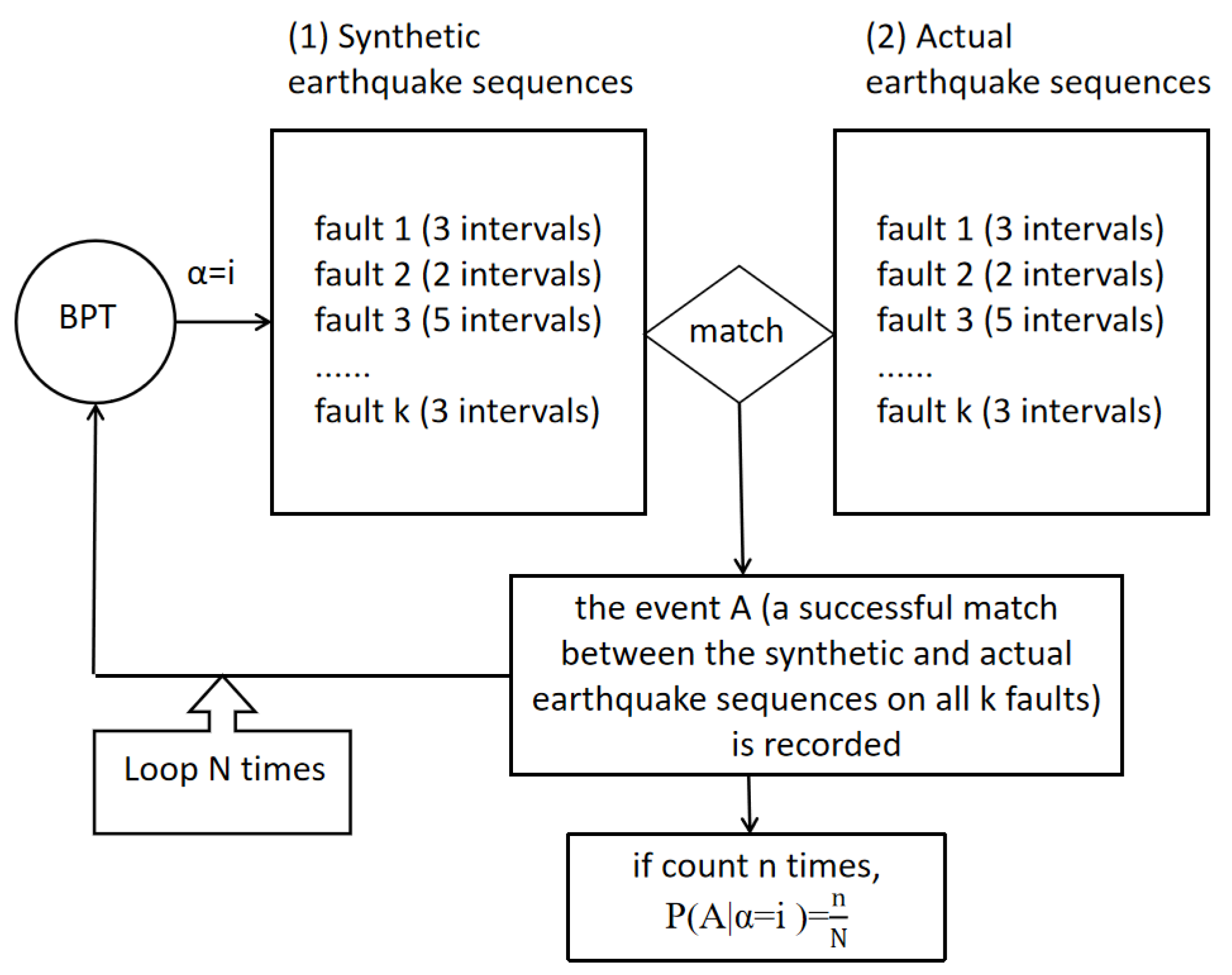
As illustrated in Figure 1, the method employed in this study is summarized as follows. The simulation is repeated N times, during which the event A (a successful match between the synthetic and actual earthquake sequences on all k faults) is recorded each time it occurs. The probability of event A for given values of α is denoted as:

$$\mathrm{P}\left(\mathrm{A}\right|\mathsf{\alpha }=\mathrm{i})={\displaystyle \frac{\mathrm{n}}{\mathrm{N}}}$$

(2)

where n is the number of successful matches. Thus, both the posterior distribution and the posterior mean value of the coefficient of variation α can be derived.

The method proposed in this paper is, in essence, based on the Bayesian principle (see Equation (3)).

$$\mathrm{P}({\mathrm{B}}_{\mathrm{i}}|\mathrm{A})={\displaystyle \frac{\mathrm{P}\left({\mathrm{B}}_{\mathrm{i}}\right)\mathrm{P}\left(\mathrm{A}\right|{\mathrm{B}}_{\mathrm{i}})}{\sum _{\mathrm{j}=1}^{\mathrm{n}}\mathrm{P}\left({\mathrm{B}}_{\mathrm{j}}\right)\mathrm{P}\left(\mathrm{A}\right|{\mathrm{B}}_{\mathrm{j}})}}$$

(3)

In Equation (3), $\mathrm{P}\left({\mathrm{B}}_{\mathrm{i}}\right)$ represents the prior probability. In the context of this study, $\mathrm{P}\left({\mathrm{B}}_{\mathrm{i}}\right)$ can be interpreted as $\mathrm{P}(\mathsf{\alpha }=\mathrm{i})$. The following assumption is adopted: according to Laplace’s principle, all possible values of α are assumed to be equally probable. That is, the prior distribution of $\mathsf{\alpha }$ is uniform over the interval [0, 1]. Under this assumption, $\mathrm{P}\left({\mathrm{B}}_{\mathrm{i}}\right)$ becomes a constant, and Equation (3) simplifies to:

$$\mathrm{P}({\mathrm{B}}_{\mathrm{i}}|\mathrm{A})={\displaystyle \frac{\mathrm{P}\left(\mathrm{A}\right|{\mathrm{B}}_{\mathrm{i}})}{\sum _{\mathrm{j}=1}^{\mathrm{n}}\mathrm{P}\left(\mathrm{A}\right|{\mathrm{B}}_{\mathrm{j}})}}$$

(4)

Within the framework of the BPT model, the parameter α can be configured to assume an equal probability distribution within the interval [0, 1]. When assigned the value α = 0, the model exhibits perfect periodicity; when α = 1, it corresponds to complete aperiodicity.

In this study, the event A in Equation (3) is defined as successful matching of k groups of synthetic datasets of ${\displaystyle \frac{\mathrm{T}}{{\mathrm{T}}_{\mathrm{a}\mathrm{v}\mathrm{e}}}}$ with k groups of actual datasets of ${\displaystyle \frac{\mathrm{T}}{{\mathrm{T}}_{\mathrm{a}\mathrm{v}\mathrm{e}}}}$ within a single simulation. For a given value of α, the frequency n of matching events across N Monte Carlo simulations is recorded. This enables the calculation of the probability of event A under different α values. The posterior probability $\mathrm{P}\left({\mathrm{B}}_{\mathrm{i}}\right|\mathrm{A})$, which represents the distribution of α-values, can then be computed using Equation (5).

$$\mathrm{P}(\mathrm{A}|{\mathrm{B}}_{\mathrm{i}})={\displaystyle \frac{\mathrm{n}}{\mathrm{N}}}$$

(5)

From both theoretical and practical perspectives, the posterior mean is the optimal choice for point estimation in Bayesian frameworks, especially for a seismic hazard assessment where uncertainty propagation is critical. This approach is particularly advantageous in paleoseismic studies, which typically involve limited sample sizes that can produce skewed or multimodal posterior distributions through Monte Carlo simulation. Unlike mode-based estimates that rely on single peak values and may be unreliable under such conditions, the posterior mean incorporates information from the entire distribution, providing more stable and theoretically robust parameter estimates. Consequently, this study employs the posterior mean as the α parameter in the BPT model.

2.2. Key Technologies

To implement the proposed method for estimating the coefficient of variation of recurrence intervals from paleoseismic sequences, several important aspects warrant further examination.

2.2.1. Model and Parameters

Various statistical distributions have been used to model the recurrence intervals of large earthquakes, including the lognormal, Weibull and gamma distributions, as well as the BPT model. In this study, the BPT model—widely adopted for its physical interpretability—is selected, although it is equally applicable to other models.

The BPT model is defined by two key parameters: μ, which is the average recurrence interval of large earthquakes on active faults, and α, which is the coefficient of variation of the recurrence interval. Once μ and α are specified, the probability density function (PDF) of the BPT model can be constructed and the synthetic recurrence interval data on the fault can then be randomly generated using the Monte Carlo method.

The methodology proposed in this paper involves the a matching technique that is designed to align the normalized recurrence interval datasets from synthetic and observed paleoseismic sequences. These ${\displaystyle \frac{\mathrm{T}}{{\mathrm{T}}_{\mathrm{a}\mathrm{v}\mathrm{e}}}}$ values are normalized independently of μ, meaning that the variability of the generated ${\displaystyle \frac{\mathrm{T}}{{\mathrm{T}}_{\mathrm{a}\mathrm{v}\mathrm{e}}}}$ data is unaffected by the value of μ in the BPT model. Therefore, while the implementation requires the specification of μ, it can be arbitrarily chosen without influencing the normalized distribution, as the matching process is based solely on the variability captured by α.

2.2.2. Matching Technique

The matching criteria between synthetic and observational data, which determine the requirements for reproducing real events, are crucial in Monte Carlo methods. Parsons’ (2008) Monte Carlo approach provides a framework for estimating recurrence interval distribution parameters in the presence of paleoseismic dating uncertainties. In this matching process, synthetic sequences are considered valid matches when exactly one earthquake occurs within each observational time window (defined by radiocarbon dating constraints) while no events occur in the intervals between windows.

However, this approach has inherent limitations: even when a synthetic earthquake falls within the temporal range of a paleoearthquake event, their temporal coincidence represents only a probabilistic match rather than a definitive correspondence. Specifically, larger uncertainties in paleoearthquake event dating ranges correspond to lower probabilities that any specific time point represents the true event occurrence. Consequently, paleoearthquake events with varying temporal uncertainties contribute unequally to statistical analysis, potentially introducing systematic bias in parameter estimation.

Furthermore, for paleoearthquake events with excessively narrow uncertainty windows, achieving matches becomes extremely difficult. In Parsons’ (2008) study involving four faults, even 10 million simulations failed to generate sufficient matched data for robust statistical analysis. The challenge is further compounded when earthquake sequences include precisely dated historical events.

The matching technique proposed in this study, while also employing Monte Carlo simulation, differs fundamentally from Parsons’ approach in three key aspects:

(1). Multi-fault simultaneous matching: Rather than focusing on individual faults, our Monte Carlo method simultaneously matches data across multiple faults. A reproduction event is recorded only when synthetic datasets match observational datasets on all k faults simultaneously within a single simulation.

(2). Recurrence interval matching instead of event matching: Instead of matching individual earthquake events, our method matches recurrence interval datasets. For instance, if one fault has three actual recurrence intervals, a single simulation generates three corresponding synthetic recurrence intervals. After normalization, these are compared pairwise in ascending order, and a fault achieves a match when all differences fall within the predefined threshold. A reproduction event is recorded only when all k faults achieve simultaneous matching in a single simulation.

(3). Modified matching criteria: While Parsons’ method requires exactly one earthquake per observational time window with no events between windows, our approach defines a match when the absolute difference between normalized recurrence intervals (${\displaystyle \frac{\mathrm{T}}{{\mathrm{T}}_{\mathrm{a}\mathrm{v}\mathrm{e}}}}$) falls within 0.05. This approach treats all paleoearthquake events with equal weight, thereby minimizing bias introduced by dating uncertainties. It also circumvents the limitations of Parsons’ method, where certain earthquake sequences with extremely precise age constraints or well-documented historical events cannot achieve reproduction regardless of simulation count.

(4). The selection of the matching threshold is critical. The matching precision must be neither overly strict nor too lenient. Excessively high precision may require impractically large numbers of simulations to achieve matches, while overly low precision may yield high match rates but poor representation of actual recurrence behavior. Therefore, this study defines a match when the absolute difference between synthetic and actual (${\displaystyle \frac{\mathrm{T}}{{\mathrm{T}}_{\mathrm{a}\mathrm{v}\mathrm{e}}}}$) values falls within 0.05. Through a validation experiment, we determined that coefficient of variation values remain stable and consistent when matching thresholds are set between 0.01 and 0.1. Consequently, we selected a matching threshold of 0.05.

2.2.3. Algorithm Optimization

When the database contains a limited number of faults and their corresponding seismic sequences, the Monte Carlo method can be utilized directly to randomly generate k synthetic sequences that correspond to the observed sequences from k faults. However, when the database includes a large number of faults, achieving simultaneous matching across multiple faults requires a substantial number of simulations. The methodology employed in this study estimates the distribution of the coefficient of variation by calculating the frequency of matches. However, obtaining stable and reliable statistical results becomes difficult if the number of successful matches is too low.

Assuming that earthquakes on different faults occur independently, the probability of achieving a match with each individual fault—ranging from the first to the kth fault—can be denoted as ${\mathrm{P}}_1$,${\mathrm{P}}_2$,${\mathrm{P}}_3$…${\mathrm{P}}_{\mathrm{k}}$. Under this assumption, the probability of simultaneously matching all k faults in a single simulation can be calculated using Equation (6).

$${\mathrm{P}=\mathrm{P}}_1{\mathrm{P}}_2{\mathrm{P}}_3\dots {\mathrm{P}}_{\mathrm{k}}$$

(6)

2.2.4. Paleoseismic Database

Due to the limited number of recurrence intervals, it is difficult to obtain reliable results from the data of a single fault. This limitation introduces significant uncertainty in the estimation of the coefficient of variation when conducting statistical analysis. Although the uncertainty is reduced when estimating a generic coefficient of variation using paleoseismic sequences from multiple faults, it remains challenging to accurately capture the effects of varying tectonic settings and earthquake magnitudes.

Accordingly, this study restricts the paleoseismic database to faults located within specific seismotectonic zones. This targeted approach enables the creation of databases that reflect how distinct tectonic environments influence the coefficient of variation across different geographical regions.

The selection of paleoseismic data in this study follows these criteria:

(1). Events lacking either upper or lower bounds of paleoseismic dating are excluded;

(2). Fault data from the Late Pleistocene period are prioritized, as older data are more likely to be incomplete;

(3). Preference is given to the most recently published paleoseismic surveys;

(4). In cases of graded ruptures, full rupture events must not be included in the same sequence as secondary rupture events.

2.2.5. Uncertainty in Paleoseismic Dating

Statistical analysis of paleoseismic data faces a fundamental challenge: the inherent uncertainty in dating paleoseismic events. Geological investigations typically constrain events within temporal windows rather than providing precise occurrence times, substantially complicating the determination of accurate recurrence intervals. To address this limitation, Ellsworth et al. [7] developed a bootstrap resampling procedure applied to probability density functions derived from radiocarbon dating, subsequently employing maximum likelihood estimation to determine Brownian Passage Time (BPT) model parameters for recurrence intervals and coefficients of variation.

Parsons’ Monte Carlo method estimates parameters of recurrence interval distributions while incorporating uncertainties from paleoseismic age-dating techniques [12]. This approach compiles synthetic earthquake sequences satisfying two criteria: (1) exactly one seismic event occurs within each observed window (time intervals constrained by radiocarbon dating), and (2) no events occur between these windows. Any earthquake occurring within a defined window is considered a validated event. Thus, while Parsons’ method utilizes dating uncertainties for event matching during sequence generation, it does not propagate these uncertainties into the final parameter estimation process.

Nevertheless, a fundamental limitation persists in this matching framework: even when synthetic earthquakes fall within paleoseismic event windows, the probability of actual temporal coincidence remains finite and inversely related to dating uncertainty magnitude. Consequently, events with heterogeneous dating uncertainties contribute unequally to statistical analyses, potentially introducing systematic bias.

The present study addresses this limitation through a novel matching algorithm that compares normalized recurrence interval datasets between synthetic and paleoseismic sequences. Matches are established when rank-ordered dataset differences fall within a 0.05 threshold, ensuring equal weighting of all paleoseismic events regardless of individual dating uncertainties, thereby minimizing uncertainty-related bias.

Two computational scenarios are implemented: (1) when dating uncertainty is neglected, median values of temporal windows are directly substituted in simulations; (2) when uncertainty is incorporated, values are randomly sampled from uniform distributions within each event’s temporal window for every simulation iteration. This framework enables comprehensive uncertainty propagation through extensive Monte Carlo simulation ensembles, where each realization represents a distinct paleoseismic sequence configuration. Historical earthquakes maintain fixed occurrence times across all simulations, while paleoseismic events are characterized by uniformly distributed random occurrence times within their respective uncertainty windows.

3. Calculation Examples

To effectively demonstrate the proposed method for estimating the coefficient of variation (α) of recurrence intervals for large earthquakes, both a smaller and a larger region were selected for example calculations. The smaller region is the Western Qilian Mountain–Hexi Corridor, an area characterized by numerous active faults with strong Holocene activities and a well-established research foundation. The available data from this region generally satisfy the sample size requirements for statistical analysis. The broader region selected is western China. Notably, there are significant differences in tectonic environments and seismicity between eastern and western China. These contrasts make each region suitable for studying the spatial variation of recurrence behavior, particularly for comparative analysis between eastern and western China.

This study aims to develop a parameter estimation method for the coefficient of variation α, with computational examples that aggregate different paleoseismic sequences within a region to derive a universal α value representing a regional average. However, this averaging process may obscure underlying physical relationships. Studies have demonstrated that the coefficient of variation α in the Brownian Passage Time (BPT) model exhibits systematic variations across different fault systems. Faults with high slip rates and those hosting large characteristic earthquakes typically display lower α values (0.3–0.5), reflecting more regular recurrence patterns. Moreover, different fault types exhibit distinct α value distributions [7,8,13,14,15,16,17,18]. However, due to limitations in paleoseismic data, multi-factor coupling effects, and regional tectonic variations, specific correlation patterns remain controversial. Establishing reliable quantitative relationships requires additional high-quality data and refined statistical analyses, which are crucial for avoiding the potential masking of true fault recurrence characteristics that may result from simple regional averaging of α values.

Therefore, the illustrative calculations presented in this study have certain limitations, and obtaining more scientifically robust and accurate results requires further classified investigations. This research represents only a preliminary exploration of a novel statistical method for coefficient of variation α estimation. The computational results should be considered as reference values only, and practical applications would require more comprehensive high-quality datasets and sophisticated statistical analyses.

3.1. Example 1: Western Qilian Mountains-Hexi Corridor

The Qilian Mountains–Hexi Corridor is located in northwestern China. The Qilian Mountains–Hexi Corridor is located approximately between 93° E–104° E and 37° N–40° N. It belongs to the Qilian Orogenic Belt, which is an important component of the Central Orogenic System, situated between the Alxa Block and Qaidam Block. The region is characterized by NW-SE trending linear structural patterns, with the Qilian Mountains dominated by thrust-nappe structures and the Hexi Corridor consisting of multiple fault-controlled basins. This area serves as a crucial transitional zone connecting the stable North China Craton with the active Tibetan Plateau tectonic system, representing the northern boundary of the remote effects from the India–Eurasia continental collision [19].

The primary active faults within the western tectonic zone of this region are predominantly reverse faults, which exhibit relatively strong seismic activity. Years of research have shown that these reverse faults contain some of the most recent and well-documented paleoseismic data in China [19,20,21,22,23,24,25]. Additionally, the region is rich in historical earthquake records, fulfilling the fundamental requirements for recurrence interval modeling.

The selected faults include the Yumen–Beidahe fault, the Jintananshan fault, the northern rim fault of Yumu Mountain, the eastern rim fault of Yumu Mountain, the Sunan fault, and the Fodongmiao–Hongyazi fault. The paleoseismic and historical earthquake records from these fault systems collectively constitute the primary database for determining the coefficient of variation (α) of earthquake recurrence intervals, as summarized in

Table 1. Database consisting of seven earthquake sequences in western Qilian Mountains–Hexi Corridor in China.

No.	Fault Name	Number of Paleoearthquakes	Age of Paleoseismic Events (Years BP)	Number of Recurrence Intervals	Source of Paleoseismic Data
1	Northern Margin of Yumu mountain Fault	3	E1: >10,500 ± 600 E2: 7850 ± 650 E3: 3800 ± 100 A.D. 180	2	[20]
2	Liyuanhekou–Heihekou Segment of Eastern Margin of Yumu mountain Fault	5	E1: 15,700 E2: 13,150 ± 150 E3: 10,500 E4: 8750 ± 250 E5: 5000	4	[19]
3	Linze Segment of Eastern Margin of Yumu Mountain Fault	4	E1: 8895 ± 125 E2: 6718 ± 39 E3: 4960 ± 27 E4: 2438 ± 40	3	[19]
4	Fodongmiao–Hongyazi Fault	4	E1: 10,600 ± 900 E2: 7100 ± 100 E3: 3370 ± 30 A.D. 1609	3	[21]
5	West Segment of the Jintananshan North-margin Fault	4	E1: 15,160 ± 1290 E2: 9900 ± 500 E3: 6000 E4: 3500 ± 400	3	[22]
6	Yumen–Beidahe Fault	3	E1: 9415 ± 1115 E2: 4590 ± 790 E3: 1785 ± 145 E4: <1630 ± 170	2	[23,24]
7	Sunan Fault	3	E1: 2200 E2: 1680 E3: 700	2	[25]

.

It should be noted that in this study, paleoseismic events lacking either upper or lower absolute dating constraints are excluded from subsequent calculations. These events are not used for recurrence interval calculations or included in further statistical analyses. For example, event E1 of the Northern Margin of Yumu Mountain Fault and event E4 of the Yumen–Beidahe Fault are listed in Table 1.

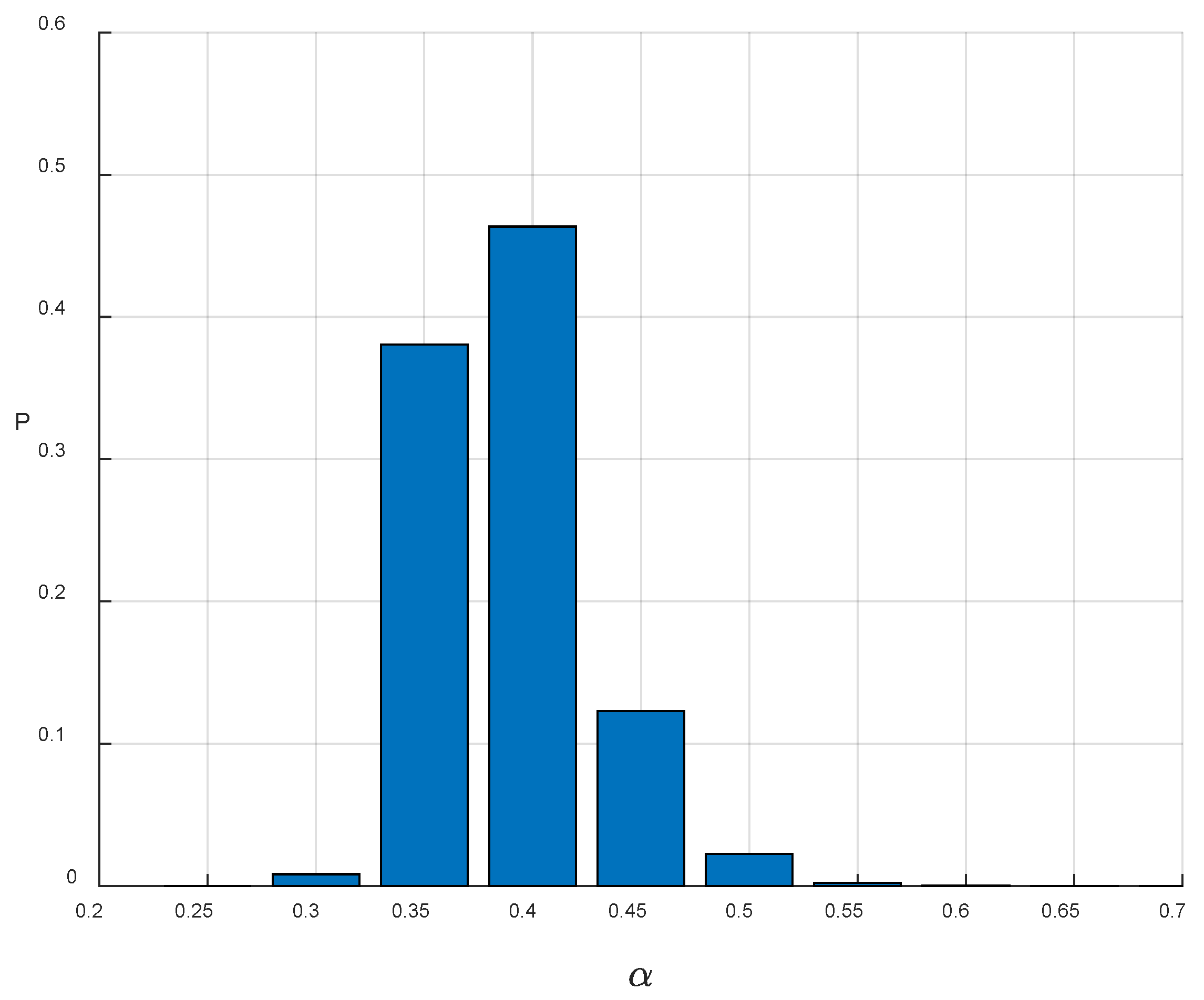
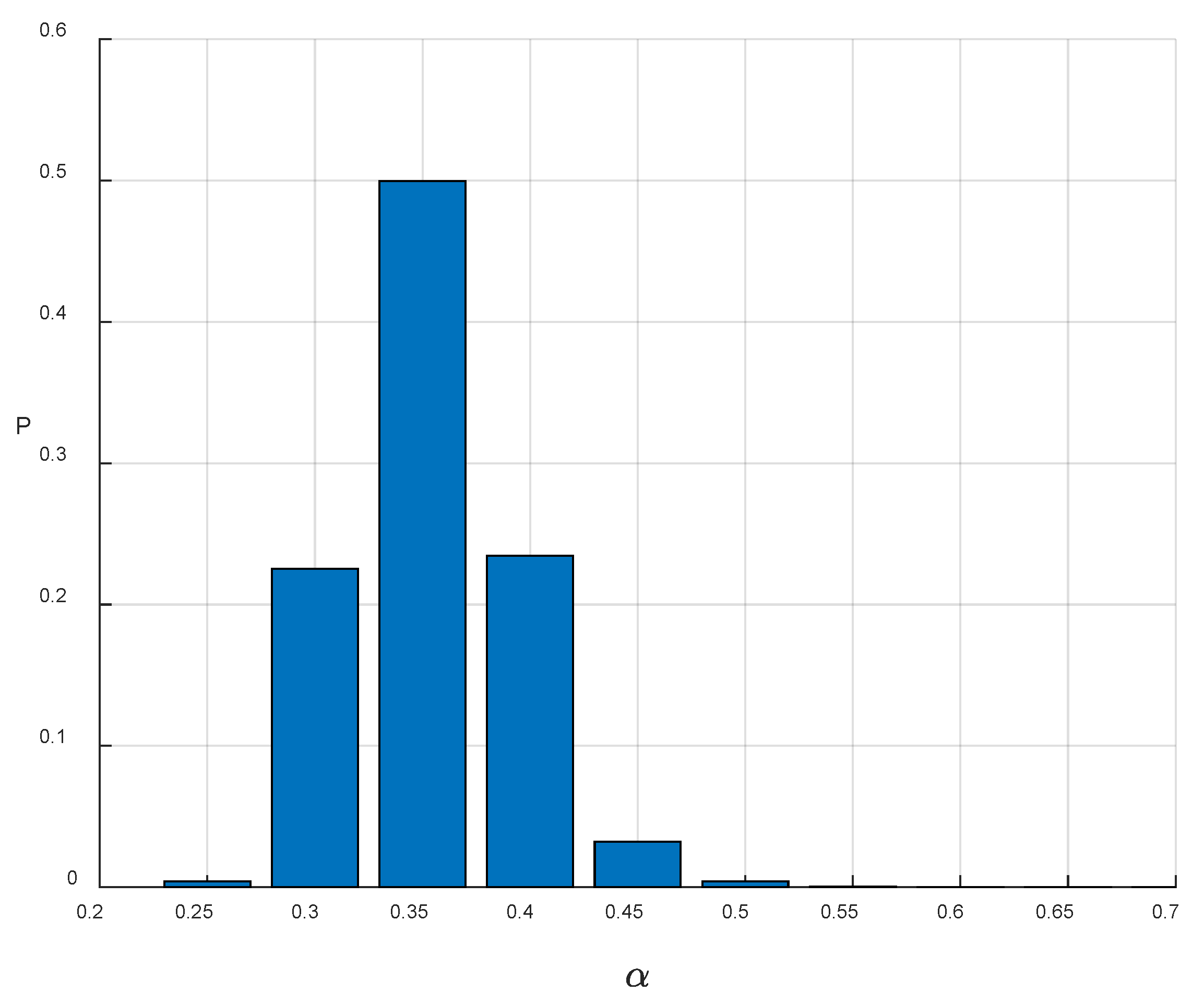
Using the proposed method for estimating the coefficient of variation (α), a total of 1,000,000 Monte Carlo simulations were conducted for the Western Qilian Mountains–Hexi Corridor region. Figure 2 presents the results obtained without accounting for paleoseismic dating uncertainty, while Figure 3 displays the results with this uncertainty incorporated. The findings indicate that the impact of considering paleoseismic dating uncertainty is minimal. When dating uncertainty is not considered, the posterior mean of α is 0.36. When dating uncertainty is incorporated, the corresponding values slightly decrease to 0.34. This small difference suggests that, in this case, dating uncertainty has a limited influence on the estimated coefficient of variation.

For comparative purposes, this study also conducts a Monte Carlo simulation based exclusively on the paleoseismic sequence from the western segment of the Jinta Nanshan north-margin fault. This simulation yields the distribution of the coefficient of variation (α) for recurrence intervals, as illustrated in Figure 4.

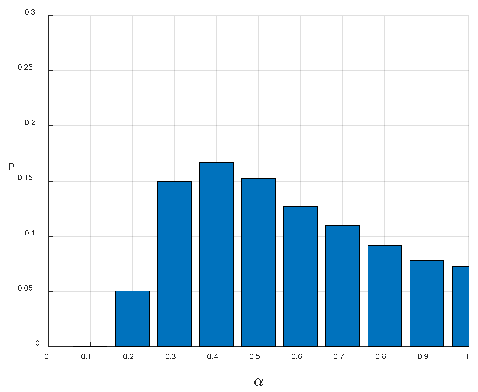
The computational results reveal that when only a single fault is used, the estimated coefficient of variation exhibits significantly greater uncertainty. In this case, the posterior mean of α is 0.57. As shown in Figure 4, the probability of obtaining a larger α is substantially higher than that observed in Figure 3.

This result can be explained from a statistical perspective. When the number of constraints is limited—such as when only one paleoseismic sequence is available—a higher α can more readily match the actual sequence. Conversely, as the number of constraints increases through the inclusion of multiple fault sequences, the likelihood of a large α producing a match decreases accordingly.

3.2. Example 2: Western China

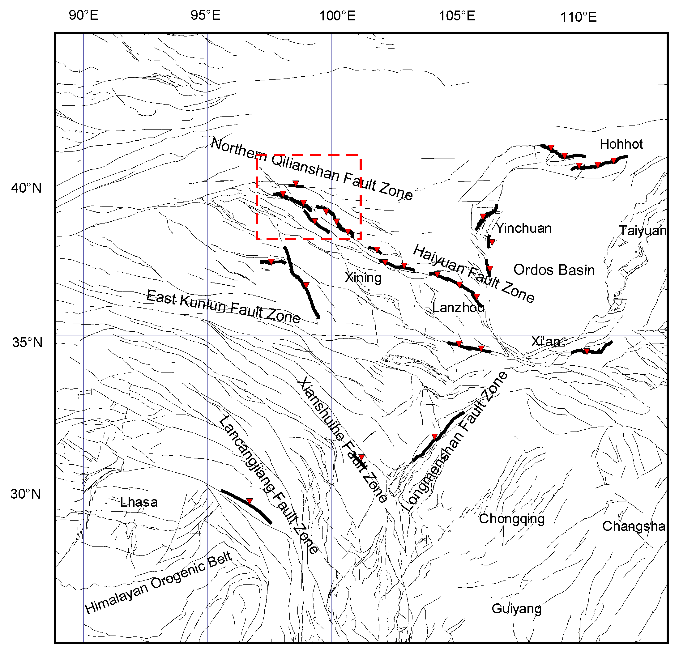
To explore the applicability of the proposed method on a broader spatial scale, this study selects western China as the target region (Figure 5). A database comprising paleoseismic sequences from 29 representative faults in western China has been established, as detailed in Table 2.

Significant differences exist between eastern and western China regarding geological structure and seismic activity patterns. The eastern region is predominantly characterized by the Sino-Korean Paraplatform and Yangtze Paraplatform, exhibiting relatively stable tectonic conditions with seismic activity dominated by shallow to intermediate-depth earthquakes that, despite their moderate magnitudes, pose considerable risks to densely populated areas. In contrast, the western region is mainly composed of young orogenic belts including the Tibetan Plateau, Tianshan Mountains, and Kunlun Mountains, where intense tectonic activity occurs, making it one of the most seismically active regions globally, frequently generating large and great earthquakes with deeper hypocenters and higher magnitudes. The boundary between these two regions primarily follows the Daxing’anling–Taihang–Wushan–Xuefeng tectonic belt, which serves not only as a crucial geological structural boundary but also as a fundamental demarcation line distinguishing the seismic activity intensity between eastern and western China [26,27].

The 29 faults examined in this research are mainly located across the dynamic structural regions of the Tibetan Plateau and its surrounding areas, encompassing the Longmenshan Fault Zone, Haiyiuan Fault Zone, Xianshuihe Fault Zone, and others. These fault structures demonstrate uniformity in their large-scale geological framework, representing significant active fault systems developed under continental convergence conditions.

Table 2. Database consisting of 29 earthquake sequences in western China.

No.	Fault Name	Fault Types	Number of Paleoearthquakes	Age of Paleoseismic Events (Years BP)	Number of Recurrence Intervals	Source of Paleoseismic Data
1	Maomaoshan–Jinqianghe Fault, Eastern North Qilian Mountains	Left-lateral strike–slip fault	5	E1: 9000 ± 300 E2: 6600 ± 300 E3: 5000 ± 300 E4: 3700 ± 300 E5: 1800 ± 300	4	[28]
2	Mid-segment rupture of Haiyuan Fault	Left-lateral strike–slip fault	7	E1: 6595 ± 275 E2: 5770 ± 200 E3: 4965 ± 925 E4: 3382 ± 589 E5: 2765 ± 355 E6: 2240 ± 450 E7: 1275 ± 350	6	[29,30]
3	Rupture of Western Haiyuan Fault	Left-lateral strike–slip fault	4	E1: 6595 ± 275 E2: 4680 ± 430 E3: 2655 ± 225 E4: 1005 ± 465	3	[29,30]
4	Rupture of Whole Haiyuan Fault	Left-lateral strike–slip fault	3	E1: 10,770 ± 1125 E2: 6595 ± 275 E3: A.D. 1920	2	[29,30]
5	Hohhot section of Daqingshan Piedmont Fault	Thrust fault	5	E1: ≤18,800 E2: 16,965 ± 955 E3: 14,600 ± 710 E4: 11,820 ± 690 E5: 9465 ± 255 E6: 6830 ± 260 E7: ≥4030	4	[31]
6	Tuyouqi Section of Daqingshan Piedmont Fault	Thrust fault	5	E1: 10,309 ± 991 E2: 8760 ± 500 E3: 4545 ± 466 E4: 3650 ± 280 A.D. 849	4	[31]
7	Tuzuoqi Section of Daqingshan Piedmont Fault	Thrust fault	3	E1: >10,790 E2: 8276 ± 577 E3: 6396 ± 891 E4: 1947 ± 67	2	[31]
8	Lingwu Fault	Thrust fault	5	E1: 27,150 ± 778 E2: 20,000 E3: 13,070 ± 60 E4: 10,586 ± 50 E5: 6000	4	[32]
9	Daofu Section of Xianshuihe Fault	Left-lateral strike–slip fault	3	A.D. 1792 A.D. 1904 A.D. 1981	2	[33]
10	Eastern Piedmont Fault of the Luoshan Mountain	Thrust fault	4	E1: 8200 ± 600 E2: 5020 ± 70 E3: 3331 ± 92 A.D. 1561	3	[34]
11	Eastern Piedmont Fault of the Helanshan Mountain	Thrust fault	5	E1: 8240 ± 170 E2: 6330 ± 80 E3: 4760 ± 80 E4: 2675 ± 70 A.D. 1739	4	[34]
12	Large Shetai Section of the Seerten Piedmont Fault	Thrust fault	4	E1: 31,690 ± 1770 E2: 23,000 ± 1320 E3: 15,420 ± 870 E4: 7440 ± 440	3	[35]
13	Wulanhudong Segment of the Seerten Piedmont Fault	Thrust fault	4	E1: 25,130 ± 1430 E2: 14,570 ± 820 E3: 11,660 ± 650 E4: 7220 ± 400	3	[35]
14	Lenglongling Fault	Left-lateral strike–slip fault	5	E1: 5926 E2: 4050 ± 160 E3: 2900 ± 270 E4: 1560 ± 360 A.D. 1540	4	[36]
15	Elashan Fault	Left-lateral strike–slip fault	5	E1: 12,500 ± 100 E2: 10,000 ± 150 E3: 6000 ± 100 E4: 4100 ± 300 E5: 2600 ± 400	4	[37]
16	Huashan Piedmont Fault	Thrust fault	5	E1: 7500 E2: 5610 E3: 4250 E4: 2750 ± 250 A.D. 1559	4	[38]
17	Northern Margin of Yumu Mountain Fault	Thrust fault	3	E1: >10,500 ± 600 E2: 7850 ± 650 E3: 3800 ± 100 A.D. 180	2	[20]
18	Liyuanhekou–Heihekou Segment of Eastern Margin of Yumu Mountain Fault	Thrust fault	5	E1: 15,700 E2: 13,150 ± 150 E3: 10,500 E4: 8750 ± 250 E5: 5000	4	[19]
19	Linze Segment of Eastern Margin of Yumu Mountain Fault	Thrust fault	4	E1: 8895 ± 125 E2: 6718 ± 39 E3: 4960 ± 27 E4: 2438 ± 40	3	[19]
20	Huancheng–Shuangta Fault	Thrust fault	4	E1: 15,930 ± 1160 E2: 9460 ± 700 E3: 5000 ± 500 A.D. 1927	3	[39]
21	Yuanfeng Fault Section of North Margin of West Qinling	Thrust fault	4	E1: 12,500 ± 500 E2: 7500 ± 500 E3: 5000 A.D. 1276	3	[40,41]
22	Guomatan Fault Section of North Margin of West Qinling	Thrust fault	3	E1: 12,450 E2: 5480 ± 60 A.D. 1936	2	[40,41]
23	Sunan Fault	Thrust fault	3	E1: 2200 E2: 1680 E3: 700	2	[25]
24	North Margin Fault of Bayingol River	Thrust fault	3	E1: 32,700 ± 1450 E2: 15,540 ± 1320 E3: 3245 ± 330	2	[42]
25	Beichuan–Yingxiu Fault	Thrust fault	3	E1: 5825 ± 95 E2: 2800 ± 500 A.D. 2008	2	[43]
26	Southeast Segment of Jali–Chayu Fault	Left-lateral strike–slip fault	5	E1: 15,895 ± 235 E2: 1160 ± 940 E3: 9095 ± 465 E4: 2470 ± 310 E5: 650	4	[44]
27	Fodongmiao–Hongyazi Fault	Thrust fault	4	E1: 10,600 ± 900 E2: 7100 ± 100 E3: 3370 ± 30 A.D. 1609	3	[21]
28	West Segment of the Jintananshan North-margin Fault	Thrust fault	4	E1: 15,160 ± 1290 E2: 9900 ± 500 E3: 6000 E4: 3500 ± 400	3	[22]
29	Yumen–Beidahe Fault	Left-lateral strike–slip fault	3	E1: 9415 ± 1115 E2: 4590 ± 790 E3: 1785 ± 145 E4: <1630 ± 170	2	[23,24]

Table 2. Database consisting of 29 earthquake sequences in western China.

No.	Fault Name	Fault Types	Number of Paleoearthquakes	Age of Paleoseismic Events (Years BP)	Number of Recurrence Intervals	Source of Paleoseismic Data
1	Maomaoshan–Jinqianghe Fault, Eastern North Qilian Mountains	Left-lateral strike–slip fault	5	E1: 9000 ± 300 E2: 6600 ± 300 E3: 5000 ± 300 E4: 3700 ± 300 E5: 1800 ± 300	4	[28]
2	Mid-segment rupture of Haiyuan Fault	Left-lateral strike–slip fault	7	E1: 6595 ± 275 E2: 5770 ± 200 E3: 4965 ± 925 E4: 3382 ± 589 E5: 2765 ± 355 E6: 2240 ± 450 E7: 1275 ± 350	6	[29,30]
3	Rupture of Western Haiyuan Fault	Left-lateral strike–slip fault	4	E1: 6595 ± 275 E2: 4680 ± 430 E3: 2655 ± 225 E4: 1005 ± 465	3	[29,30]
4	Rupture of Whole Haiyuan Fault	Left-lateral strike–slip fault	3	E1: 10,770 ± 1125 E2: 6595 ± 275 E3: A.D. 1920	2	[29,30]
5	Hohhot section of Daqingshan Piedmont Fault	Thrust fault	5	E1: ≤18,800 E2: 16,965 ± 955 E3: 14,600 ± 710 E4: 11,820 ± 690 E5: 9465 ± 255 E6: 6830 ± 260 E7: ≥4030	4	[31]
6	Tuyouqi Section of Daqingshan Piedmont Fault	Thrust fault	5	E1: 10,309 ± 991 E2: 8760 ± 500 E3: 4545 ± 466 E4: 3650 ± 280 A.D. 849	4	[31]
7	Tuzuoqi Section of Daqingshan Piedmont Fault	Thrust fault	3	E1: >10,790 E2: 8276 ± 577 E3: 6396 ± 891 E4: 1947 ± 67	2	[31]
8	Lingwu Fault	Thrust fault	5	E1: 27,150 ± 778 E2: 20,000 E3: 13,070 ± 60 E4: 10,586 ± 50 E5: 6000	4	[32]
9	Daofu Section of Xianshuihe Fault	Left-lateral strike–slip fault	3	A.D. 1792 A.D. 1904 A.D. 1981	2	[33]
10	Eastern Piedmont Fault of the Luoshan Mountain	Thrust fault	4	E1: 8200 ± 600 E2: 5020 ± 70 E3: 3331 ± 92 A.D. 1561	3	[34]
11	Eastern Piedmont Fault of the Helanshan Mountain	Thrust fault	5	E1: 8240 ± 170 E2: 6330 ± 80 E3: 4760 ± 80 E4: 2675 ± 70 A.D. 1739	4	[34]
12	Large Shetai Section of the Seerten Piedmont Fault	Thrust fault	4	E1: 31,690 ± 1770 E2: 23,000 ± 1320 E3: 15,420 ± 870 E4: 7440 ± 440	3	[35]
13	Wulanhudong Segment of the Seerten Piedmont Fault	Thrust fault	4	E1: 25,130 ± 1430 E2: 14,570 ± 820 E3: 11,660 ± 650 E4: 7220 ± 400	3	[35]
14	Lenglongling Fault	Left-lateral strike–slip fault	5	E1: 5926 E2: 4050 ± 160 E3: 2900 ± 270 E4: 1560 ± 360 A.D. 1540	4	[36]
15	Elashan Fault	Left-lateral strike–slip fault	5	E1: 12,500 ± 100 E2: 10,000 ± 150 E3: 6000 ± 100 E4: 4100 ± 300 E5: 2600 ± 400	4	[37]
16	Huashan Piedmont Fault	Thrust fault	5	E1: 7500 E2: 5610 E3: 4250 E4: 2750 ± 250 A.D. 1559	4	[38]
17	Northern Margin of Yumu Mountain Fault	Thrust fault	3	E1: >10,500 ± 600 E2: 7850 ± 650 E3: 3800 ± 100 A.D. 180	2	[20]
18	Liyuanhekou–Heihekou Segment of Eastern Margin of Yumu Mountain Fault	Thrust fault	5	E1: 15,700 E2: 13,150 ± 150 E3: 10,500 E4: 8750 ± 250 E5: 5000	4	[19]
19	Linze Segment of Eastern Margin of Yumu Mountain Fault	Thrust fault	4	E1: 8895 ± 125 E2: 6718 ± 39 E3: 4960 ± 27 E4: 2438 ± 40	3	[19]
20	Huancheng–Shuangta Fault	Thrust fault	4	E1: 15,930 ± 1160 E2: 9460 ± 700 E3: 5000 ± 500 A.D. 1927	3	[39]
21	Yuanfeng Fault Section of North Margin of West Qinling	Thrust fault	4	E1: 12,500 ± 500 E2: 7500 ± 500 E3: 5000 A.D. 1276	3	[40,41]
22	Guomatan Fault Section of North Margin of West Qinling	Thrust fault	3	E1: 12,450 E2: 5480 ± 60 A.D. 1936	2	[40,41]
23	Sunan Fault	Thrust fault	3	E1: 2200 E2: 1680 E3: 700	2	[25]
24	North Margin Fault of Bayingol River	Thrust fault	3	E1: 32,700 ± 1450 E2: 15,540 ± 1320 E3: 3245 ± 330	2	[42]
25	Beichuan–Yingxiu Fault	Thrust fault	3	E1: 5825 ± 95 E2: 2800 ± 500 A.D. 2008	2	[43]
26	Southeast Segment of Jali–Chayu Fault	Left-lateral strike–slip fault	5	E1: 15,895 ± 235 E2: 1160 ± 940 E3: 9095 ± 465 E4: 2470 ± 310 E5: 650	4	[44]
27	Fodongmiao–Hongyazi Fault	Thrust fault	4	E1: 10,600 ± 900 E2: 7100 ± 100 E3: 3370 ± 30 A.D. 1609	3	[21]
28	West Segment of the Jintananshan North-margin Fault	Thrust fault	4	E1: 15,160 ± 1290 E2: 9900 ± 500 E3: 6000 E4: 3500 ± 400	3	[22]
29	Yumen–Beidahe Fault	Left-lateral strike–slip fault	3	E1: 9415 ± 1115 E2: 4590 ± 790 E3: 1785 ± 145 E4: <1630 ± 170	2	[23,24]

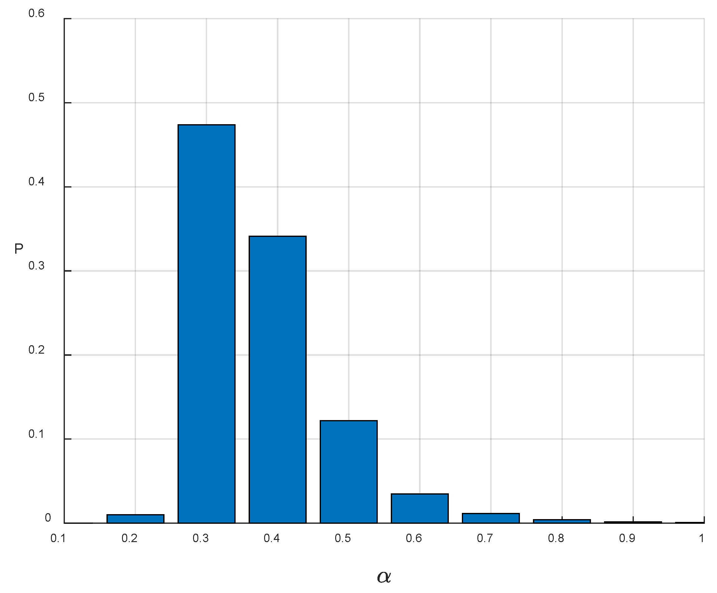
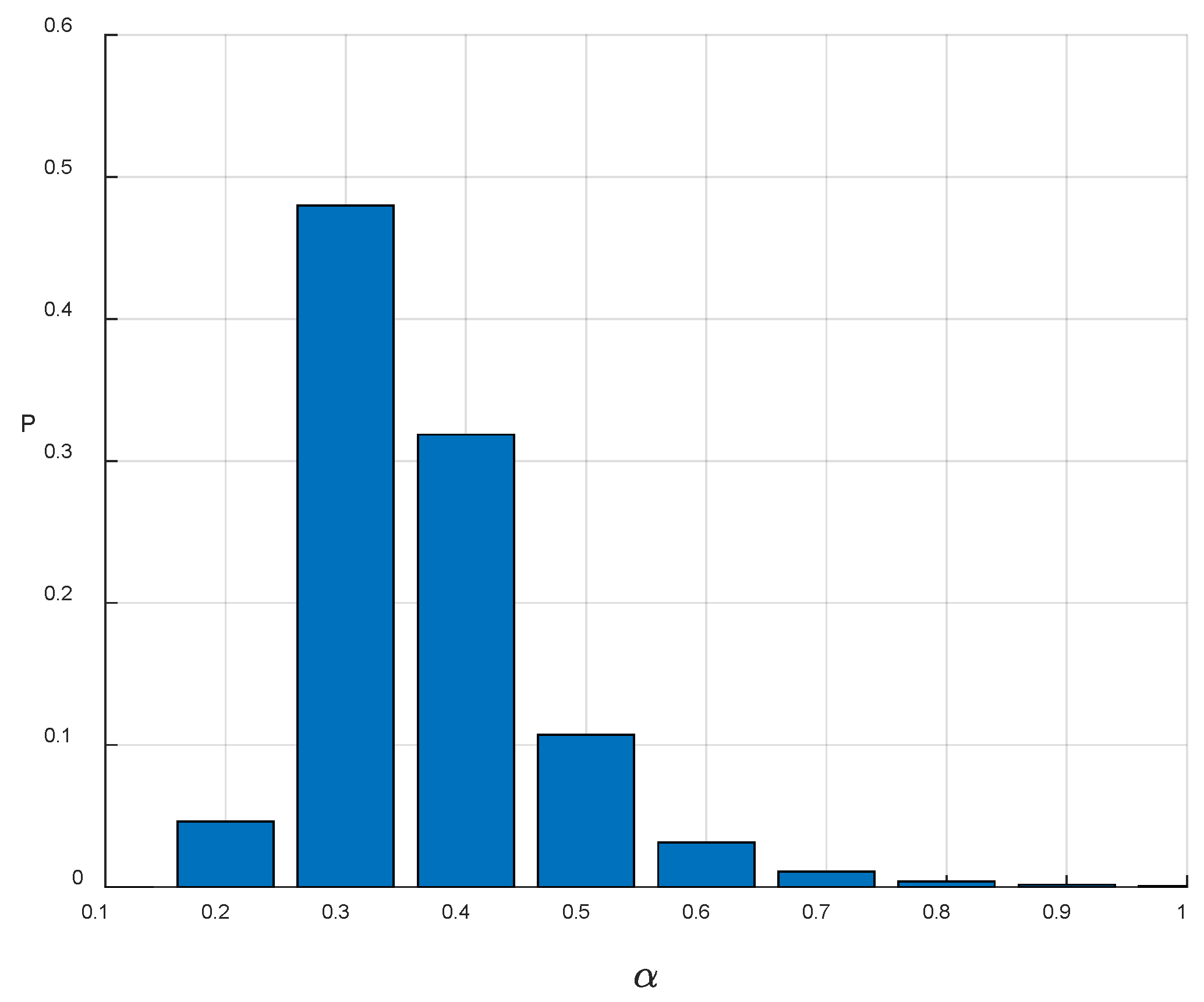
Using the proposed method for estimating the coefficient of variation, a total of 1,000,000 Monte Carlo simulations were conducted to evaluate the recurrence interval coefficient of variation in western China. Figure 6 presents the results obtained without accounting for paleoseismic dating uncertainty, while Figure 7 displays the results with this uncertainty incorporated.

The findings indicate slight differences between the two sets of calculations. When dating uncertainty is not considered, the posterior mean of α is 0.39. In contrast, when dating uncertainty is incorporated, the value decreases to 0.36. This result suggests that accounting for dating uncertainty can have a measurable effect on the estimated coefficient of variation.

Moreover, as the target area expands and the number of faults and paleoseismic sequences increases, the distribution of recurrence interval coefficients of variation (α) in western China—as shown in Figure 6 and Figure 7—exhibits reduced uncertainty. Additionally, the probability of larger α values occurring is lower compared to the distribution observed in the Western Qilian Mountains–Hexi Corridor, as presented in Figure 3 and Figure 4.

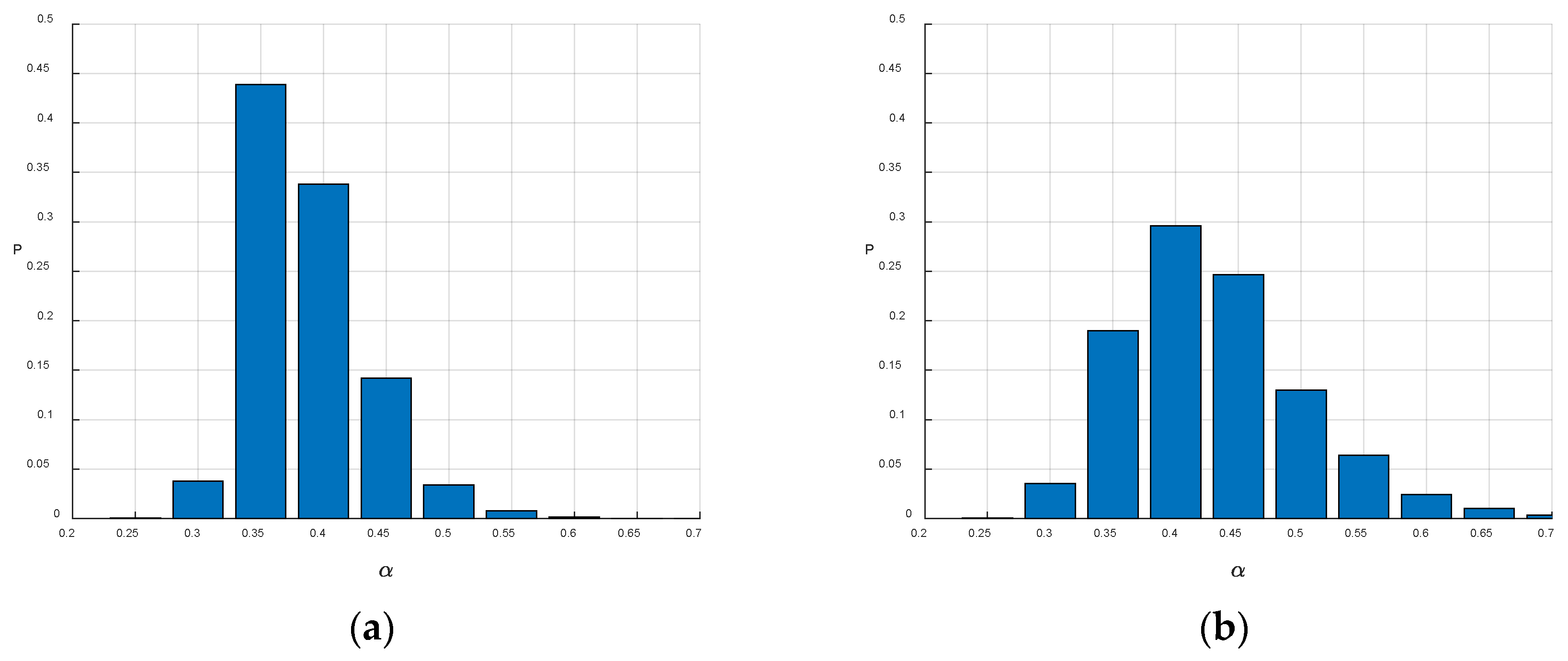
Considering the influence of multiple factors on the coefficient of variation, for regions with abundant paleoseismic data, we can also conduct classification-based statistics according to fault types. To demonstrate the application of our proposed method in further classification-based analysis, we have supplemented our study with an additional classification statistical example. Based on the fault type data in Table 1, we separately applied our method to calculate the coefficients of variation for strike–slip and thrust faults, which comprise 20 thrust faults and 9 strike–slip faults, respectively (see Figure 8). Without considering the uncertainties in paleoseismic age determination, the coefficient of variation α derived from strike–slip faults is 0.45, while that obtained from thrust faults is 0.37, indicating a measurable difference between the two fault types. Nevertheless, in light of the existing uncertainties, this finding should be treated as tentative and warrants further verification in diverse regional and fault system contexts. Relative to Figure 6, smaller sample sizes increase uncertainty and also raise the probability of larger coefficient of variation α values.

There may be numerous fault parameters related to the coefficient of variation. The purpose of this calculation example is to preliminarily explore the application of the parameter estimation method proposed in this paper for further classification-based statistics, employing only a simple classification based on fault types. Therefore, the statistical method still has certain limitations, and the results are provided for reference only.

4. Discussion

This paper proposes a novel methodology for estimating the recurrence interval coefficient of variation (α) from paleoseismic sequences. The method utilizes paleoseismic data from multiple faults within a given study region to derive a generalized coefficient of variation (α) for Brownian Passage Time (BPT) distribution.

Obtaining reliable statistical results from individual faults is challenging due to the limited number of available recurrence intervals. This limitation introduces considerable uncertainty in estimating the coefficient of variation for recurrence intervals. Although deriving a generic coefficient of variation (α) based on paleoseismic sequences across multiple faults helps reduce this uncertainty, it remains difficult to accurately capture the influence of varying tectonic settings on α. Therefore, the implementation of the proposed method assumes that the recurrence of large earthquakes on multiple faults within a specific tectonic environment exhibits consistent variability. However, this does not restrict the method’s application to this single assumption. The proposed approach can accommodate more refined statistical criteria; for instance, this study further classifies faults by type for statistical analysis in western China. The assumption that faults within a specific tectonic environment share similar variability represents a relatively broad and lenient classification that does not consider correlations between other fault characteristics and the coefficient of variation α. Consequently, when paleoseismic data are sufficiently abundant, the proposed method can be applied with more refined classification schemes for statistical analysis of the coefficient of variation.

The case study presented in this research utilized paleoseismic data from 29 faults located in western China. These faults are primarily distributed within the active tectonic zones of the Tibetan Plateau and its margins, including the Haiyuan Fault Zone, Longmenshan Fault Zone, and Xianshuihe Fault Zone, and others. While these faults exhibit consistency in their broad tectonic context—all being major active faults within a continental collision setting—some degree of tectonic diversity remains within the sample, primarily manifested in: (1) differences in fault kinematics (strike–slip versus thrust faults); (2) variations in slip rates; and (3) differences in local stress field environments. Therefore, it must be emphasized again that statistical analysis based on similar tectonic environments represents the most rudimentary and imprecise classification approach. In assessing the variability of active faults, if paleoseismic data are sufficiently comprehensive, more refined classification-based statistics should be pursued.

When considering the influence of various fault parameters on the coefficient of variation, classification-based statistics can reveal systematic differences between different fault types, but subdividing statistical samples reduces the data volume and increases uncertainty. While calculating a general coefficient of variation may obscure potential physical relationships, it performs better in controlling uncertainty. Balancing uncertainty in parameter estimation remains a challenging problem requiring continuous exploration.

In conclusion, the abundance of paleoseismic data is crucial for evaluating the recurrence probability of major earthquakes on active faults. The richer the paleoseismic data, the more refined the fault type classifications can be, the smaller the uncertainty in classification-based statistics becomes, and the better the systematic differences between different fault types can be captured and quantified.

5. Conclusions

This study presents a novel Bayesian approach for estimating the coefficient of variation (α) in earthquake recurrence models using regional paleoseismic datasets. Through comprehensive analysis of paleoseismic data from western China, we have achieved several significant advances in seismic hazard assessment methodology.

(1) Our analysis reveals distinct regional variations in the coefficient of variation across different spatial scales and fault types. For the western section of the Qilian Mountains–Hexi Corridor, we obtained posterior mean α values of 0.36 (without dating uncertainty) and 0.34 (with uncertainty). When expanding the analysis to 29 faults across western China, the estimated α increased to 0.39 and 0.36, respectively, accompanied by narrower probability distributions. Classification-based analysis demonstrated measurable differences between fault types, with strike–slip faults yielding α = 0.45 and thrust faults α = 0.37 (without dating uncertainty).

(2) Our methodological implementation does not presuppose that the arithmetic mean of observed recurrence intervals (${\mathrm{T}}_{\mathrm{a}\mathrm{v}\mathrm{e}}$) corresponds to the true average recurrence interval (μ). This effectively eliminates statistical bias that commonly affects conventional normalization methods. Additionally, our dual-approach framework—incorporating both uncertainty-inclusive and uncertainty-exclusive dating treatments—provides flexibility while maintaining computational robustness. Results show that while dating uncertainty produces measurable differences in α estimates, these discrepancies remain relatively small, validating the method’s stability.

(3) The methodology’s ability to quantify both the α parameter and its uncertainty distribution significantly enhances probabilistic seismic hazard analysis (PSHA). Regionally calibrated α values with well-constrained uncertainty bounds enable earthquake forecasting models to better capture temporal clustering and variability of seismic events. As paleoseismic databases expand globally, this approach facilitates the development of fault-type-specific and region-specific parameters, supporting more nuanced hazard assessments across diverse tectonic settings.

(4) Our analysis identified important constraints inherent to paleoseismic datasets. Smaller sample sizes produce substantially greater uncertainty in α estimates, with single-fault analyses yielding excessively large uncertainties. While recent studies demonstrate correlations between α and factors such as slip rates and earthquake magnitudes, our current analysis derived only generalized regional values without refined statistical stratification. Future research should focus on expanding high-quality paleoseismic datasets and developing sophisticated statistical frameworks to establish reliable quantitative relationships between α and fault-specific parameters.