Article

H2 Transport in Sedimentary Basin

by
Luisa Nicoletti
1,2,
Juan Carlos Hidalgo
3,
Dariusz Strąpoć
2 and
Isabelle Moretti
1,4,*
1
Sorbonne University, ISTeP, 75252 Paris, France
2
SLB, 92140 Clamart, France
3
SLB, Schlumberger GmbH, 52064 Aachen, Germany
4
UPPA, LFCR, 64012 Pau, France
*
Author to whom correspondence should be addressed.
Geosciences 2025, 15(8), 298; https://doi.org/10.3390/geosciences15080298 (registering DOI)
Submission received: 26 June 2025 / Revised: 21 July 2025 / Accepted: 23 July 2025 / Published: 3 August 2025

Abstract

Natural hydrogen is generated by fairly deep processes and/or in low-permeability rocks. In such contexts, fluids circulate mainly through the network of faults and fractures. However, hydrogen flows from these hydrogen-generating layers can reach sedimentary rocks with more typical permeability and porosity, allowing H2 flows to spread out rather than be concentrated in fractures. In that case, three different H2 transport modes exist: advection (displacement of water carrying dissolved gas), diffusion, and free gas Darcy flow. Numerical models have been run to compare the efficiency of these different modes and the pathway they imply for the H2 in a sedimentary basin with active aquifers. The results show the key roles of these aquifers but also the competition between free gas flow and the dissolved gas displacement which can go in opposite directions. Even with a conservative hypothesis on the H2 charge, a gaseous phase exists at few kilometers deep as well as free gas accumulation. Gaseous phase displacement could be the faster and diffusion is neglectable. The modeling also allows us to predict where H2 is expected in the soil: in fault zones, eventually above accumulations, and, more likely, due to exsolution, above shallow aquifers.

1. Introduction

Natural H2, generated in subsurface by the water/rock interaction or the late maturation of organic matter, is now targeted as a primary energy source [1,2,3]. This new resource is awaited, because H2 is a raw material and also a fuel which can help to decarbonize some of our industrial processes, but decarbonized H2 is still scarce and expensive [4]. The natural H2 has an intrinsically low carbon footprint [5] and is expected to be produced at the same price or even at a lower price than the cheapest H2, which is today manufactured from methane or from coal [6]. The exploration started in the countries where H2 is recognized as a resource in the mining code, which includes, among others, Australia [7], France, and the USA [8], as well as obviously Mali, where a H2 field is in production for more than 10 years [9,10]. Analogously to hydrocarbon (HC), exploration of H2 systems currently includes the search for H2-generating rocks, H2_GR, now relatively well recognized, a trap and a sealed reservoir [11]. Surface H2 leakage and data from previous wells [2] all contribute to Probability of Success (POS) maps. However, the modes of H2 transport in the subsurface remain poorly constrained as concepts, hard data, and numerical tools are still underdeveloped. Adaptation of the basin modeling tools used for petroleum systems is underway, but the embedded engines and parametrization may need to be reconsidered. Water circulation in basins and fluid–rock interactions will play a more important role. This work, after a brief review of various transport modes, presents the results of H2 transport modeling in a sedimentary basin containing active aquifers. We will successively consider a single transport mode or a combination of the three: diffusion, advection, and gaseous phase Darcy flow. This work is not a specific case study, but a parametric study to understand spatiotemporal partitioning between dissolved and gaseous H2 phases, their mechanisms and patterns of propagation into a basin.

2. H2 System

The generation mode of H2 will not be discussed; readers may refer to various syntheses already available [2,12,13]. The seal capacity of some rocks is also out of the scope of this paper; data on this topic are still scarce, even if it is proven that accumulations may exist below salt [14], dolerites [10], or shale [15].

2.1. Hydrogen Transport Mode

Due to the fact that the first prospected areas for H2 are not in classical sedimentary basins, and are instead in Neoproterozoic metamorphic layers as in Mali [9], Archean craton as in Brazil [16], or even near or within granite intrusions [17], H2 transport in basins has been poorly modeled. In this study we will not model the generation of H2 but rather consider that a certain amount of H2 was generated in a deeper basement and reached the sedimentary cover after moving upward in the tight rocks and/or in the faults that cut the basement. If the H2 is generated within the sedimentary basin, as in China [18,19] or Australia [20], this approach is obviously also valid. The present work focuses on how the H2 moves within, or after reaching, the sedimentary cover in an onshore basin bordered by small reliefs that allow active aquifers to be charged.

2.1.1. Role of Faults

Two of the main reactions that generate H2 are linked to water/rock interactions (redox reactions or water radiolysis), and they take place in iron-rich or uranium/thorium-rich rocks, usually tight and old. Many of the known instances of H2 natural generation took place in Archean and Neoproterozoic cratons [7,13,21] or in ophiolitic nappes [22,23,24]. As a result, the few models of H2 transport favor the faults as H2 migration pathways [25]. Near-surface H2 emanations are common in the soil, and are highlighted through vegetation anomalies that may cover large areas [26,27,28,29]; the H2 content in the emanations are often larger in fault zones which concentrate the flow and cover only a small area [30,31,32,33]. This spatial relationship between faults and fluids is rather well known. Water sources and HC seeps are often found along surface expressions of faults. These zones are usually highly anisotropic, as the fracturation of the damaged zones around the fault plane enhances the permeability parallel to the fault. In parallel, the cataclasis and clay smearing within the gouge [34] reduce or even eliminate the transverse permeability [35,36]. Both lead to a concentration of fluids near faults.

2.1.2. H2 Solubility

The solubility of the H2 in water is temperature and pressure dependent [37]; in terms of temperature, the minimum is around 53 °C, and solubility increases both above and below this value, and increases steadily with pressure, i.e., depth. The H2 is therefore more soluble a few kilometers deep and degassing (exsolution) is expected when the water, enriched in H2, rises to the surface. The solubility also changes function of the chemistry of the water, and the presence of salt will result in a decrease in the solubility due to the salt out effect [38]. The water in the subsurface may have various origins: (1) the connate water which was in the porosity of the sediment during the sedimentation and which was expelled during the compaction process; (2) the dehydration of minerals in sedimentary basins, primarily from the illitization of smectite; and (3) the meteoric water that follows hydraulic heads, typically controlled by topography and basin geometry. The connate water could be briny, in case of marine sedimentation, while the other two types are initially fresh but can get mixed and/or exposed to soluble minerals, e.g., in evaporites.

2.1.3. Diffusion

Diffusion of H2 in the subsurface is assumed to be an effective transport mechanism, but this is mainly based on studies on H2 storage [39], i.e., for a diffusion over very short distance. At a basin scale, and on the geological time scale, it could be different. In the air the H2 content is 0.5 ppm [40] and so the gradient of concentration will result in a diffusion flow from the high concentration zone to the low concentration in the fluid phase, but the dominant fluid in the subsurface is water. Since the driver of the diffusion is the concentration in the fluid, any other mode of H2 displacement in the layers that will affect this concentration will influence the diffusion and potentially reduce its role as it has been quantified for helium and N2 displacement [41].
Diffusion in water is formulated by Fick’s law J = −D∇c, with D being the effective diffusion coefficient and c the component concentration. The diffusion coefficient depends on temperature and is usually described with the Arrhenius law D(T) = D0 exp(−EA/RT), with T being the temperature, D0 the frequency type pre-factor, EA the activation energy, and R the universal gas constant.

2.1.4. Advection

When dissolved in water, the H2 will follow the water displacement in the subsurface. In sedimentary basins, the water flow and dissolved H2 phase velocities are governed by the Darcy friction law v = −μ∙∇P, where v is the component speed, ∇P is the driving force represented by the pressure gradient, and μ the mobility tensor. μ is given by μ = k/v, where k is the bulk permeability. Permeability is key, but also the pressure. Any relief will result in a waterhead that will favor circulation. In sedimentary layers, due to the bedding, the horizontal permeability is usually much higher than the vertical one; high-permeability layers, often sandstones, become preferential migration pathways, named carrier beds or aquifers. The H2 dissolved in water will likely be also transported in the aquifers. Advection is also taking place in fault zones, in the damaged zones where the permeability is high. The rate of advection could be highly variable; in faults it could be fast enough to maintain a thermal disequilibrium between the circulating fluid and the surrounding bed rocks [42].

2.1.5. Free-Phase H2

H2 may also move as a free gas if a gaseous phase exists. The multicomponent (water, H2, He, CH4, CO2, N2, etc.) system can be defined thermodynamically with the Equation of State (EOS) and the attractive/repulsive forces between molecules described with Wan der Waals equations. In the two-component system (water, H2), it can be demonstrated that two phases (free and dissolved H2) may exist simultaneously below a given pressure [43]. One consideration for further modeling studies is that the presence or generation of other gases in the system may reduce the H2 solubility and therefore promote earlier formation of a gaseous phase and enable its migration as such. The free gas phase is described by the Darcy flow equation as for water. The driving force ∇P can be described as a balance of all existing forces, such as capillarity, pressure, buoyancy, and water pressure at the phase boundary.

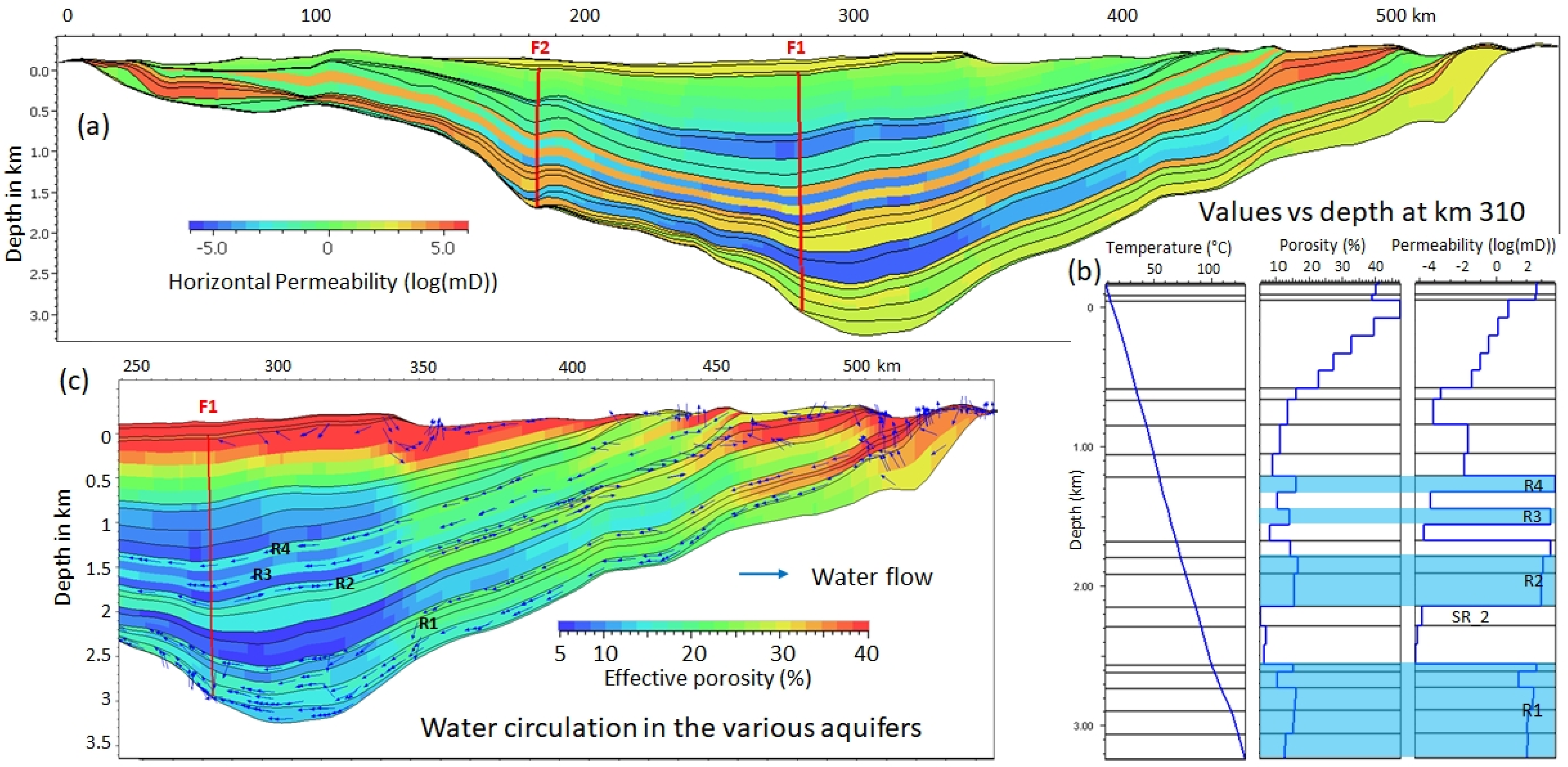
2.2. Methodology Description

This investigation utilizes Petromod© modeling software (2024.2 version) to study the relative role of these transport modes. Petromod© is a basin modeling software which combines seismic, well, and geological information to model the evolution of a sedimentary basin and fluids within. Petromod© models pressure and temperature conditions with n-component/3-phase relationships during the entire migration process [38]. This software works in 1, 2, and 3D but we have here used the 2D version, which is a 3D approach with just a one-kilometer-thick slice. This software, initially designed to model HC generation and migration, has been adapted to compute water transport (advection and diffusion) and gas free phase transport (invasion, percolation, and Darcy flow), parametrized for H2 and other gases. It was this prototype, not yet on the market, that was used.
The geometry shown in Figure 1a represents a 500 km long section of a sedimentary basin with a maximum depth at the depocenter of 3250 m. The series are intercalations of sandstone and shale and a few carbonate layers in the shallow section. The profiles of porosity and permeability at the center of the model (at km 310) can be found in Figure 1b. There is no overpressure in this basin. There is some relief on the right, at around 500 km, which generates a hydraulic load. As three of the aquifers outcrop there, water circulation within these aquifers is strong from right to left, with water flowing downdip in the right and updip in the left of the basin (Figure 1c). One aquifer (R2) is not connected to the surface and therefore not charged by meteoric water; due to its large porosity layer, it channels the compaction water toward the surface, generating an updip water flow.
The geometry is inspired by that of the Paris Basin (the “coupe du centenaire” [44]), but, as already indicated, this article focuses on competition between processes and not on exploration in a given basin. However, one may note that old wells have already been found to have significant concentrations of H2 in the Paris Basin [45]. This H2 is unlikely to be produced within the sedimentary sequence of the basin itself, but rather in its crystalline basement. This modeling work studies how a flow of H2 arriving from the basement is transported within the basin, and where potential accumulations could occur. Since this basin is large and not very deep, all the figures use a significant vertical exaggeration (usually 30), and we would like to draw the reader’s attention to this aspect of the visual rendering.

2.3. Hypotheses

Several constraints and simplifications have been applied to the model in order to focus the discussion on the H2 transport mode. The main ones are as follows:
1‑
Fresh water only. The impact of the initial formation water on the salinity of the water circulating during the last Myr is not taken into account.
2‑
Gas phase is solely H2. The numerical approaches are still limited regarding H2 in the subsurface, and the solubility of a blend, such as CH4 and H2 for instance, is rather unknown, although data show that H2 is not expected to be alone in the gas phase.
3‑
Static geometry. The evolution of the section versus time is not considered. Previous back-stripping allowed for realistic porosity and permeability profiles in the basin. The H2 transport is modeled over 1.5 Myr to 10 Myr. The influx of H2 generated in a deepest zone is constant during a given period ranging from 10 Kyr to 1.5 Myr.
4‑
No biotic H2 generation nor consumption.
5‑
No consumption of H2 by chemical reactions with surrounding rocks.
A sedimentary basin with only fresh water is rather unrealistic, but given that active aquifers are present in the modeled basin [46] and that they lead to a mixing of meteoric and connate waters, this assumption can be considered acceptable. This mainly affects the solubility of H2 and therefore overestimates the role of advection. At 1 km and 50 °C, the solubility of H2 in fresh water is 0.07 mol/kg H2O, while it is 0.06 mol/kg H2O in sea water (0.6 mol NaCl/kg H2O) [38].
Kinetics of H2 generation by redox reactions within the optimal temperature window are faster than HC generation [2,47,48,49]. This has been discussed in the frame of the renewability of H2 [50,51]. It could be slower when the H2 is generated by radiolysis [21] or by the late maturation of organic matter [52]. Since the generation mechanism is not the scope of this paper, a constant rate is assumed.
Microorganisms are not considered in the system. It is well known that certain groups of microbes can readily consume H2 [53,54,55], e.g., methanogenic Archaea; however some authors believe that they can also produce it in significant quantities, especially near the surface [56]. This study does not enter this debate and remains focused on the modes of H2 transport at great depths. In general, a decrease in H2 near the surface can be expected if bacterial consumption is considered.
Finally, other potential losses of H2 by reactions with the beds are not taken into account. This is partially due to the current limitation of the software used, but the few publications regarding H2 reactivity in sandstone and limestone, carried out to evaluate the possibility of storing H2 in such a reservoir, conclude that the reactivity of this gas, alone or blended with CH4, is low [57,58].

2.4. Boundary Conditions

The surface temperature is the average temperature for a latitude of 40° N; this means it is roughly 10 °C today and was less during the quaternary glaciations, and the heat flow at the bottom is chosen constant at 60 mW/m2. Lateral borders are adiabatic. As a result, the maximum temperature at the deepest part is 130 °C. The waterhead is only due to the relief, with the highest point being at 330 m on the right side of the model.
The main parameters of the configurations are summarized in Table 1.
The solubility and diffusion coefficients are from [38] and [59], respectively.
The source intensity, duration, and placement are also varied to appreciate the effect on possible migration paths and the different fluid saturations. H2 is generated first in the center of the deepest layer of the basin, and then on the left and right sides. The H2 generating reaction is not simulated. The injection lasts from 0.5 to 1.5 Myr to today and the quantity is 1–1.5 Mtons/cell, which corresponds to a variable concentration between per 10−4 to 10−2 Mtons/km3/yr (based on matrix volume and due to variable cell shapes and volumes). These values are lower than those expected from laboratory experiments [2] and lower than those measured in field campaigns at the ground surface, which range from 10−4 to 1 Mt/km2/yr [61]. In the specific case of the Campinas structure which has been monitored for 2 years in Brazil, the H2 flow is about 700 kg/day and sincethe SCD is 0.22 km2 large, this means 1160 t/km2/yr [62]. The underestimation of the H2 generation rate is justified for two reasons: (i) the basement may have already released an important part of its H2 yield prior to 1.5 Myr; and (ii) even the release over the last 1.5 Myr quickly saturates the deepest layers, as shown in this study.

2.5. Tested Contexts

The parameters, summarized Table 2, whose influence we tested are as follows:
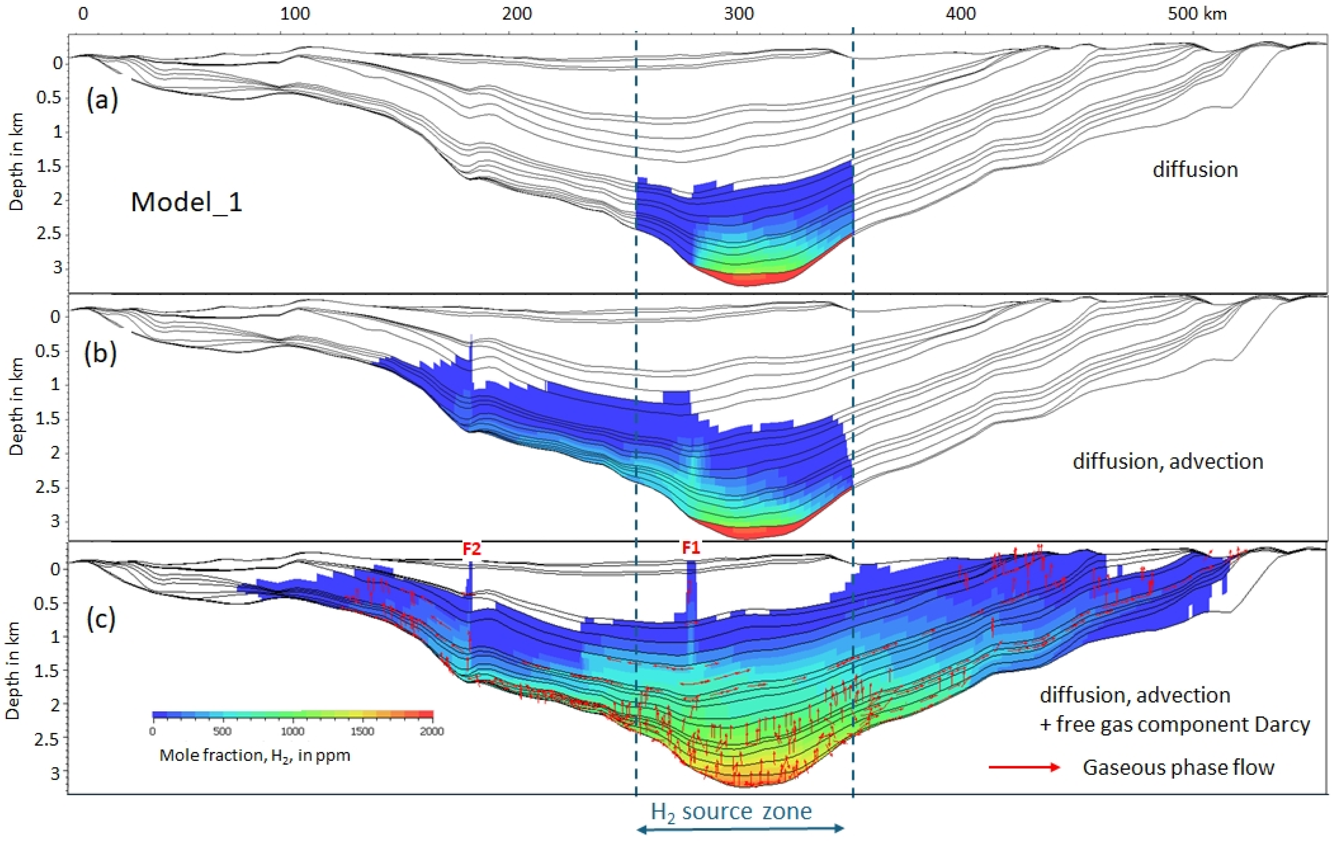
  • Various transport modes: the H2 gaseous phase Darcy flow model was compared to the case with only diffusion and the case with diffusion and advection.
  • H2 kitchen positions: As mentioned, the generation of H2 is not modeled, but the influence of the H2 concentration, duration, and position resulting from this generation is tested through an “injection” of H2 within the model. The source is always in the lowest layer in contact with the basement and placed in three different positions to challenge the aquifer’s importance versus invasion/percolation and to compare the free gas and dissolved H2 paths.
  • The overall quantity of H2 that reaches the bottom of the basin.
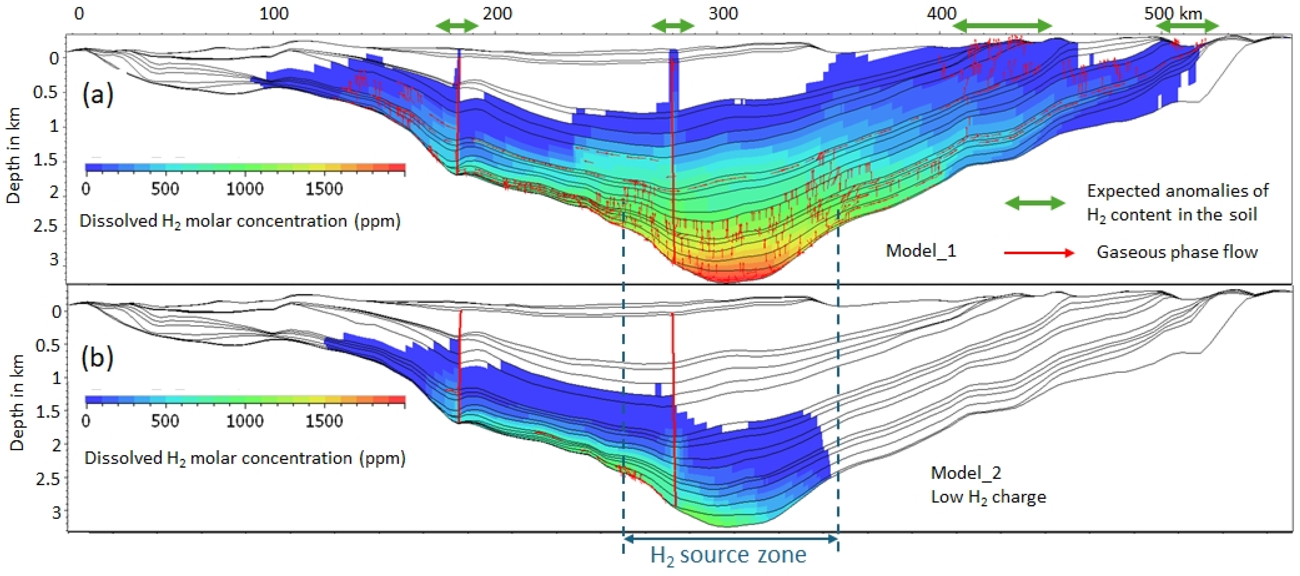
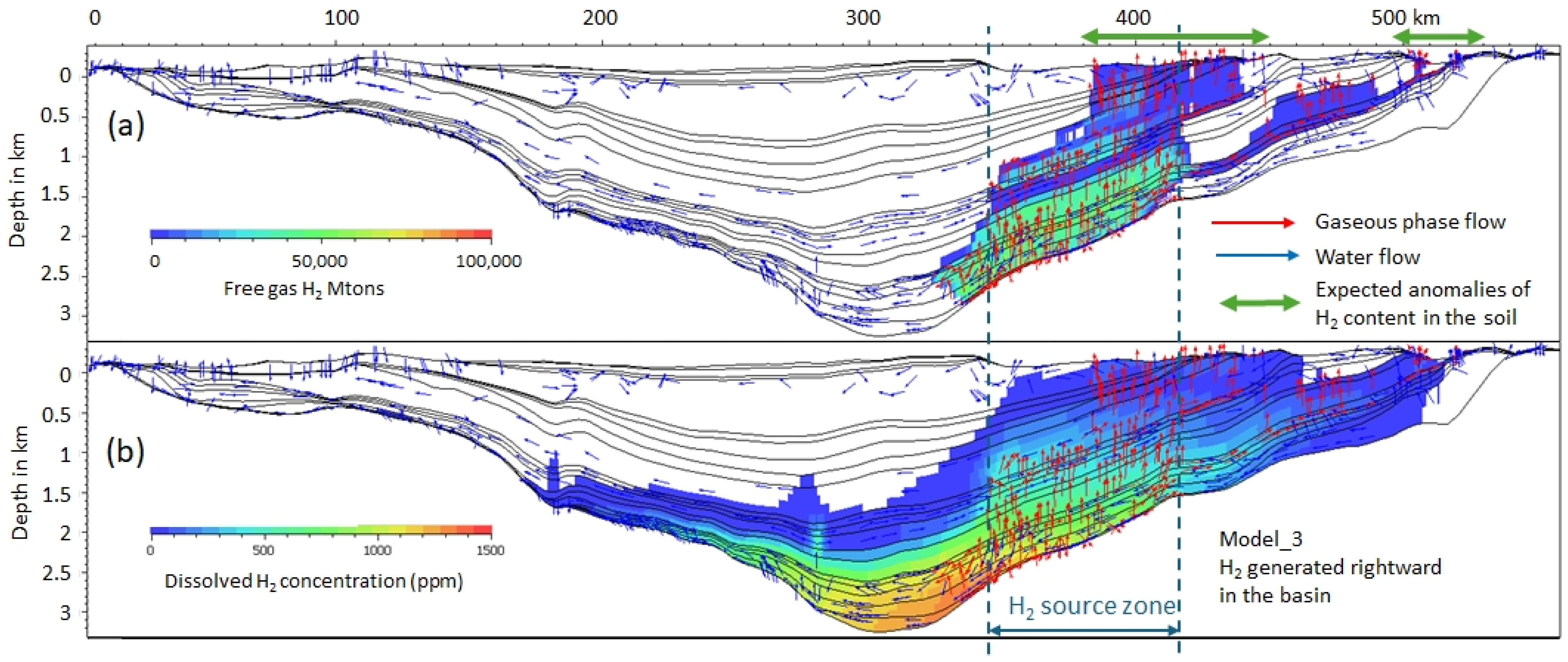
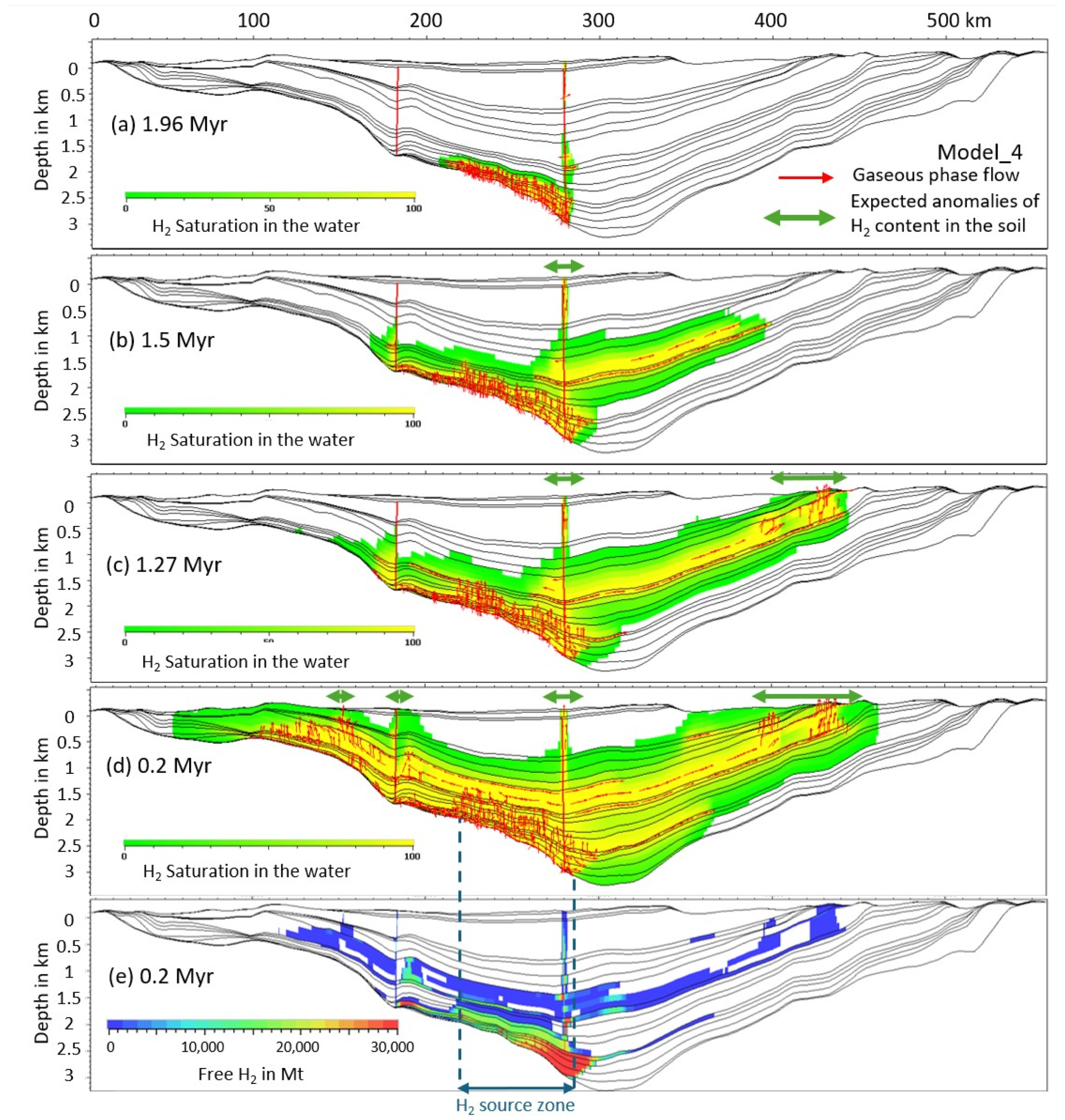
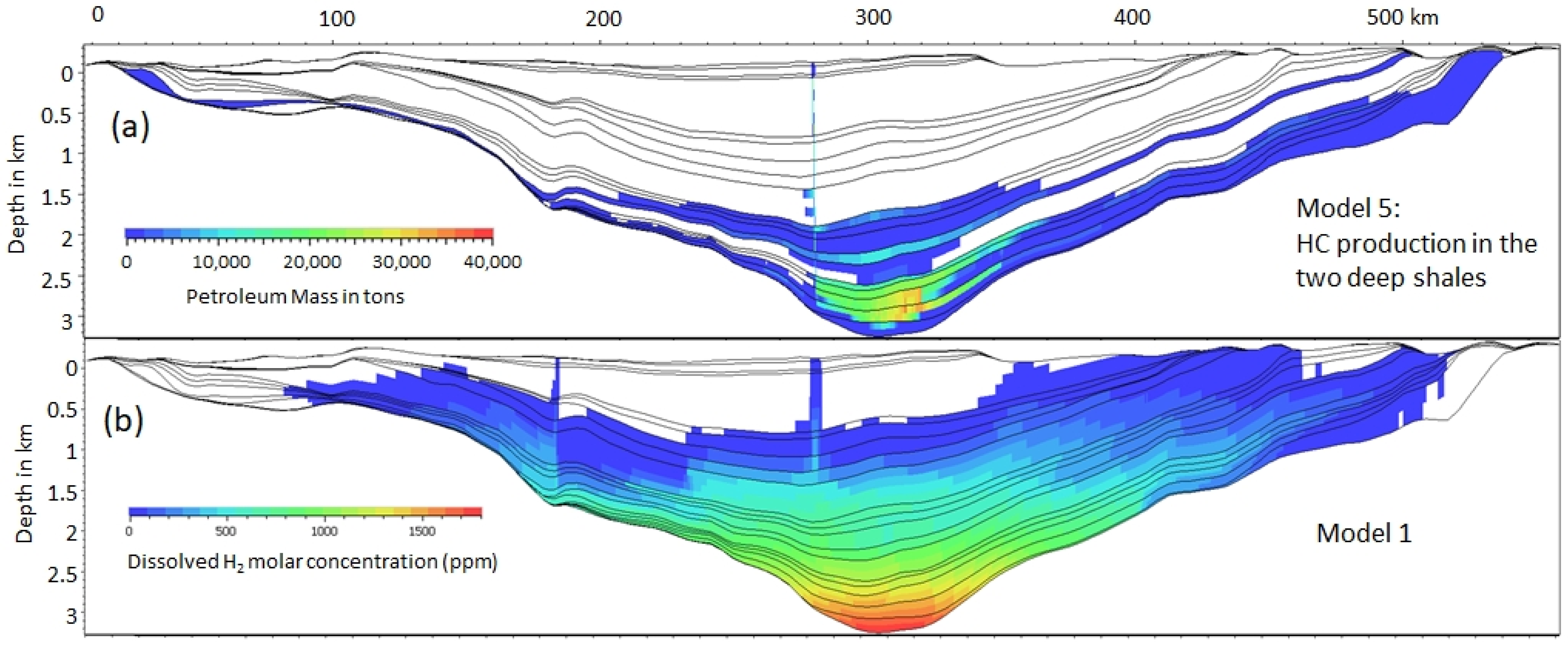
3. Results

3.1. Transport Mode

Figure 2 shows the H2 dissolved in the water at present day, i.e., after a continuous flow of H2 at the deepest part of the basin over 1.5 Myr. When the transport mode is only by diffusion, the displacement is slow, and even after 1.5 million years, the distance traveled by the gas is only around 1.2 km in all directions. As mentioned before, due to the vertical exaggeration of the figure, the lateral diffusion is only visible through the blue lines bordering the H2 plume above the H2 source (Figure 2a). Due to the low solubility of the H2 in water, a large part of the H2 is stuck in the bottom of the section. If the advection is added (Figure 2b), since the water flow is driven by the relief on the right, the water with dissolved H2 is moving toward the left, the H2 follows the same direction.
The H2 content in the cell is expressed in molar ppm and depends on the H2 solubility in water; therefore, there is no direct estimation of the number of kilometers that H2 could cover in 1 Myr, but by the diffusion contribution is small. One kilometer per million years could be considered as an order of magnitude for H2 diffusion in water. Dissolved in water, the H2 has a similar velocity, about 1 m/yr in this study’s case, which means 1000 km in 1 Myr, 1000 times faster than the diffusion.
The videos corresponding to the results of these models versus time can be found in the Supplementary Material.
The free gas is also taken into account in Figure 2c and its displacement is visualized by the red arrows which indicate the direction of the H2 gaseous phase flow. The amount of free gas in the cell is not represented in the background image, which instead shows the concentration of H2 dissolved in water. The H2, as free gas, follows the Darcy flow equation and therefore migrates in the high-permeability zones; in such case the gas also migrates within the aquifer toward the right and invades the right part of the basin, reaching the surface there. The free-flowing gas is consequently in contact with the water in the formations, so dissolved gas is found throughout the right part of the basin due to the free gas displacement in that direction. The H2 reaches the surface at 140 km of the source after 0.7 Myr, corresponding to the average velocity of 2 m/yr. In this case, it is the fastest mode of transportation.
The velocity of the H2’s transport by advection in the aquifer depends on the aquifer velocity, while free gas is faster and reaches the surface thanks to its buoyancy and small molecular size. The surface is not reached in the case of purely diffusive transport mode. In the three transport mode cases (Figure 2c), the average velocity of the advection in the aquifer, except near the surface, is in the range of 10 cm/a, while it is a little bit faster, at 13 cm/a, as free gas. The R1 aquifer has a high permeability of 0.1 Darcy in the lowest central part, resulting in a faster gaseous H2 flow. In addition, the H2 transport is faster in the fault zones, as can be observed in Figure 2c, where water advection increases. When the water charged in H2 reaches the faults that have higher vertical permeability, one notes an efficient and faster upward advection within the faults.
H2 transport therefore involves a continuous transition from the dissolved to the gaseous phase, sometimes several times during H2 ascent to the surface, based on a local dynamic equilibrium. The simplistic image of a gas dissolved at depth and free near the surface is seriously challenged by modeling.
In all the following models the three transport modes are considered.

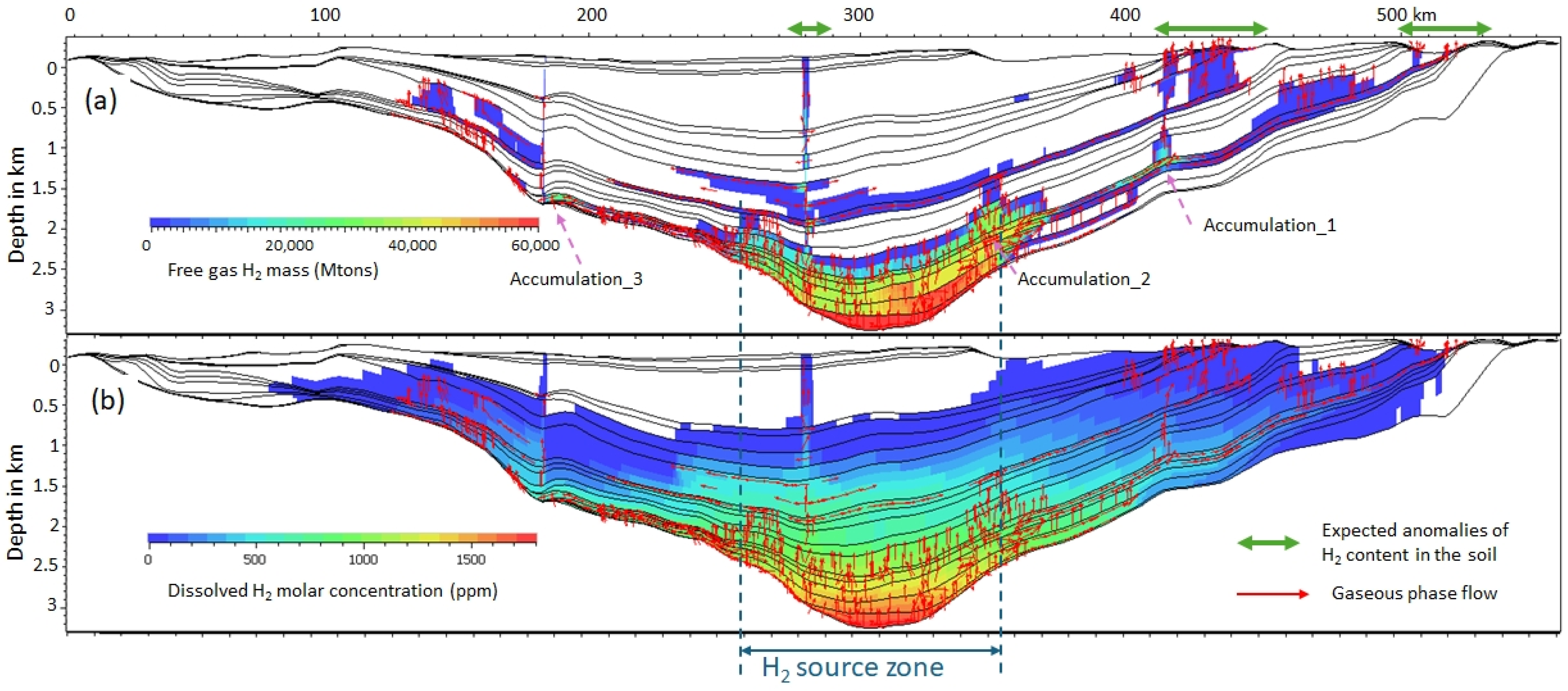
3.2. Dissolved and Free Gas

The color code of the previously displayed figures only included dissolved gas. Figure 3 compares the free gas quantity versus the dissolved. One may observe that free gas is mainly present in the high-porosity carrier beds, R1 and R2, and in the faults. On the left side of the basin, where the advection is dominant, free gas is limited near the H2 source zone. Conversely, on the right side, all the structural traps linked to the slight folds in the reservoirs induce free gas accumulations, even at great depth.
The H2 partition to the gaseous phase appears when the concentration of H2 exceeds the maximum solubility in water at a given depth, temperature, and partial pressure of H2 in the gas phase that is in contact with this liquid phase, according to Henry’s law. In the model the quantities of H2 that will flow in the system are between 1 and 1.5 Mton per cell over 1.5 Myr, which means between 300 and 471 Mt in total during the modeling (Table 2). In comparison with the flow measured in the field, it corresponds to values between 1 and 1400 t/km2/yr, which again are very conservative values [61]. Nonetheless, one may observe in the presented models that even with an active aquifer bordering the H2 source, there is not enough water to dissolve all the H2 (Figure 3b).
The infillings of the three accumulations correspond to a charge at more than 95% in the gaseous phase (accumulation 1: depth of 1350 m in subsoil, free gas, 1.6 kg H2/m3, 0.04 kg H2/m3 dissolved). The charge is slower in the left part of the basin (Accumulation 3, km 188), where the transport by advection is more important (Figure 4). Rapidly the amount of dissolved gas is constant and corresponds to the solubility at that depth.

3.3. Near-Surface Gas and Exsolution

As discussed above, in addition to the dissolved gas, H2 free gas may be present in the cells and migrate as a gaseous phase driven by the pressure gradient and the medium permeability, as described by the Darcy law. The gas phase is present where water becomes oversaturated with dissolved H2. As a result, gaseous H2 may appear, due to exsolution, when the depth of a layer decreases and the pressure drops. Figure 5 shows the actual H2 concentrations for the same modeling scenarios as above but with different H2 bottom flow rates. The red arrows, which describe the displacement of the H2 gaseous phase, clearly show this near-surface exsolution in Figure 5a. In addition to the deep migration in all the carrier beds, the free gas invades the other layers when the solubility decreases. One may expect gas in soil above the shallow aquifers and even in a large part of the basin if the influx of H2 is relatively high. The F1 fault, permeable in this run, serves as a preferential conduit and allows the free gas to reach the surface. High H2 soil gas content may be expected near the outcropping fault zone or above blind faults but also above the aquifers when they are rising toward the surface (Figure 5a).

3.4. Gas Flow Versus Water Flow

The water flow in the aquifers is efficiently promoted if the permeability of their enveloping layers is much lower, i.e., in R3 and R4. In R1 which is the thickest, the flow is the highest towards the top of the bed. The driving force of the flow is the waterhead. Therefore, the water flows downdip, as has been observed in many sedimentary basins, especially in the forelands of mountain belts.
However, the R3 aquifer is not connected to the surface at the right side of the section, due to a pinching out. Hence, it is not charged by meteoric water and its connate water tends to only flow upward.
The gaseous phase of H2 may circulate in the same carrier beds quasi-independently as it is only driven by the gravity and the pressure gradient; hence, it will generally move upward. This could already be observed in Figure 2; yet another scenario has been modeled (Figure 6) with the H2 source zone shifted to the right flank of the basin to observe the phenomenon more closely. Despite the fact that the dissolved gas follows the aquifer and so goes down to the left, the gaseous phase appearance and migration focuses towards the right flank of the basin. Specifically, in R1, one may observe the dissolved gas going in one direction and the free gas in the opposite direction. Another interesting detail to observe in this model is that the area with the maximum dissolved gas concentration (in orange) is not above the active H2 source. This effect is magnified by the increase in H2 solubility with depth.

3.5. H2 Pathway

In tight rock context, the fracture network controls the fluid flow and the H2 flow is focused (by advection and as a free gas) within the faults and their damage zones. However, if a regular carrier bed exists, the quantity of H2 that will use this migration conduit could be much larger than the volume that can pass through the permeable damaged zones surrounding the faults. Although this result is expected and corresponds to what is observed for HC and water circulating in the subsoil, it is important to highlight it. Seeps are often associated with faults (water sources, oil seeps) because these features focus the flow. Yet, in the subsurface, it is the porous and permeable rocks that are the dominating carrier beds. The focusing of flows in narrow zones such as fault zones results in higher concentrations of H2, e.g., in Brazil [32], Australia [33], or Albania [31], signaling an active H2 system at depth and implying that the source might be directly down the fault plane. However, the fault could also be only a secondary migration path, e.g., cutting through a carrier bed, and not directly linked to an accumulation or the active source.
As mentioned above, a point highlighted by this modeling and which is perhaps less intuitive is that dissolved gas can move in the opposite direction to free gas. In the presented case, three of the aquifers are moving from right to left due to the waterhead effect of the reliefs. As a result, the dissolved gas within is moving toward the left. The free gas follows the slope updip and for a large part migrates to the right in the studied geometry. The diffusion is not very efficient, and rather slow if there is no high-pressure build up and if it is the only transport mode and the H2 remains in the vicinity of the H2 source zone.
The conclusions of this work should not be taken as being representative of a specific basin, even if the geometry is derived from that of the Paris Basin framework. This is a parametric approach using the geologic and structural framework of a well-known basin to study the effects of certain causes. Yet, qualitative or semiquantitative conclusions could be discussed based on this numerical approach. These two points, the fact that H2 can go down in a basin with aquifers when it is dissolved and can oppositely rise “against the current” as free gas in an aquifer, are to be taken into account when thinking about the drainage area of a given trap.
In cases where the aquifers do not all flow in the same direction, and the Darcean gas flow is in a different direction, the H2 can be dispersed throughout the basin. Such a context reduces the Probability of Success (POS) of finding large accumulations. A 3D approach taking into account the drainage area and the specific geometry of a structure will be necessary to quantify load and recharge. Knowledge of aquifer velocities will also be an important parameter.

3.6. H2 in the Near-Surface Soils and Beds

If the H2 charge is large, all the aquifers may be rich in dissolved gas and may even contain a free gas phase (Figure 2c, Figure 3, and Figure 4). Some H2 leakage may be, in that case, expected in large surface areas. As for the H2 leakage via faults, the H2 content in the soil does not give definitive indications regarding the accumulation, but clearly indicates that deep aquifers are saturated in H2 and therefore that a H2 system is active in the zone. Accumulations are to be sought in structural traps not directly under the surface emanations but on the migration path where the reservoir/carrier beds are at greater depths.
Above an accumulation, sealed off by good-quality cap rock, it is not certain that gaseous leakage will be present, but it cannot be precluded [50], similarly to traps of gaseous HCs [63]. In the modeling performed here, there is leakage above certain accumulations (when the free gas load exceeds 42,000 Mt per cell, Figure 3) but it can be noted that the rising H2 flow dissolves in the aquifers above the accumulation and is therefore diverted before reaching the surface.
Above blind faults, H2 leakages are much more likely. Fairy circles/subcircular depressions (SCDs) with high H2 content have been observed in Russia [64] and these authors suggested the presence of faults to explain the alignment of these structures. Similarly, in the French Pyrenean foreland where H2 has been noted in the soil, the influence of faults, and the difference between the hanging wall and the footwall of blind faults in terms of H2 content, have also been highlighted [65].
If we compare the three models with different source positions, we can observe that the area, or the length in this 2D model, where H2 is expected in the ground is 60 km long for Model 1, 95 km for Model_3, and 20 km for Model_4. When the H2 generation is low, as in Model_2, there is no H2 reaching the ground surface. These zones of near-surface H2 anomalies are mostly located on the right-hand side of the basin, where free gas transport is predominant, which results in a greater H2 quantity, even when the source is on the other side.
Overall, the soil transport model presented here confirms that in a sedimentary basin, the more H2 there is at depth, the more is found in the near-surface soil. A first step of prospecting based on the use of soil gas, or on the trace of soil gas anomalies like the SCD or vegetation anomalies, therefore remains relevant. This model suggests that if the H2 presence is restricted to fault zones or aquifer outcrops, the H2 system is probably less rich.

3.7. Expected Distance Between the H2 Kitchen, the H2 Accumulation, and the H2 Seeps

Many visual representations of H2 systems show mainly vertical H2 displacement in the subsurface [3] or just advection in fault zones [66]. The modeling shown here confirms that the H2 transport is much more complex. It follows the rules of movement of all fluids in the subsurface, i.e., it follows the “easiest” path, which is almost never vertical in a stratified and faulted environment. The fluid path may cover, horizontally, hundreds of kilometers, especially in the foreland where the pressure gradient due to the relief is large. In Colombia, a modeling of the H2 transport in the Llanos Basin, the foreland of the current Eastern Cordillera, has been performed and it was also concluded that the transport of H2 could justify exploration for H2 reserves in the eastern external part of the foreland [67]. In that basin, structural traps exist on faulted blocks, affecting the carrier beds (the various sandstones in that case), but also stratigraphic traps on the pinch out of the series eastward. The oil migration took place over a large distance from a 200 km distant HC kitchen near the Cordillera [68]. The H2 may follow the same pathway and even local generation may exist eastward, closer to the traps that contain known HC accumulations [67].

3.8. Depth of Exsolution

When looking for an accumulation of H2 that could enable economic production, finding a free gas phase and not just H2 dissolved in water is a game-changing factor. In Mali, in Bourakebougou, data have shown a dry gas in the discovery of a shallow well (110 m depth) but also the bubbling of gas during drilling into the deepest levels down to 2 km [10,69]. The exsolution takes place when the amount of H2 exceeds the solubility. Figure 7 shows where this saturation took place in the case of a H2-generating zone situated on the left side of the basin (Model_4, Table 2). About 1.8 Myr are required for the H2 to reach the surface; the 0.2 Myr stage was chosen for this display because this is when H2 begins to reach the surface.
Conversely, if at the basin scale a free gas phase arrives in contact with undersaturated water, the H2 will partition into the dissolved phase, potentially changing its migration fate. Additional information about the H2 source and therefore possible migration mechanisms and routes can be studied using hydrogen’s stable isotopes and noble gases. However, the H2 isotope analyses alone can be ambiguous for directly inferring the source of H2, as they rather indicate a temperature of equilibrium [7]. Noble gas and nitrogen isotope analyses indicate an open system in the H2-rich basin with a strong exchange with the aquifers [70], also confirmed by the modeling presented here. The latter publication proposes a temperature around 70 °C for the exsolution of the H2 corresponding to circa 2 km, which is also similar to this study’s findings, pending many controls other than pressure and temperature which can impact the solubility. One of the important parameters that influences the H2 solubility in water is the presence of other gases, as it has been studied for N2, CO2, CH4, and He blends. Therefore a precise knowledge of the gas mixture is key to quantify exsolution conditions [41].

4. Conclusions/Perspectives

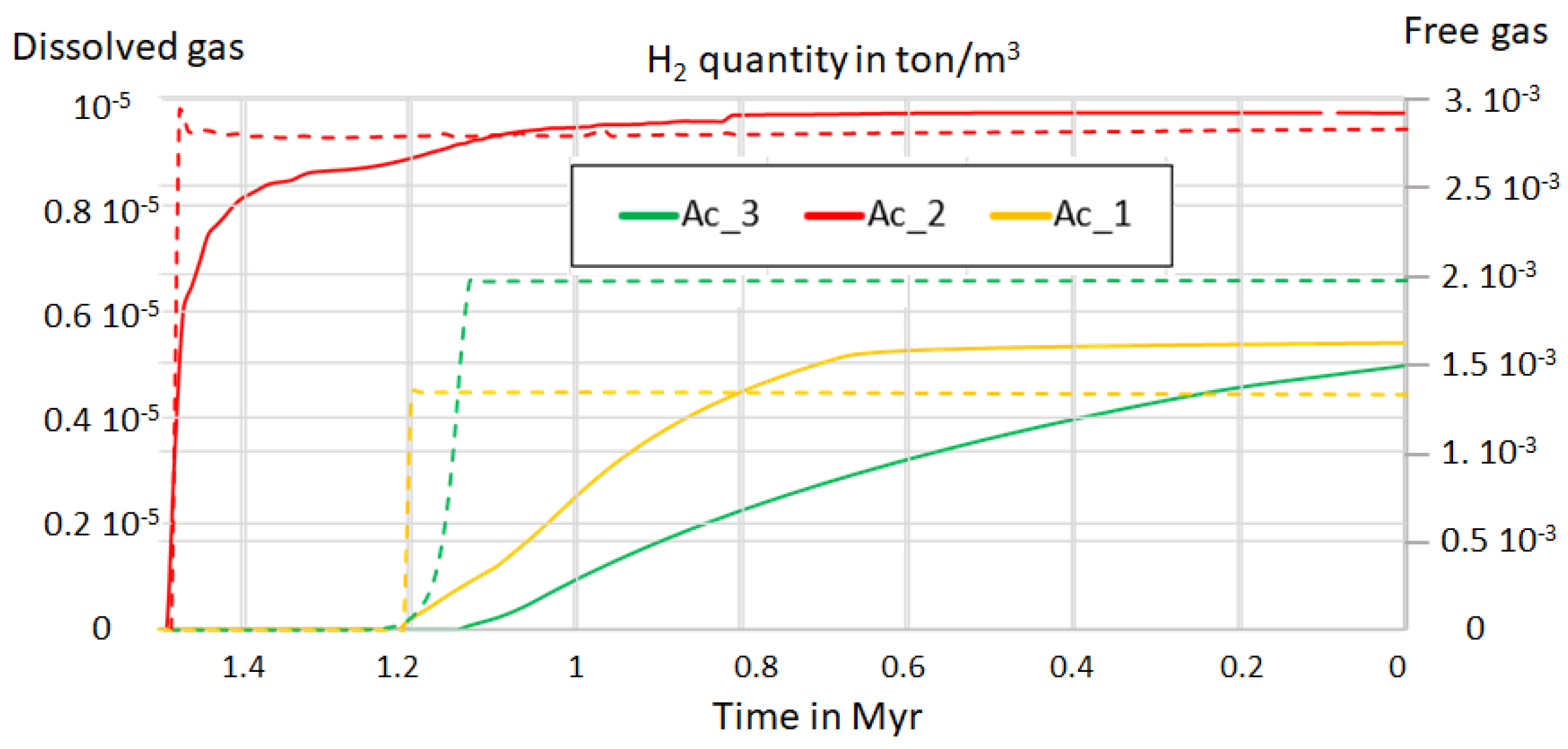
4.1. Fossil vs. Dynamic Accumulations

Economic accumulation of H2 will very likely be linked to free gas accumulation [71]. For the exploration companies, being able to prove reserves in order to design the production facility is mandatory. A dynamic system with a constant recharge as observed in Mali [69] will be a bonus but it is unlikely that the initial data set available before the investment decision will allow such an optimistic hypothesis. However, the presented parametric quantification of the H2 transport in a basin and the resulting H2 flows suggest that a dynamic aquifer may indeed recharge a trap with free gas. If the water flow in the aquifer is slow, at a human lifetime scale, the H2 reservoir rate of recharge may be negligible, yet quantifiable by numerical models. A good knowledge of the drainage area of the relief morphology and the geometry of subsurface structures can constrain the water fluxes and their flow vectors in a basin. Knowing that huge resources of H2 have been generated and continue to be generated in the lithosphere [8], the question of renewable versus fossil energy sources for natural H2 is, in our point of view, not the right one. Many of the reactions that generate H2 are not reversible, but oxidoreduction and radiolysis affect a huge volume of rocks (almost all the crust). The recycling between Fe2+ and Fe3+ exists, but happens in the subduction zone and therefore over long geological cycles [72]. The key question to answer today is, however, can we have long-term H2 production from the same well, or a set of wells within an entire field? The answer is positive in Mali, but the production rate is limited [69]; elsewhere it remains unknown.
Joint modeling with aquifers and a free gas phase shows a dynamic system, with accumulations filling up within the first 2 million years after the start of H2 generation at depth. Then, in the case studied, there is a balance between leakage and filling. The H2-saturated aquifer continues to deliver a flow of H2 that outgasses the structure and compensates for the gas leaking through the cover clays. This recharge role played by the aquifer, for example with regard to accumulation 1 in Figure 3a, is partly due to the monoclinal geometry of the basin. A closed anticline-type structural trap without active water recharge certainly does not behave in the same way, but this is the model proposed for Mali, with small reservoirs scattered along a monocline [10,69]. A dynamic system with constant recharge could therefore be fairly common for H2, but the speed of this recharge rather than the speed of generation will depend on the speed of the aquifers and the displacement of the gas. Fast for a geological phenomenon does not mean it will occur in a few years.
Another study has recently been proposed, based on a comparison between H2 generation rates and those required for economic production [51]. The authors consider that H2 would be renewable if these two values were equal. As their model is only 1D, the drainage area is not modeled, and is arbitrarily set at 10 km by the authors. The 2D modeling (pseudo 3D) performed here shows the possibility that much larger drainage area H2 flows from hundreds of kilometers away can converge on the same structure resulting in stronger recharge.
Now, however, the numerical models, as shown here, could shed light on such potential, especially with rapidly growing calibration data sets. Specifically, discovery well inputs into the coupling between the reservoir scale and the basin scale will be necessary.

4.2. Transport Model Scheme

There are similarities between the transport of H2 in the subsurface and the transport of any fluid, but due to its solubility, and to a lesser extent, due to its diffusivity, the classical models we have in mind could prove to be wrong. On the one hand, these models are often too simplistic (limited mechanisms of gas transport and inadequate parametrization), and they are often based solely on hydraulic or petroleum system processes which are modeled for more than a half century. Figure 8 shows a comparison of the HC charge and the H2 charge in the studied basin. The computation has been performed over the 250 Myr of the basin’s history for the HC, since the kinetics of generation is slower.
An evident similarity with the HC system is that the H2, even as a free gas, does not predominantly go up vertically. Therefore, a long-distance migration can be considered a common feature in sedimentary basins. As a result, a map view of the prospectivity could be misleading, and the drainage area of each individual play has to be computed. HC or H2 gas accumulations can form in similar structural traps below a seal or lateral barriers. If the H2 reaches the traps as a free gas, the reservoir will typically fill up over time. However, if the H2 is dissolved in the water, a slowing down of the water flow, due, for instance, to the trap geometry, will also affect the H2 flow. In the absence of a gas phase, the quantity of H2 will be limited by the solubility.
If not stopped by a trap, an oil phase rather immiscible with water will follow the carrier bed toward the surface. The H2 dissolved will follow the water flow and could be transported toward the opposite direction. As a result of these different modes of transport and its solubility, H2 invades a large part of the basin’s sedimentary series. Accumulations are punctual, but the presence of H2 in small quantities everywhere can give the impression that its presence is dispersed and ubiquitous. Accumulations are not expected to be widespread; good imaging, e.g., seismic surveys, of the subsurface will be necessary for successful exploration.

4.3. Accounting for H2 Consumption in the Subsurface

It should be remembered that the calculations made here represent H2 transport in a sedimentary basin with porous and fairly active aquifers, even if the surrounding relief and therefore the hydraulic load are not very high. The fact that bacterial consumption is not considered leads to a higher presence of gas in near-surface soils, but has no influence on the placement of these emissions. The subsurface biosphere microbial activity is expected to consume H2 at a certain speed [53], and despite limited quantifications, could be introduced in a more advanced version of the software. This implementation would certainly reduce the amount of H2 near the surface. However, it should be kept in mind that bacterial consumption is only active relatively close to the surface, and the data published in Brazil only concern the first meter of soil. In contrast, as the temperature passes 120 °C, the microbial communities disappear [55]. Recent modeling work on H2 consumption by microorganisms in a reservoir concludes that the impact is negligible to low, at less than 3% after a tens of years [73]. This last work is carried out on depleted HC fields, taking into account methanogenesis, homoacetogenesis, and sulfate reduction; the authors conclude that these reservoirs are perfectly suitable for underground H2 storage. The chemical reactivity of H2 dismissed in our study will nevertheless also limit the residence time of H2 in the basins.

4.4. Exploration Strategy

In conclusion, this parametric approach showed that basin modeling will also be useful for H2 exploration. Based on a well-defined geometry and knowing the H2_GR, hydrogeology, with supporting calibration data (H2 phase and concentration measurements in the soil and in the subsurface, e.g., exploration well, water wells, etc.) allows the prediction of the accumulation more accurately. In addition, the simplified case presented here provides a better understanding of the relationship between aquifers, faults, and surface emissions. Results confirm the value of gas sampling in the early stages of H2 exploration but also show that surface emanations are rarely directly above accumulations. Even in the case of dismigration from a H2 accumulation, shallower aquifers can divert the gas flow.
Based on this work, one can anticipate that a H2_GR below a sedimentary basin will result in larger accumulations than H2 in just a tight, old, fractured cratonic basin and that free gas accumulation will not be limited to the first hundred meters.
In terms of data acquisition when doing H2 prospection, the numerical approach shown here suggests the following:
Existence of H2 in the soil is a relevant proxy to prove the existence of an active H2 system.
The size of the region with emanations is related to the importance of the deep H2 charge.
The SCD density map should be compared with the aquifer map, but the SCDs’ positions are not particularly relevant to locate an accumulation.
The measurement of dissolved H2 in the aquifer should be performed more systematically to confirm the presence of a H2 deep flow. Measurements at different depths to verify whether or not the water is systematically saturated with H2 would be useful.
If degassing occurs above an aquifer, geophysical acquisitions should be targeted to find a play in the part of the basin where the aquifer is deeper. The flow of the water must be between the expected H2-generating zone and the SCDs.
The water flow must be directed from the generation zone to the target, but the POS is better if the free gas flow follows the same path.
An active H2-charged aquifer may continuously recharge the reservoirs.
Now that modeling is possible, it seems important to perform it specifically for each basin to reduce the risk of H2 exploration, even if a lot of data are still missing for it to be completely predictive.

Supplementary Materials

The following supporting information can be downloaded at: https://www.mdpi.com/article/10.3390/geosciences15080298/s1, A total of 14 videos are shared corresponding to the H2 displacement and accumulation in the basin depending of the various models (1 to 4) as well as the HC displacement (Model 5). For each model, dissolved gas in ppm, free gas in Mtons and saturation in % are displayed. Since the software interface is not yet finalized, some of the inscriptions on the films, particularly the captions, are incorrect. Please refer to the figures in the article for details of the values.

Author Contributions

Conceptualization, L.N. and I.M.; methodology, all; validation, all; investigation, L.N.; data curation, L.N. and J.C.H.; writing—original draft preparation, I.M.; writing—review and editing, L.N., I.M., J.C.H., and D.S.; visualization, L.N. and I.M. All authors have read and agreed to the published version of the manuscript.

Funding

This research received no external funding.

Data Availability Statement

No new data were created but the results of the various modeling versus time plots are available in the Supplementary Material.

Acknowledgments

This work benefited from discussions with Vincent Roche. With thanks to Benjamin Bruneau for the horizon data set and discussion around the Paris Basin.

Conflicts of Interest

Author Juan Carlos Hidalgo and Dariusz Strąpoć are employed by the company SLB. The remaining authors declare that the research was conducted in the absence of any commercial or financial relationships that could be construed as a potential conflict of interest.

Abbreviations

The following abbreviations are used in this manuscript:
SCDSubcircular Depression
H2_GRGenerating Rock in H2 System
HCHydrocarbon
SRSource Rock in HC System
TOCTotal Organic Carbon
POSProbability of Success

References

  1. Truche, L.; McCollom, T.M.; Martinez, I. Hydrogen and Abiotic Hydrocarbons: Molecules That Change the World. Elements 2020, 16, 13–18. [Google Scholar] [CrossRef]
  2. Lévy, D.; Roche, V.; Pasquet, G.; Combaudon, V.; Geymond, U.; Loiseau, K.; Moretti, I. Natural H2 Exploration: Tools and Workflows to Characterize a Play. Sci. Technol. Energy Transit. 2023, 78, 27. [Google Scholar] [CrossRef]
  3. Hand, E. Hidden Hydrogen. Science 2023, 379, 630–636. [Google Scholar] [CrossRef] [PubMed]
  4. Gaucher, E.C.; Moretti, I.; Pélissier, N.; Burridge, G.; Gonthier, N. The Place of Natural Hydrogen in the Energy Transition: A Position Paper. Eur. Geol. 2023, 55, 5–9. [Google Scholar] [CrossRef]
  5. Brandt, A.R. Greenhouse Gas Intensity of Natural Hydrogen Produced from Subsurface Geologic Accumulations. Joule 2023, 7, 1818–1831. [Google Scholar] [CrossRef]
  6. Mathur, Y.; Moise, H.; Aydin, Y.; Mukerji, T. Techno-Economic Analysis of Natural and Stimulated Geological Hydrogen. Nat. Rev. Earth Environ. 2025, 6, 342–356. [Google Scholar] [CrossRef]
  7. Boreham, C.J.; Edwards, D.S.; Czado, K.; Rollet, N.; Wang, L.; van der Wielen, S.; Champion, D.; Blewett, R.; Feitz, A.; Henson, P.A. Hydrogen in Australian Natural Gas: Occurrences, Sources and Resources. APPEA J. 2021, 61, 163. [Google Scholar] [CrossRef]
  8. Ellis, G.S.; Gelman, S.E. Model Predictions of Global Geologic Hydrogen Resources. Sci. Adv. 2024, 10, eado0955. [Google Scholar] [CrossRef]
  9. Prinzhofer, A.; Tahara Cissé, C.S.; Diallo, A.B. Discovery of a Large Accumulation of Natural Hydrogen in Bourakebougou (Mali). Int. J. Hydrogen Energy 2018, 43, 19315–19326. [Google Scholar] [CrossRef]
  10. Maiga, O.; Deville, E.; Laval, J.; Prinzhofer, A.; Diallo, A.B. Trapping Processes of Large Volumes of Natural Hydrogen in the Subsurface: The Emblematic Case of the Bourakebougou H2 Field in Mali. Int. J. Hydrogen Energy 2024, 50, 640–647. [Google Scholar] [CrossRef]
  11. Jackson, O.; Lawrence, S.R.; Hutchinson, I.P.; Stocks, A.E.; Barnicoat, A.C.; Powney, M. Natural Hydrogen: Sources, Systems and Exploration Plays. Geoenergy 2024, 2, geoenergy2024-002. [Google Scholar] [CrossRef]
  12. Klein, F.; Tarnas, J.D.; Bach, W. Abiotic Sources of Molecular Hydrogen on Earth. Elements 2020, 16, 19–24. [Google Scholar] [CrossRef]
  13. Zgonnik, V. The Occurrence and Geoscience of Natural Hydrogen: A Comprehensive Review. Earth Sci. Rev. 2020, 203, 103140. [Google Scholar] [CrossRef]
  14. Leila, M.; Loiseau, K.; Moretti, I. Controls on Generation and Accumulation of Blended Gases (CH4/H2/He) in the Neoproterozoic Amadeus Basin, Australia. Mar. Pet. Geol. 2022, 140, 105643. [Google Scholar] [CrossRef]
  15. Coveney, R.M., Jr.; Goebel, E.D.; Zeller, E.; Dreschhoff, G. Serpentinization and the Origin of Hydrogen Gas in Kansas. Bulletin 1987, 71, 39–48. [Google Scholar] [CrossRef]
  16. De Freitas, V.A.; Prinzhofer, A.; Françolin, J.B.; Ferreira, F.J.F.; Moretti, I. Natural Hydrogen System Evaluation in the São Francisco Basin (Brazil). Sci. Technol. Energy Transit. 2024, 79, 95. [Google Scholar] [CrossRef]
  17. Murray, J.; Clément, A.; Fritz, B.; Schmittbuhl, J.; Bordmann, V.; Fleury, J.M. Abiotic Hydrogen Generation from Biotite-Rich Granite: A Case Study of the Soultz-Sous-Forêts Geothermal Site, France. Appl. Geochem. 2020, 119, 104631. [Google Scholar] [CrossRef]
  18. Horsfield, B.; Mahlstedt, N.; Weniger, P.; Misch, D.; Vranjes-Wessely, S.; Han, S.; Wang, C. Molecular Hydrogen from Organic Sources in the Deep Songliao Basin, P.R. China. Int. J. Hydrogen Energy 2022, 47, 16750–16774. [Google Scholar] [CrossRef]
  19. Wang, L.; Jin, Z.; Chen, X.; Su, Y.; Huang, X. The Origin and Occurrence of Natural Hydrogen. Energies 2023, 16, 2400. [Google Scholar] [CrossRef]
  20. Boreham, C.J.; Edwards, D.S.; Feitz, A.J.; Murray, A.P.; Mahlstedt, N.; Horsfield, B. Modelling of Hydrogen Gas Generation from Overmature Organic Matter in the Cooper Basin, Australia. APPEA J. 2023, 63, S351–S356. [Google Scholar] [CrossRef]
  21. Lollar, B.S.; Onstott, T.C.; Lacrampe-Couloume, G.; Ballentine, C.J. The Contribution of the Precambrian Continental Lithosphere to Global H2 Production. Nature 2014, 516, 379–382. [Google Scholar] [CrossRef] [PubMed]
  22. Deville, E.; Prinzhofer, A. The Origin of N2-H2-CH4-Rich Natural Gas Seepages in Ophiolitic Context: A Major and Noble Gases Study of Fluid Seepages in New Caledonia. Chem. Geol. 2016, 440, 139–147. [Google Scholar] [CrossRef]
  23. Vacquand, C.; Deville, E.; Beaumont, V.; Guyot, F.; Sissmann, O.; Pillot, D.; Arcilla, C.; Prinzhofer, A. Reduced Gas Seepages in Ophiolitic Complexes: Evidences for Multiple Origins of the H2-CH4-N2 Gas Mixtures. Geochim. Cosmochim. Acta 2018, 223, 437–461. [Google Scholar] [CrossRef]
  24. Leong, J.A.; Nielsen, M.; McQueen, N.; Karolytė, R.; Hillegonds, D.J.; Ballentine, C.; Darrah, T.; McGillis, W.; Kelemen, P. H2 and CH4 Outgassing Rates in the Samail Ophiolite, Oman: Implications for Low-Temperature, Continental Serpentinization Rates. Geochim. Cosmochim. Acta 2023, 347, 1–15. [Google Scholar] [CrossRef]
  25. Palmowski, D.; Fernandez, N.; Kleine, A.; Lefeuvre, N.; Tari, G. Modelling Natural Hydrogen Systems. Extending the Basin Modeler’s Comfort Zone. In Proceedings of the 85th EAGE Annual Conference & Exhibition (including the Workshop Programme), Oslo, Norway, 10–13 June 2024; European Association of Geoscientists & Engineers: Utrecht, The Netherlands, 2024. [Google Scholar]
  26. Zgonnik, V.; Beaumont, V.; Deville, E.; Larin, N.; Pillot, D.; Farrell, K.M. Evidence for Natural Molecular Hydrogen Seepage Associated with Carolina Bays (Surficial, Ovoid Depressions on the Atlantic Coastal Plain, Province of the USA). Prog. Earth Planet. Sci. 2015, 2, 31. [Google Scholar] [CrossRef]
  27. Moretti, I.; Brouilly, E.; Loiseau, K.; Prinzhofer, A.; Deville, E. Hydrogen Emanations in Intracratonic Areas: New Guide Lines for Early Exploration Basin Screening. Geosciences 2021, 11, 145. [Google Scholar] [CrossRef]
  28. Roche, V.; Geymond, U.; Boka-Mene, M.; Delcourt, N.; Portier, E.; Revillon, S.; Moretti, I. A New Continental Hydrogen Play in Damara Belt (Namibia). Sci. Rep. 2024, 14, 11655. [Google Scholar] [CrossRef]
  29. Ginzburg, N.; Daynac, J.; Hesni, S.; Geymond, U.; Roche, V. Identification of Natural Hydrogen Seeps: Leveraging AI for Automated Classification of Sub-Circular Depressions. Earth Space Sci. 2025, 12, e2025EA004227. [Google Scholar] [CrossRef]
  30. Pasquet, G.; Houssein Hassan, R.; Sissmann, O.; Varet, J.; Moretti, I. An Attempt to Study Natural H2 Resources across an Oceanic Ridge Penetrating a Continent: The Asal–Ghoubbet Rift (Republic of Djibouti). Geosciences 2021, 12, 16. [Google Scholar] [CrossRef]
  31. Truche, L.; Donzé, F.-V.; Goskolli, E.; Muceku, B.; Loisy, C.; Monnin, C.; Dutoit, H.; Cerepi, A. A Deep Reservoir for Hydrogen Drives Intense Degassing in the Bulqizë Ophiolite. Science 2024, 383, 618–621. [Google Scholar] [CrossRef]
  32. Prinzhofer, A.; Rigollet, C.; Lefeuvre, N.; Françolin, J.; Valadão De Miranda, P.E. Maricá (Brazil), the New Natural Hydrogen Play Which Changes the Paradigm of Hydrogen Exploration. Int. J. Hydrogen Energy 2024, 62, 91–98. [Google Scholar] [CrossRef]
  33. Frery, E.; Langhi, L.; Maison, M.; Moretti, I. Natural Hydrogen Seeps Identified in the North Perth Basin, Western Australia. Int. J. Hydrogen Energy 2021, 46, 31158–31173. [Google Scholar] [CrossRef]
  34. Vrolijk, P.J.; Urai, J.L.; Kettermann, M. Clay Smear: Review of Mechanisms and Applications. J. Struct. Geol. 2016, 86, 95–152. [Google Scholar] [CrossRef]
  35. Moretti, I.; Labaume, P.; Sheppard, S.M.F.; Boulègue, J. Compartmentalisation of Fluid Migration Pathways in the Sub-Andean Zone, Bolivia. Tectonophysics 2002, 348, 5–24. [Google Scholar] [CrossRef]
  36. Faulkner, D.R.; Jackson, C.A.L.; Lunn, R.J.; Schlische, R.W.; Shipton, Z.K.; Wibberley, C.A.J.; Withjack, M.O. A Review of Recent Developments Concerning the Structure, Mechanics and Fluid Flow Properties of Fault Zones. J. Struct. Geol. 2010, 32, 1557–1575. [Google Scholar] [CrossRef]
  37. Akinfiev, N.N.; Diamond, L.W. Thermodynamic Description of Aqueous Nonelectrolytes at Infinite Dilution over a Wide Range of State Parameters. Geochim. Cosmochim. Acta 2003, 67, 613–629. [Google Scholar] [CrossRef]
  38. Lopez-Lazaro, C.; Bachaud, P.; Moretti, I.; Ferrando, N. Predicting the Phase Behavior of Hydrogen in NaCl Brines by Molecular Simulation for Geological Applications. BSGF Earth Sci. Bull. 2019, 190, 7. [Google Scholar] [CrossRef]
  39. Strauch, B.; Pilz, P.; Hierold, J.; Zimmer, M. Experimental Simulations of Hydrogen Migration through Potential Storage Rocks. Int. J. Hydrogen Energy 2023, 48, 25808–25820. [Google Scholar] [CrossRef]
  40. Ehhalt, D.H.; Rohrer, F. The Tropospheric Cycle of H2: A Critical Review. Tellus B Chem. Phys. Meteorol. 2009, 61, 500. [Google Scholar] [CrossRef]
  41. Cheng, A.; Sherwood Lollar, B.; Gluyas, J.G.; Ballentine, C.J. Primary N2–He Gas Field Formation in Intracratonic Sedimentary Basins. Nature 2023, 615, 94–99. [Google Scholar] [CrossRef]
  42. Bossennec, C.; Géraud, Y.; Böcker, J.; Klug, B.; Mattioni, L.; Bertrand, L.; Moretti, I. Characterisation of Fluid Flow Conditions and Paths in the Buntsandstein Gp. Sandstones Reservoirs, Upper Rhine Graben. BSGF Earth Sci. Bull. 2021, 192, 35. [Google Scholar] [CrossRef]
  43. Hantschel, T.; Kauerauf, A. Fundamentals of Basin and Petroleum Systems Modeling; Springer: Berlin/Heidelberg, Germany, 2009; ISBN 978-3-540-72317-2. [Google Scholar]
  44. Mas, P.; Calcagno, P.; Caritg-Monnot, S.; Beccaletto, L.; Capar, L.; Hamm, V. A 3D Geomodel of the Deep Aquifers in the Orléans Area of the Southern Paris Basin (France). Sci. Data 2022, 9, 781. [Google Scholar] [CrossRef]
  45. Lefeuvre, N.; Thomas, E.; Truche, L.; Donzé, F.; Cros, T.; Dupuy, J.; Pinzon-Rincon, L.; Rigollet, C. Characterizing Natural Hydrogen Occurrences in the Paris Basin From Historical Drilling Records. Geochem. Geophys. Geosyst 2024, 25, e2024GC011501. [Google Scholar] [CrossRef]
  46. De Hoyos, A.; Viennot, P.; Ledoux, E.; Matray, J.-M.; Rocher, M.; Certes, C. Influence of Thermohaline Effects on Groundwater Modelling–Application to the Paris Sedimentary Basin. J. Hydrol. 2012, 464–465, 12–26. [Google Scholar] [CrossRef]
  47. McCollom, T.M.; Bach, W. Thermodynamic Constraints on Hydrogen Generation during Serpentinization of Ultramafic Rocks. Geochim. Cosmochim. Acta 2009, 73, 856–875. [Google Scholar] [CrossRef]
  48. Klein, F.; Bach, W.; McCollom, T.M. Compositional Controls on Hydrogen Generation during Serpentinization of Ultramafic Rocks. Lithos 2013, 178, 55–69. [Google Scholar] [CrossRef]
  49. Geymond, U.; Briolet, T.; Combaudon, V.; Sissmann, O.; Martinez, I.; Duttine, M.; Moretti, I. Reassessing the Role of Magnetite during Natural Hydrogen Generation. Front. Earth Sci. 2023, 11, 1169356. [Google Scholar] [CrossRef]
  50. Prinzhofer, A.; Cacas-Stentz, M.-C. Natural Hydrogen and Blend Gas: A Dynamic Model of Accumulation. Int. J. Hydrogen Energy 2023, 48, 21610–21623. [Google Scholar] [CrossRef]
  51. Brunet, F.; Malvoisin, B. Can Natural H2 Be Considered Renewable? The Reference Case of a Deep Aquifer in an Intracratonic Sedimentary Basin. Adv. Geochem. Cosmochem. 2025, 1, 738. [Google Scholar] [CrossRef]
  52. Moretti, I.; Bouton, N.; Ammouial, J.; Carrillo Ramirez, A. The H2 Potential of the Colombian Coals in Natural Conditions. Int. J. Hydrogen Energy 2024, 77, 1443–1456. [Google Scholar] [CrossRef]
  53. Myagkiy, A.; Brunet, F.; Popov, C.; Krüger, R.; Guimarães, H.; Sousa, R.S.; Charlet, L.; Moretti, I. H2 Dynamics in the Soil of a H2-Emitting Zone (São Francisco Basin, Brazil): Microbial Uptake Quantification and Reactive Transport Modelling. Appl. Geochem. 2020, 112, 104474. [Google Scholar] [CrossRef]
  54. Ménez, B. Abiotic Hydrogen and Methane: Fuels for Life. Elements 2020, 16, 39–46. [Google Scholar] [CrossRef]
  55. Cascone, M.; Climent Gargallo, G.; Migliaccio, F.; Corso, D.; Tonietti, L.; Cordone, A.; Pietrini, I.; Franchi, E.; Carpani, G.; Di Benedetto, A.; et al. Hydrogenotrophic Metabolisms in the Subsurface and Their Implications for Underground Hydrogen Storage and Natural Hydrogen Prospecting. Preprint 2025. [Google Scholar] [CrossRef]
  56. Etiope, G.; Ciotoli, G.; Benà, E.; Mazzoli, C.; Röckmann, T.; Sivan, M.; Squartini, A.; Laemmel, T.; Szidat, S.; Haghipour, N.; et al. Surprising Concentrations of Hydrogen and Non-Geological Methane and Carbon Dioxide in the Soil. Sci. Total Environ. 2024, 948, 174890. [Google Scholar] [CrossRef]
  57. Al-Yaseri, A.; Fatah, A. Impact of H2-CH4 Mixture on Pore Structure of Sandstone and Limestone Formations Relevant to Subsurface Hydrogen Storage. Fuel 2024, 358, 130192. [Google Scholar] [CrossRef]
  58. Yekta, A.E.; Pichavant, M.; Audigane, P. Evaluation of Geochemical Reactivity of Hydrogen in Sandstone: Application to Geological Storage. Appl. Geochem. 2018, 95, 182–194. [Google Scholar] [CrossRef]
  59. Jähne, B.; Heinz, G.; Dietrich, W. Measurement of the Diffusion Coefficients of Sparingly Soluble Gases in Water. J. Geophys. Res. 1987, 92, 10767–10776. [Google Scholar] [CrossRef]
  60. Wygrala, B.P.; Yalcin, M.N.; Dohmen, L. Thermal Histories and Overthrusting—Application of Numerical Simulation Technique. Org. Geochem. 1990, 16, 267–285. [Google Scholar] [CrossRef]
  61. Aquino, K.A.; Perez, A.D.C.; Juego, C.M.M.; Tagle, Y.G.M.; Leong, J.A.M.; Codillo, E.A. High Hydrogen Outgassing from an Ophiolite-Hosted Seep in Zambales, Philippines. Int. J. Hydrogen Energy 2025, 105, 360–366. [Google Scholar] [CrossRef]
  62. Moretti, I.; Prinzhofer, A.; Françolin, J.; Pacheco, C.; Rosanne, M.; Rupin, F.; Mertens, J. Long-Term Monitoring of Natural Hydrogen Superficial Emissions in a Brazilian Cratonic Environment. Sporadic Large Pulses versus Daily Periodic Emissions. Int. J. Hydrogen Energy 2021, 46, 3615–3628. [Google Scholar] [CrossRef]
  63. Schumacher, D. Hydrocarbon-Induced Alteration of Soils and Sediments. In Hydrocarbon Migration and Its Near-Surface Expression; American Association of Petroleum Geologists: Tulsa, OK, USA, 1996; ISBN 978-1-62981-081-2. [Google Scholar]
  64. Larin, N.; Zgonnik, V.; Rodina, S.; Deville, E.; Prinzhofer, A.; Larin, V.N. Natural Molecular Hydrogen Seepage Associated with Surficial, Rounded Depressions on the European Craton in Russia. Nat. Resour. Res. 2015, 24, 369–383. [Google Scholar] [CrossRef]
  65. Lefeuvre, N.; Truche, L.; Donzé, F.-V.; Gal, F.; Tremosa, J.; Fakoury, R.-A.; Calassou, S.; Gaucher, E.C. Natural Hydrogen Migration along Thrust Faults in Foothill Basins: The North Pyrenean Frontal Thrust Case Study. Appl. Geochem. 2022, 145, 105396. [Google Scholar] [CrossRef]
  66. Wang, S.; Jiang, S.; Huang, X.; Qi, S.; Lin, J.; Han, Y.; Wang, Y.; Wu, X.; Zheng, G. Enrichment Mechanisms of Natural Hydrogen and Predictions for Favorable Exploration Areas in China. Appl. Geochem. 2025, 182, 106316. [Google Scholar] [CrossRef]
  67. Schneider, F.; Dubille, M.; Patiño, C.; Medellin, F. Natural Hydrogen System Assessment with Basin Modeling Applied to the Colombian Foreland Basins. In Proceedings of the AAPG Cartagena, Cartagena, Colombia, 19–22 April 2022. [Google Scholar]
  68. Gonzalez-Penagos, F.; Moretti, I.; Guichet, X. Fluid Flow Modeling in the Llanos Basin, Colombia. AAPG Mem. 2017, 191–217. [Google Scholar]
  69. Maiga, O.; Deville, E.; Laval, J.; Prinzhofer, A.; Diallo, A.B. Characterization of the Spontaneously Recharging Natural Hydrogen Reservoirs of Bourakebougou in Mali. Sci. Rep. 2023, 13, 11876. [Google Scholar] [CrossRef] [PubMed]
  70. Prinzhofer, A. Fossil Noble Gas Isotopes: How Geological Hydrogen Systems Differ from Hydrocarbon Systems. Int. J. Hydrogen Energy 2025, 131, 318–324. [Google Scholar] [CrossRef]
  71. Ballentine, C.J.; Karolytė, R.; Cheng, A.; Sherwood Lollar, B.; Gluyas, J.G.; Daly, M.C. Natural Hydrogen Resource Accumulation in the Continental Crust. Nat. Rev. Earth Env. 2025, 6, 342–356. [Google Scholar] [CrossRef]
  72. Arrouvel, C.; Prinzhofer, A. Genesis of Natural Hydrogen: New Insights from Thermodynamic Simulations. Int. J. Hydrogen Energy 2021, 46, 18780–18794. [Google Scholar] [CrossRef]
  73. Thaysen, E.M.; McMahon, S.; Strobel, G.J.; Butler, I.B.; Ngwenya, B.T.; Heinemann, N.; Wilkinson, M.; Hassanpouryouzband, A.; McDermott, C.I.; Edlmann, K. Estimating Microbial Growth and Hydrogen Consumption in Hydrogen Storage in Porous Media. Renew. Sustain. Energy Rev. 2021, 151, 111481. [Google Scholar] [CrossRef]
Figure 1. (a) Studied section colored with the horizontal permeability of the layers. (b) Temperature, porosity, and horizontal permeability at km 310, i.e., at the depocenter of the basin. The four layers, or set of layers, with high porosity that are potential aquifers and reservoirs are named from 1 (the deepest) to 4. (c) Porosity and water circulation. The meteoric water flow is induced by the small relief on the right and therefore flows from right to left in three of the aquifers regardless of the series dip. However, in R2, due to the pinch out of the series, there is no meteoric water recharge and therefore the water flows from the deepest part of the basin to the shallower one, and therefore locally in the opposite direction.
Geosciences 15 00298 g001
Figure 2. Influence of the transport mode: amount of H2 dissolved in the water, in ppm (molar), after 1.5 Myr of H2 charges from deepest layers in the center of the basin. (a) Molar H2 fraction within the water when the H2 transport is restricted to diffusion. (b) H2 concentration when considering advection and diffusion, since the water within the deep aquifer (R1, see location Figure 1) is flowing to the left, and H2 invades the left side of the basin. (c) Advection diffusion and free gas transport. The free gas is going up in the various high-permeability series. The color code has been chosen to start at 1 ppm, while all the smaller values are in the white zone. The length of the red arrows, is constant and does not indicate the H2 gaseous phase speed but the average direction of the gas in the cell. The number of arrows, by default one per model cell, has been evenly reduced to make the figure legible. The absence of arrows in a zone means that all H2 is dissolved there. Vertical exaggeration × 30.
Geosciences 15 00298 g002
Figure 3. Comparison of the quantities of H2 in a gaseous phase (a) and dissolved H2 (b) after a 1.5 Myr long H2 injection on the bottom surface of the basin. The red arrow shows the displacement of the gaseous H2. Different H2 accumulations fill reservoir 1, despite leaks in accumulations 1 and 2. Model-1 conditions.
Geosciences 15 00298 g003
Figure 4. Infilling of the potential accumulations. Values per m3 in the cell in the center of the accumulation; the dot lines correspond to the dissolved gas (left scale) and the plain lines to the free gas (right scale).
Geosciences 15 00298 g004
Figure 5. Relationship between the presence of H2 in the soil and the quantity at depth: (a) Dissolved H2 molar concentration and free gas displacement (red arrows) when the influx of H2 is half of the quantity used to generate Model_1 shown in Figure 3b; (b) dissolved H2 concentration when the H2 influx is low, at 1/1000 th of Model_1—no H2 gaseous phase near the H2-generating rock and the near-absence of soil H2.
Geosciences 15 00298 g005
Figure 6. Free gas displacement versus water flow. The H2 is injected on the right side off the depocenter; the gaseous phase migrates upward, but the dissolved gas goes downward following the water flow in the aquifers. (a) Quantity of free gas in Mtons. (b) Molar H2 concentration in ppm.
Geosciences 15 00298 g006
Figure 7. Evolution versus time (ad) of the saturation in the water. The H2 flows from the basement during the first ½ Myr and then we follow the H2 displacement in the sedimentary basin without more deep flow. (e) comparison with the amount of free H2.
Geosciences 15 00298 g007
Figure 8. Comparison between HC and H2 systems: (a) HC content in the basin under the hypothesis of two source rocks (one marine shale, see the position in Figure 1b, and a coaly one at the bottom of the sedimentary sequence). (b) Dissolved H2 in molar concentration using the same hypothesis as in Figure 2, i.e., Model 1. The H2-generating zone is in the center with the three modes of H2 transport.
Geosciences 15 00298 g008
Table 1. Boundary conditions and main parameters.
ParametersValuesUnitsRef
H2 diffusion coefficient in water3338 × 10−5 cm2/s[59]
Activation energy3.84kcal/mol[59]
Solubilityfunction T and Z [38]
Fault capillarity pressure (FCP)0.5MPa
Advection max speed0.2m/yr
Heat flow60mW/m2
Surface temperaturearound 10 °C (49° N maps)°C[60]
Lateral bordersadiabatic
Waterheadrelief
Water salinity0
Table 2. Tested hypothesis for the various runs.
Model
Number
Location and Size of
the H2 Source
Start of H2
Input Flow Myr Ago
End of H2 Flow MyrTotal H2
Released (Mtons)
Flow
ton/km2/yr
1Center; 471 cells; 94 km1.5047141.8
2Center; 471 cells; 94 km1.500.4716
3Right; 301 cells; 60 km1.50301116
4Left; 310 cells; 62 km21.54711438
HC SR Run durationTOC%HI
5Upper HC SRnone300 Myr5600
Lower HC SRnone300 Myr30300
Disclaimer/Publisher’s Note: The statements, opinions and data contained in all publications are solely those of the individual author(s) and contributor(s) and not of MDPI and/or the editor(s). MDPI and/or the editor(s) disclaim responsibility for any injury to people or property resulting from any ideas, methods, instructions or products referred to in the content.

