Probabilistic Estimates of Extreme Snow Avalanche Runout Distance

Abstract

The estimation of runout distances for long return period avalanches is vital in zoning schemes for mountainous countries. There are two broad methods to estimate snow avalanche runout distance. One involves the use of a physical model to calculate speeds along the incline, with runout distance determined when the speed drops to zero. The second method, which is used here, is based on empirical or statistical models from databases of extreme runout for a given mountain range or area. The second method has been used for more than 40 years with diverse datasets collected from North America and Europe. The primary reason for choosing the method used here is that it is independent of physical models such as avalanche dynamics, which allows comparisons between methods. In this paper, data from diverse datasets are analyzed to explain the relation between them to give an overall view of the meaning of the data. Runout is formulated from nine different datasets and 738 values of extreme runout, mostly with average return periods of about 100 years. Each dataset was initially fit to 65 probability density functions (pdf) using five goodness-of-fit tests. Detailed discussion and analysis are presented for a set of extreme value distributions (Gumbel, Frechet, Weibull). Two distributions had exemplary results in terms of goodness of fit: the generalized logistic (GLO) and the generalized extreme value (GEV) distributions. Considerations included both the goodness-of-fit and the heaviness of the tail, of which the latter is important in engineering decisions. The results showed that, generally, the GLO has a heavier tail. Our paper is the first to compare median extreme runout distances, the first to compare exceedance probability of extreme runout, and the first to analyze many probability distributions for a diverse set of datasets rigorously using five goodness-of-fit tests. Previous papers contained analysis mostly for the Gumbel distribution using only one goodness-of-fit test. Given that climate change is in effect, consideration of stationarity of the distributions is considered. Based on studies of climate change and avalanches, thus far, it has been suggested that stationarity should be a reasonable assumption for the extreme avalanche data considered.

1. Introduction

Land-use planning in snow avalanche terrain involves consideration of safe zones for placement of occupied or non-occupied structures and placement/design of avalanche defenses in the runout zone. The associated hazard mapping provides safe locations for settlements, transportation routes, and infrastructure in mountainous areas. It is usually the safest and most cost-effective way of responding to the hazard [1]. An important consideration is the estimation of how far snow avalanches are expected to run at a location and how often. Estimating the runout distance is a vital feature of zoning schemes for the alpine countries of Europe (France, Switzerland, Austria, Italy) as well as Spain, Iceland, Norway, Canada, and the USA.

The methods of estimating runout distances are mostly in two general classes: (1) physical models (e.g., avalanche dynamics), which normally require the solution of the equation of conservation of momentum combined with the conservation of mass.to calculate speeds along the path with runout distances defined when the speed drops to zero. The formulation in [2] was one of the earliest models, and this model still forms the basis of some model applications today; (2) empirical or statistical models, which are based on data from avalanche events, which normally yield a probabilistic or statistical estimate of runout for locations along the path. In addition to these broad classes, there are hybrid methods combining dynamics and statistical calculations.

The two general methods of estimating runout distances (dynamics and empirical methods) are independent. In this paper, avalanche dynamics is beyond the scope, and only the empirical method is considered.

The method of runout prediction here involves the collection of extreme runout positions for a set of avalanche paths in a mountain range, which was first carried out in [3]. For this paper, extreme runout means the extreme position reached by avalanches on a path. The measured runout estimates are then fit to a statistical or probabilistic model to yield calculations of the exceedance probability as a function of position in the runout zone. The advantage of this method is that it is entirely based on data; however, it does imply some assumptions that are plausible. Uncertainty can then be quantified by standard statistical error calculations, such as the uncertainty in the estimation of quantiles. In addition, the method yields probabilistic estimates that fit into modern risk-based consulting methods [4,5,6,7,8,9,10,11]. Precision modern mapping techniques, including GIS [12,13] and machine learning [14], are available to aid the analysis. The disadvantage of the empirical method is that it is normally only 1D, whereas 2D and 3D maps may be needed. Another disadvantage is that, normally, one must compile a substantial database of extreme runouts to apply the method. In some cases, where the terrain is all in the alpine and devoid of forest cover, or vegetation in the runout zone, and records of occurrences do not exist, it may not be possible to apply the method with a reasonable degree of accuracy.

The analysis here includes data from 738 extreme runouts with nine different databases from North America and Europe. The objective is to provide a rigorous probabilistic formalism to explain and compare the differences between the datasets that have been collected over more than 40 years. The analysis was carried out by fitting each of the nine datasets to 65 different probability distributions using five goodness-of-fit tests for each. The analysis gave two distributions, which are highlighted due to calculated goodness-of-fit statistics: the generalized logistic (GLO, also called the shifted log logistic) and the generalized extreme value (GEV).

Calculations are given for the datasets to show the differences between them in terms of median runout distance, scaled runout, and exceedance probability on the tails of the distributions. In [15], scaled runout estimates from five databases were compared using only truncated Gumbel distributions.

One of the assumptions in using the method is stationarity of the distribution with respect to climate change. The possible effects of climate change are discussed in the online Supplementary Material based on fairly extensive studies of the problem thus far. It was concluded that, to date, there is a lack of information in relation to climate change affecting the extreme avalanche runout data here, which applies to return periods of about 100 years on average.

The structure of the paper is as follows: Section 2. Method of Runout Prediction; Section 3: Results including descriptive statistics and runout distances; Section 4. Probabilistic results; Section 5. Details of the highlighted distributions (GLO; GEV); Section 6. Results of the extremal behavior of the highlighted distributions (GLO, GEV); Section 7. Conclusions and discussion. A list of abbreviations used is presented in a table at the end of the paper.

2. Method and Theory for Extreme Empirical Runout Prediction

The empirical method of extreme snow avalanche runout was pioneered in [3]. The extreme runout is defined by the $\alpha$ angle, by sighting to the top of the start zone from the extreme runout position. The $\alpha$ angle was introduced [16] for use in landslides. Later, [17] the $\alpha$ angle was applied to the runout of rock avalanche masses, and in [18], it was also applied to snow avalanche runout. In this paper, the position of the extreme runout is that reached by avalanches for each avalanche path, which is the position where $\alpha$ is located and measured from.

In [3], a reference position was defined in the runout zone known as the $\beta$ point from which to calculate runout. The $\beta$ point is the point where the avalanche path terrain profile first attains a slope angle of ${10}^0$ proceeding downslope into the runout zone. In some cases, a bench may occur higher up in the path with a slope angle of ${10}^0$ or less. In such a case, the bench is ignored and the $\beta$ point is chosen lower on the path in the runout zone. Experience is required to locate valid $\beta$ and $\alpha$ points. Linear regression was first applied in [3] to estimate $\alpha =f(\beta )$ for a set of more than 100 avalanche paths from western Norway. The authors’ analysis included other topographic parameters such as start zone slope angle, path confinement, and path shape. The calculations were later repeated [19] with 206 avalanche paths from Norway, with 3 predictor variables, and their results showed that the only significant predictor was $\beta$. The Lied–Bakkehøi [3] linear regression method became known as the $\alpha ,\beta$ model. The $\alpha ,\beta$ model was reviewed for a number of databases in Jamieson [20]; however, it is beyond the scope of this paper.

An important aspect of the $\alpha ,\beta$ model is that both the response $(\alpha )$ and the predictor $(\beta )$ contain no length scale explicitly, whereas the probabilistic methods here show scale effects in extreme runout distances; therefore, the scale effects are automatically included. The scale effects have been shown in [15,21], but a detailed discussion of such is beyond the scope of this paper. The choice of the $\beta$ point as a reference to estimate extreme runout is very important for two reasons. First, the good correlations with $\alpha$ for all databases show that extreme avalanches tend to reach runout at slope angles close to ${10}^0$. For the data in this paper, nearly all extreme avalanches ran beyond the $\beta$ point, which makes it a good reference to gauge runout. Second, the choice of such a reference reduces the variance in calculating the runout position compared to the use of $\alpha$ alone [22]. Accordingly, in the present paper, the $\beta$ reference point is retained from the pioneering work in [3]. Since $\alpha$ has a positive correlation with $\beta$, one might be led to the conclusion that steeper paths have shorter runout since both are measures of steepness. However, that is not plausible physically. The correct interpretation of the fairly high positive correlation between $\alpha$ and $\beta$ is that extreme avalanches tend to have runout close to the $\beta$ point, making $\alpha$ and $\beta$ correlated to each other [21].

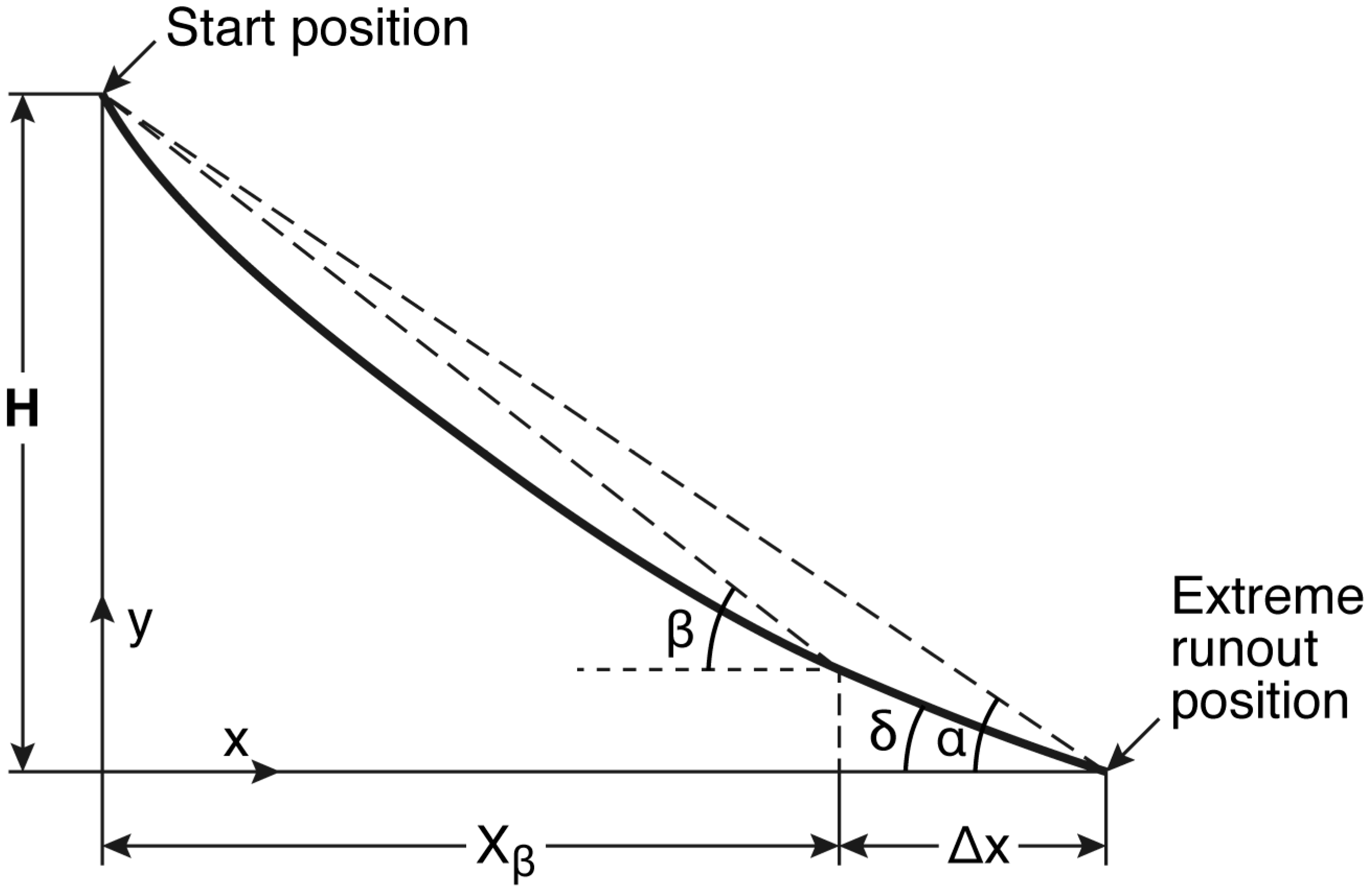
The original dataset from Norway also contained $\delta$ angles defined by a sighting from the $\alpha$ point (extreme runout position) to the $\beta$ point. In [23], a runout ratio $(RR)$ was defined from the three angles as follows:

$$RR={\displaystyle \frac{\Delta x}{X_{\beta }}}={\displaystyle \frac{\tan \beta -\tan \alpha }{\tan \alpha -\tan \delta }}$$

(1)

where $\Delta x$ is the horizontal reach (m) from the $\beta$ point to the extreme runout position, which I term the runout distance (m), and $X_{\beta }$ is the horizontal reach (m) from the start position to the $\beta$ point. The values of $RR$ or $\Delta x$ may take positive or negative values depending on whether the extreme runout position is below or above the $\beta$ point, respectively. If the extreme runout position is at the $\beta$ point, $RR=\Delta x=0$. In Equation (1), the values of $\delta$ take positive values for runout proceeding downslope and negative values for runout on adverse slopes proceeding upslope. Figure 1 contains the geometry with $H$ as the total vertical drop (m) and definitions of all data used in the paper.

The proper collection of field data and application to this problem implies some assumptions. In addition, the selection of a suitable probability distribution to represent the data herein implies some assumptions. The basic assumptions of the method are included in the online Supplementary Material.

3. Results: Description of Data and Descriptive Statistics

Descriptive statistics for the individual datasets reveal important characteristics defining the differences between the datasets. All nine datasets were collected in the field by locating the extreme position recorded for avalanche reach or from vegetative damage assessed in the field. All data have been reported and described in previous publications and in the Supplementary Material. The data descriptions, including recent revisions to the databases and comments on data accuracy, are summarized in the online Supplementary Material.

Table 1. Descriptive statistics (median values) for 9 datasets. The subscript m denotes median values, and N is the number of avalanche events and paths. For each RANGE, an abbreviation is given in parentheses, which is used in the figures below. The data from Norway included only values of the RR, with the remainder of the data noted as N/A: not available.

RANGE	N	$\Delta {\mathit{x}}_{\mathit{m}}(\mathit{m})$	$\mathit{R}{\mathit{R}}_{\mathit{m}}$	${\mathit{X}}_{\mathit{\beta }(\mathit{m})}(\mathit{m})$	${\mathit{H}}_{\mathit{m}}(\mathit{m})$
COLORADO (CO)	130	290	0.32	935	550
ALASKA (AK)	51	260	0.20	1370	730
SIERRA (SI)	90	295	0.43	725	360
AUSTRIA (AU)	79	210	0.13	1700	1110
NORWAY (NO)	127	N/A	0.17	N/A	N/A
ICELAND (IL)	45	175	0.17	1110	575
CANADA (CA)	124	140	0.10	1480	855
SHORT SLOPE (SS)	47	10	0.018	460	225
FOREST (FR)	45	−135	−0.15	890	500

contains the basic data on the median values of $RR$, $\Delta x$, and the following scale parameters $X_{\beta };H$.

For all the values in Table 1, median values are given since they account for the skewness in the data. In [15], the average values were listed for five ranges; however, median values are superior if there is skewness in the data, as is the case here.

In Table 1, the first seven datasets were collected without restriction on scale variables: $X_{\beta },H$. The avalanches had an average return period of about 100 years. The SHORT SLOPE database was restricted to paths with $H\le 350 \mathrm{m}$ and had an estimated average return period of about 50 years [8]. The FOREST dataset contained paths where mature forest cover was penetrated by large avalanches with no estimated average return period assigned [24]. All nine databases have been previously published. An updated description of all the databases is given in the online Supplementary Material.

All the calculated median values concerning distance in Table 1 were rounded to the nearest 5 m distance. Similarly, the $\alpha ,\beta ,\delta$ angles used in calculations were considered to be accurate to the nearest degree. Even without modeling, the median runout distances are of use. A median value would typically apply to an exceedance probability of 0.5, meaning about 50% of extreme avalanches in a database would be expected to run further.

Exploratory data analysis of the individual databases showed that the data skewness ($G_1$) gave a very good explanation of the differences, and it is related to the shape factors of the distributions. We show below (Figure 2 and Figure 3) that either the data sample skewness or the population skewness is an important parameter to explain the differences between $\Delta x$ in the datasets. The data skewness (or sample skewness) is defined as follows:

$$G_1={\displaystyle \frac{\sqrt{N(N-1)}}{N-2}}\left[{\displaystyle \frac{\frac{1}{N}{\displaystyle \sum _{i=1}^N{(R{R}_i-R{R}_{mean})}^3}}{{\left(\frac{1}{N}{\displaystyle \sum _{i=1}^N{\left(R{R}_i-R{R}_{mean}\right)}^2}\right)}^{\frac{3}{2}}}}\right]$$

where $N$ is the sample size and $R{R}_{mean}$ is the mean value of the data. The population or distribution skewness is defined as follows:

$${\gamma }_1={\displaystyle \frac{E\left[{\left(RR-Mean\right)}^3\right]}{{\left(E\left[{\left(RR-Mean\right)}^2\right]\right)}^{\frac{3}{2}}}}$$

where $E$ is the expectation operator, $RR$ is a random variable, and $Mean$ is the distribution mean. In this paper, the random variable is the runout ratio $RR$ with sample values $R{R}_i$.

Figure 2 shows the median runout distance, $\Delta x(m)$, plotted against $G_1$ for eight databases. The data from NORWAY did not include runout distances.

A 95% confidence ellipse is shown. A confidence ellipse is a visual display of the correlation between the variables. The 95% confidence ellipse represents a 95% chance of the next datum falling within the ellipse.

The equation of the regression line is $\Delta x_m=69+165G_1$, with $R^2=0.87; \mathrm{S}.\mathrm{E}. = 55 \mathrm{m}$. The regression line illustrates a very good fit in spite of eight diverse datasets. The data from Norway did not include values of $\Delta x$; therefore, they are not included in the calculations.

Figure 2 is important since it is independent of any probability distribution, and it suggests that any attempt to fit all the databases with a single distribution, as in this study, should include a consideration of data skewness, which is normally related to a distribution shape factor. Since the sample skewness values $(G_1)$ take positive and negative values, so too should the shape factor. Some of the 65 distributions we tested in the next sections had shape factors that took only values (such as the three-parameter gamma distribution); however, they gave poor fits to our databases with low or negative skewness.

Figure 2 and Figure 3 show the relationship between median runout distance $(\Delta x_m)$ and $G_1,k$ (distribution shape factor) for the GLO distribution as an example. Figure 2 is entirely based on data, independent of any distribution, whereas Figure 3 is based on modelling. Figure 2 and Figure 3 show that the median runout distance depends strongly on data skewness or shape factor. The more the data are skewed to the right, the longer the median runout distance, since more cases are running past the $\beta$ reference point.

Figure 3 represents 611 extreme runout distances, and the regression line has $R^2=0.95; \mathrm{S}.\mathrm{E}.= 34 \mathrm{m}$. The equation of the regression line in Figure 2 is $\Delta x_m=67+858k$. A 95% confidence ellipse is shown.

The data skewness ($RR$) is a function of the shape parameter only for the GLO. Linear regression for the relation between $G_1$ and k gave $G_1=4.73k$; $R^2=0.96; \mathrm{S}.\mathrm{E}.= 0.15$. The constant in the regression equation was not statistically significant. The combined results of Figure 2 and Figure 3, along with the $G_1,k$ relation, suggest that the shape parameter $(k)$ of the GLO distribution fitted to the avalanche data is an index of the data skewness and population skewness, and it is importantly related to $\Delta x_m$. For the GEV distribution, calculations gave $\Delta x_m=219+496k; R^2=0.97; \mathrm{S}.\mathrm{E} =24m;$ $G1=0.87+2.73k; R^2=0.90; S.E.=0.26$, where $k$ is the shape parameter for the GEV distribution.

4. Application of the $\mathit{R}\mathit{R}$ Method and Results

In this paper, the $RR$ method is used. Here, the dimensionless $RR$ parameter was fit to 65 different distributions using several large statistics packages. The goal was to assess commonality among the diverse set of databases in this study by seeking single distributions that provided a good fit to all the datasets. The list of distributions, along with the number of parameters for each, is given in the online Supplementary Material. Descriptions and definitions of the distributions may be found in textbooks.

In practice, compiling the databases requires field experience with avalanches. One must be confident that for a path in question the extreme position reached by avalanches can be located either from published reports or in the field and for rough return periods of 100 years or more. Otherwise, the path in question should not be used. Typically, in field work, about 1–2 paths might be included in a full day in the field. In the field, the uncertainty in locating the extreme position by vegetation damage or other evidence at the site is no better than $\pm 10 \mathrm{m}$. The map scale should be 1:10,000 or better, which applies to the data here.

Methods to estimate return periods, including information from this paper, are given in [10,11,25] and in combination with avalanche dynamics in [4,5,6,7,8,26]. The determination of return periods is beyond the scope of this paper, which is exclusively concerned with the empirical, probabilistic prediction of extreme runout of flowing avalanches, meaning those with a dense core of material at the base. The prediction of low-density powder snow avalanche cloud reach is not included in this paper.

We made calculations for 65 distributions for each dataset, but our data include $RR$ with positive and negative values. Therefore, distributions that apply only to positive values of $RR$ were eliminated since no fit could be found for our databases with negative values. In addition, distributions without a shape factor to account for varying data skewness, as in Figure 2, were eliminated. Since the data were collected as extreme cases, one might logically expect to consider extreme value distributions. Gumbel [27] gave three extreme value distributions for which distributions converge to on the tails: Gumbel, Fréchet, and Weibull. Of these, the Fréchet and Weibull apply to positive data values only, and the Gumbel has constant distribution skewness; therefore, all three could be eliminated for application to all nine of our databases.

Previous studies, e.g., [15,20,28] have used only one goodness-of-fit criterion to gauge suitability for comparing datasets: the coefficient of variation $(R^2)$ of probability plots and, mainly, the Gumbel distribution. In this study, we used five goodness-of-fit tests and, in addition, we considered behavior on the tail since the latter is important in engineering decisions. Even though the goodness of fit for distributions may be comparable, engineering decisions normally require the use of a distribution with a heavier tail such that computed runout distances are not too short.

The goodness-of-fit tests used were the Kolmogorov–Smirnov (K-S) test, the chi-squared (C-S) test, both described in [29] (pp. 533–538), and the Anderson–Darling (A-D) test [30]. For the chi-squared test, 4–7 degrees of freedom and equal probabilities for bins were used. In addition, probability (PP) and quantile (QQ) plots were made to assess the distribution fits overall. A PP plot is used to compare an empirical CDF with the theoretical CDF of the distribution. A QQ plot is used to compare quantiles of the data with the quantiles of the theoretical distribution.

For the (K-S) and (C-S) tests, the statistical significance level $({\alpha }_s)$ was used to gauge goodness of fit. It represents the probability of rejecting a fitted distribution when the data fit the distribution well. The quantity $(1-{\alpha }_S)$ is similar to a confidence level. The lower the value of $1-{\alpha }_s$, the more stringent the goodness-of-fit requirement and the lower the critical value of the goodness-of-fit statistic. The most commonly used values for ${\alpha }_s$ are typically 0.1 and 0.05; however, here, the more stringent value of 0.2 has been used. For all distributions, the critical value was determined for ${\alpha }_s=0.2,0.1,0.05,0.02,0.01$, and the calculated value of the statistic was compared with the critical value for hypothesis testing against the null hypothesis that the distribution considered was a good fit. The null hypothesis was that the distribution was not rejected if the calculated value from the data was less than the critical value.

For the (A-D) test, goodness-of-fit was partly assessed by ensuring that the test statistic had a low value in comparison with the other distributions. The (A-D) statistic was calculated for all the fitted distributions with ranks provided. For the (A-D) statistic, the critical values depend on the distribution, the sample size, and the shape parameter. The critical values as a function of ${\alpha }_s$ are not known for many of the distributions. Multiple regression analyses were provided in [31] for extreme value distributions including the GLO and GEV distributions as a function of ${\alpha }_s$, sample size, and shape parameter. In

Table 2. Goodness-of-fit statistics for (K-S) and (C-S) critical values in parentheses for the statistical significance parameter: ${\alpha }_s=0.2$. The distribution parameters are denoted $(k,\sigma ,\mu )$ as follows: shape, scale, and location parameters. The goodness-of-fit statistics are labelled as follows: K-S: Kolmogorov–Smirnov; A-D: Anderson–Darling; C-S: chi-squared. For the A-D statistic, the critical value of ${\alpha }_s$ at which the test passed is listed in parentheses.

RANGE	$\mathbf{K}\text{-}\mathbf{S} ({\mathit{\alpha }}_{\mathit{s}}=0.2)$	$\mathbf{A}\text{-}\mathbf{D} ({\mathit{\alpha }}_{\mathit{S}})$	$\mathbf{C}\text{-}\mathbf{S} ({\mathit{\alpha }}_{\mathit{s}}=0.2)$	$\mathit{k}$	$\mathit{\sigma }$	$\mathit{\mu }$
GLO GEV (COLORADO)	0.06 (0.09) 0.05 (0.09)	0.61 (0.05) 0.38 (0.20)	13.10 (9.80) * 12.84 (9.80) *	0.29 0.18	0.12 0.16	0.34 0.28
GLO GEV (ALASKA)	0.13 (0.15) 0.12 (0.15)	0.55 (0.05) 0.40 (0.10)	5.26 (7.29) 4.12 (7.29)	0.27 0.15	0.07 0.09	0.21 0.18
GLO GEV (SIERRA)	0.08 (0.11) 0.08 (0.11)	0.73 (0.01) 0.54 (0.01)	5.88 (8.56) 5.49 (8.56)	0.24 0.10	0.13 0.18	0.44 0.36
GLO GEV (AUSTRIA)	0.08 (0.12) 0.07 (0.12)	0.51 (0.05) 0.39 (0.10)	6.28 (8.56) 6.76 (8.56)	0.23 0.08	0.05 0.07	0.12 0.09
GLO GEV (NORWAY)	0.07 (0.10) 0.05 (0.10)	0.51 (0.05) 0.29 (0.20)	4.39 (8.56) 4.03 (8.56)	0.11 −0.10	0.06 0.10	0.17 0.13
GLO GEV (ICELAND)	0.14 (0.16) 0.12 (0.16)	0.78 (0.01) ** 0.56 (0.05)	5.96 (5.99) 2.89 (5.99)	0.08 −0.14	0.08 0.14	0.17 0.12
GLO GEV (CANADA)	0.07 (0.10) 0.09 (0.10)	0.64 (0.01) 0.90 (<0.01)	7.22 (8.56) 15.89 (8.56) *	0.07 −0.16	0.05 0.09	0.11 0.07
GLO GEV (SHORT SLOPE)	0.09 (0.15) 0.09 (0.15)	0.35 (0.20) 0.38 (0.20)	5.21 (5.99) 2.76 (5.99)	−0.07 −0.42	0.16 0.30	0.07 −0.03
GLO GEV (FOREST)	0.09 (0.16) 0.09 (0.16)	0.47 (0.10) 4.31 (<0.01) *	3.44 (5.99) N/F **	−0.20 −0.69	0.08 0.18	−0.15 −0.20

, the (A-D) calculated is provided along with the value of ${\alpha }_s$ by which the test passed from the critical values provided in [31]. In Table 2, the values of (K-S) and (C-S) represent comparison with critical values for ${\alpha }_s=0.2$. For a given dataset, the decision about which distribution has a better fit was based primarily on a comparison of the critical values, with the calculated values of the A-Ds. For example, if the critical value for ${\alpha }_s$ was the same, we would consider the fit equivalent; however, if it was higher for a distribution over another, we would say the former would be the better fit. The A-D is very powerful, since it compares cumulative distribution functions over the entire distribution, not just the tail. It is the only one of the goodness-of-fit tests that can discriminate among the distributions to determine the shape of the best-fitting one.

Our considerations for the most important distributions included all five goodness- of-fit tests, plus the behavior on the tails, since the latter is important in engineering decisions. A distribution with a heavier tail is normally favored in engineering applications since others would yield shorter runout distances for the same exceedance probability or return period. The A-D was given the most weight, along with the prediction of a heavier tail.

Below, we have presented detailed calculations on the two best choices (GLO; GEV) to fit all of our databases. Both have shape parameters (positive or negative) to account for data skewness, a location, and a scale parameter. Table 2 contains the goodness-of-fit results and distribution parameters.

Table 2 contains goodness-of-fit statistics and parameters for the nine datasets fit to the GLO and GEV distributions using either Maximum Likelihood Estimates (MLEs) or Method of Moments (MMs) to determine the distribution constants. For the calculations of all 65 distributions, MM was used for distributions where moment estimates are available for all possible parameter values and do not involve iterative numerical methods. Examples include Normal, Log-Normal, Gumbel, Pearson type 3, Log Pearson type 3, and Weibull. The MLE was used for the other distributions requiring numerical methods. The maximum number of MLE iterations used for all calculations was 100, with accuracy ${10}^{-5}$. For example, the shape parameter k for COLORADO was calculated as 0.29275; however, the value presented was 0.29 (Table 2 below).

The data from AUSTRIA included $\Delta x,X_{\beta }$; therefore, it was possible to perform the calculations from the ratio $(\Delta x/X_{\beta })$ directly as well as using the angles. The ratio calculations gave $k=0.24;\sigma =0.06;\mu =0.15$ for comparison with the values above.

In Table 2, entries with * failed the test for the specified values of ${\alpha }_s$ The C-S entries for COLORADO passed at ${\alpha }_s=0.05$. The A-D entry for the GLO for Iceland (**) passed the critical value of the A-D for 0.01. From [31], the critical value for A-D is actually 0.77; however, the calculated value (0.78) is essentially the same, given the uncertainty from the regression expressions. The entry N/F ** for the GEV (FOREST), C-S, signifies that no fit was found for the calculations.

If the critical value of the A-D is chosen as ${\alpha }_s=0.01$, and all databases pass for the GLO, whereas the GEV fails for two. If the critical value of A-D is chosen as ${\alpha }_s=0.05$, then the GLO fails for three databases, and the GEV for three.

Of the 65 distributions tested, only five had a shape factor that could take positive and negative values: the GEV and GLO, which have three parameters (shape, scale, location), and three four-parameter distributions, as follows: generalized gamma, Johnson SB, and Johnson SU. No fit was obtained for seven databases for the Johnson SU. For Johnson SB, three databases failed both the A-D and C-S tests, and for the generalized gamma, three databases failed both the A-D and C-S, with another failing the C-S.

It was stated above that the three classical extreme value distributions will not provide fits for all the databases. Two other extreme value distributions were considered: the three-parameter Weibull distribution and the three-parameter Fréchet distribution. Both have a shape factor, a scale, and a location parameter so that negative values may be accepted. The three-parameter Fréchet distribution gave erroneous, unrealistic results on the tail of the distribution for six of the nine databases. The Weibull three-parameter distribution had a lighter tail than either of the two distributions in Table 2. Both are restricted to positive shape factors, as with the three-parameter gamma distribution.

We tested all 65 of the distributions (Supplementary Material), and the two highlighted distributions were the best concerning our considerations, which were extreme behavior on the tail and goodness of fit. The four, five, and six-parameter distributions (Beta, Burr, Dagum, generalized gamma, JohnsonSB, JohnsonSU, Pearson6, Phased Bi-Exponential4, Wakeby 5, Phase Bi-Weibull 6) all had either light tails compared to, e.g., the GLO (

Table 3. Calculations of the $RR$ for exceedance probabilities Pe: 0.01 and 0.005 (or spatial return period 100 and 200) for the two highlighted distributions: generalized logistic (GLO) and generalized extreme value (GEV).

Pe →/ RANGE ↓	GLO	GLO	GEV	GEV
Pe →	0.01	0.005	0.01	0.005
CO ↓	1.48	1.83	1.43	1.71
AK	0.85	1.02	0.78	0.94
SI	1.51	1.78	1.41	1.62
AU	0.53	0.64	0.48	0.56
NO	0.54	0.60	0.50	0.54
IL	0.62	0.70	0.59	0.64
CA	0.38	0.45	0.36	0.39
SS	0.70	0.77	0.58	0.61
FR	0.09	0.12	0.05	0.05

), very high A-D statistics combined with two-shape parameters, or wildly varying distribution parameters (up to ${10}^6$). The other three-parameter distributions (Erlang3, Error3, Log-Pearson 3, Log Logistic 3, Power Function 3, Triangular) had either very high A-D statistics, wildly varying distribution parameters (up ${10}^8$), and wildly varying results on the tails. In [28], the Generalized Pareto distribution was fit to two truncated datasets. The Generalized Pareto failed the goodness-of-fit tests for all our distributions since it only applies to truncated datasets. The truncation of a dataset changes the exceedance probability for events on the tail of the distribution.

We cannot rule out that some other distribution other than the 65 analyzed might be found, which matches our criteria better than the two highlighted (GLO and GEV). However, we believe the two highlighted sets give a very good picture of the meaning of our nine databases.

5. Description of the GLO and GEV Distributions

The pdf (probability density function) of the GLO distribution is given in Equation (2).

$$f(RR;k,\sigma ,\mu )={\displaystyle \frac{{\left(1+\frac{k(RR-\mu )}{\sigma }\right)}^{-(1/k+1)}}{\sigma {\left[1+{\left(1+\frac{k(RR-\mu )}{\sigma }\right)}^{-1/k}\right]}^2}}$$

(2)

where $(k,\sigma ,\mu )$ are the shape factor, scale factor ($\sigma$ > 0), and location parameter, respectively. The shape factor $(k)$ lies between $[-1,1]$ when the pdf is bounded, and for the data here, it is in the range [−0.20, 0.29]. Reversing the sign of $k$ reflects the pdf function about $RR=\mu$: the median value. This is a very important property for the datasets here since $k$ takes positive and negative values, which imply positive and negative skewness for the distribution and sample values. We showed above that the data skewness, which is related to $k$, is the key to understanding the differences in the median runout distance.

The GLO distribution has previously been used in flood frequency/stream flow analysis [32,33,34] and rainfall analysis [31].

The cumulative distribution function (CDF) for the GLO distribution is as follows:

$$F(RR;k,\sigma ,\mu )={\displaystyle \frac{1}{1+{\left(1+\frac{k(RR-\mu )}{\sigma }\right)}^{-1/k}}}$$

(3)

For $k>0$, the domain is $RR>\mu -\sigma /k$ and for $k<0$, it is $RR<\mu -\sigma /k$. After considerable algebra, it can be shown from [35] that for $k>0$, $f(RR)$ converges to a Weibull distribution on the left tail (smallest values) and a Gumbel distribution on the right tail (largest values). When $k=0$, it becomes the logistic distribution. Similarly, for $k<0$, $f(RR)$ converges to a Gumbel distribution on the left tail (smallest values) and a Weibull distribution on the right tail. When $\mu =\sigma /k$, the GLO (shifted log-logistic) distribution reduces to the log-logistic distribution; however, the latter applies only to positive values of RR.

The exceedance probability is given by $p_e(RR;k,\sigma ,\mu )=1-F(RR;k,\sigma ,\mu )$.

The pdf of the GEV distribution is given by the following:

$$f(RR,k,\sigma ,\mu )={\displaystyle \frac{1}{\sigma }}\exp {\left(-(1+kz\right)}^{-1/k}){(1+kz)}^{-1-1/k}$$

(4)

where $z=(RR-\mu )/\sigma$. The CDF is given by the following:

$$F(RR,k,\sigma ,\mu )=\exp \left(-{(1+kz)}^{-1/k}\right)$$

(5)

The shape factor ($k$) may take positive and negative values. The value of $k$ governs the behavior of the tail. If $k$ = 0, the behavior is for the Gumbel distribution; if $k$ > 0, it is the Fréchet, and if $k$ < 0, it is the Weibull.

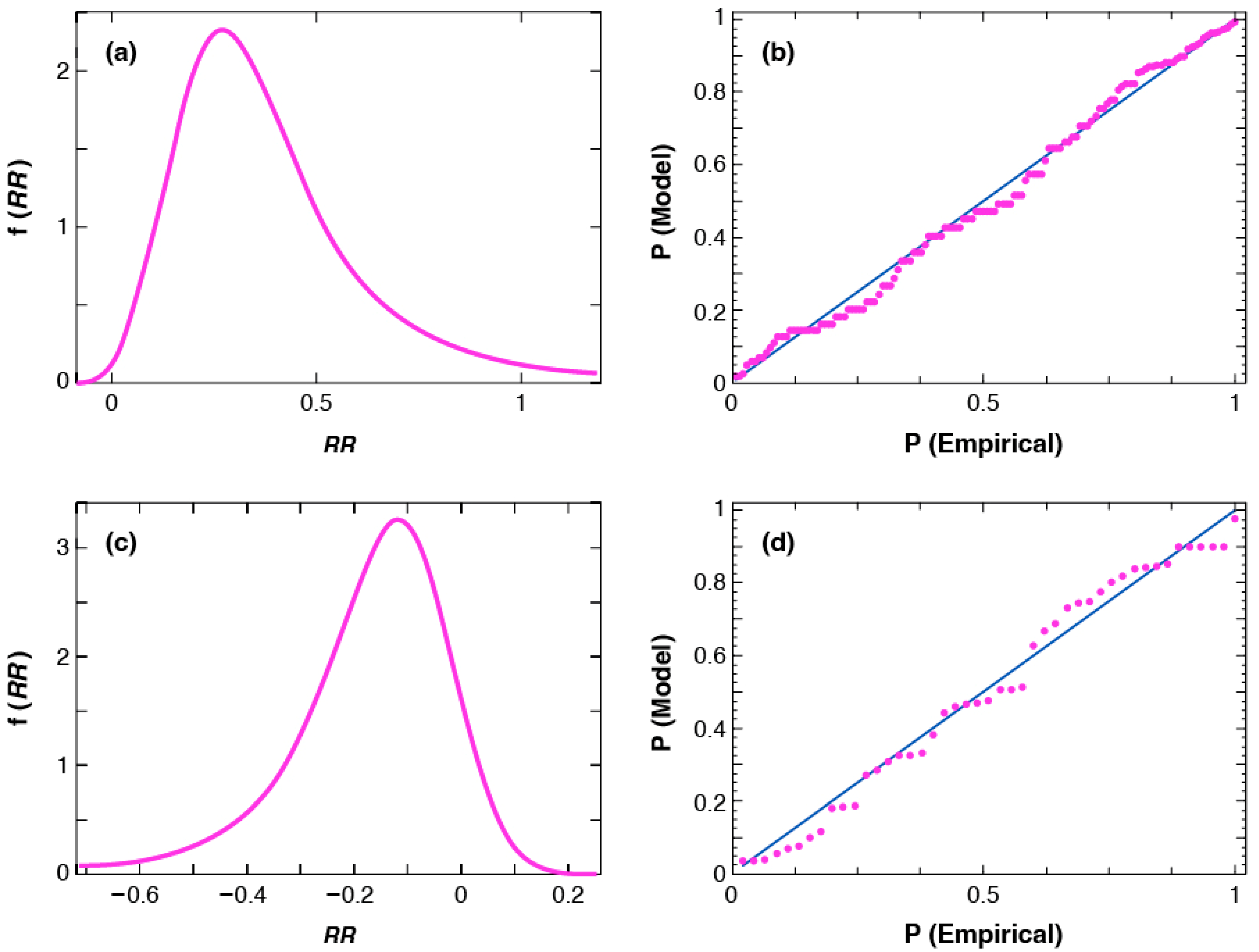
Both the GLO and GEV may be considered as extreme value distributions. The original work on extreme values [27] considered only the Gumbel, Fréchet, and Weibull for convergence on the tails. However, there are a number of distributions [35] that may be considered extreme value distributions. Table 3 and Figure 4 (below) show that, for the extreme avalanche data, the GLO is more extreme compared to the GEV.

Figure 4 shows the pdfs and probability (PP) plots for COLORADO (positive skewness) and FOREST (negative skewness) for the data fit to a GLO distribution.

6. Extremal Behavior on the Tails

Table 3 contains the results for the prediction of $RR$ on the tails for exceedance probabilities 0.01 and 0.005 for the highlighted GLO and GEV distributions. The exceedance probability represents the probability that the position in question will have a runout that reaches or exceeds the location. For example, if the exceedance probability is 0.01, then the 1 in 100 $RR$ in the database would be expected to reach or exceed the location. The 1 in 100 avalanche $RR$, in a database, could also be termed the spatial return period 100, as opposed to a true return period, which involves introducing time. For most of the databases here, there are rough estimates of the range for return periods for the datasets; however, there are very few avalanche paths in the datasets for which the return period has been determined with good accuracy. The results in this paper may be combined with other information at a site to estimate return periods; however, the results in this paper cannot be used alone to estimate return periods [11]. Some practitioners use statistical prediction alone of the spatial return period or exceedance probability.

The GLO distribution has a heavier tail than the GEV for all databases. Figure 5 shows a spatial return period comparison for the two distributions for data from the Sierra Nevada.

The calculations in Table 1 and Table 3 can be used to rank the datasets in terms of extreme median runout distance (Figure 1) and $RR$, respectively. The data from SIERRA and COLORADO represent the most extreme ones in terms of median runout distance (independent of distribution) and $RR$ (for either GLO or GEV).

7. Conclusions and Discussion Summary

1. We presented a rigorous analysis of the world’s largest collection of extreme snow avalanche runout distances $(\Delta x)$ (611) and $RR$ (738). The analysis showed that the data skewness $G_1$ or the distribution shape factors $(k)$ of two highlighted extreme value distributions (GLO and GEV) are key to explaining the differences in either the median runout distance or median $RR$ for the different datasets.

2. The two highlighted distributions were selected based on an analysis of 65 distributions listed in the Supplementary Material. Using five goodness-of-fit tests, we tested all nine of our databases against each distribution to explore commonality among the datasets. Data characteristics required, including needing both positive and negative values of $RR$ and positive and negative values of $G_1$ implying both positive and negative distribution shape factors $(k)$ for the datasets that eliminated many distributions.

3. The descriptive statistics in Table 1 and the distribution constants in Table 2 are immediately useful in comparing our results to other datasets or future datasets. For the six datasets collected without restrictions on total vertical drop (CO, AK, SI, AU, IL, CA), the median runout distance ranges from 140 m to 295 m, representing positions for which about 50% of extreme avalanches would be expected to run further. The distribution constants (Table 2) for the GLO and GEV and the distribution scale factors ($H_m;X_{\beta (m)}$) in Table 1 may be used to compare our results with other datasets collected.

4. Probabilistic engineering decisions depend not only on the goodness of fit but also on the heaviness of the tail of a chosen distribution. Our analysis showed that of the two highlighted distributions, the GLO has the heavier tail. For our data, the GEV predicts shorter runout for the same exceedance probability or spatial return period. The $RR$ method is important in engineering an assessment of the extreme avalanche runout distance since it is completely independent of the other method for runout prediction, which is based on avalanche dynamics. The $RR$ method feeds directly into return period determination [10,11] since return period determination also implies probabilistic methods for the long return periods of an order of 100 years, typically used in planning.

5. Previous results, e.g., [8,9,15,20,36] originate from databases tested against the Gumbel or Generalized Pareto [28] distributions, only with one goodness-of-fit test. The application of the rigorous procedure in this study for the Gumbel distribution showed that five of our nine databases (CO, IL, CA, SS, FR) failed the A-D test with values higher than the critical value at 0.01. All of our databases failed for the Generalized Pareto distribution since it applies to truncated distributions. Truncation changes the exceedance probabilities for events on the tail of a distribution.

6. In regard to climate change, the review in the Supplementary Material suggests that there is no evidence at this time for climate change affecting extreme, rare avalanche events. Extreme avalanches are normally thought to occur by deep weak layers in the snowpack being overloaded, and there is no evidence of that for events occurring on the time scale of on the order of 100 years, which most of the data here apply to. Extreme avalanches are rare, discrete, and independent events with no memory of past events and, as such, may be thought of as Poisson events. The encounter probability $(E_p)$ for Poisson events [37] represents the probability of at least one event reaching or exceeding a position with a return period $(T)$ over the time period of observation $(L)$: $E_p=1-\left(e^{-L/T}\right)$. For the return period $T=100$ years and observation period $L=50-100$ years, the encounter probability ranges from 39 to 63% for observation of at least one of these extreme events. The effects of climate change on average avalanche activity were noticed to begin about 50 years ago [38,39]. We suggest that the most likely adjustments for climate change will be in regard to the exceedance probability used, not the lack of stationarity for extreme databases.