
GS24b and GS24bc Ground Motion Models for Active Crustal Regions Based on a Non-Traditional Modeling Approach

Abstract
1. Introduction
- The global backbone GS24b model that uses the closed-form approximation of the spectral acceleration as a multiplication of the PGA and spectral shape (normalized spectral acceleration spectrum) functions. This model could be used for adjusting to specific ACR regions (e.g., southern and northern California), creating partially non-ergodic models.
- The ergodic model representing the backbone GS24b GMM adjusted for the depth to the shear-wave velocity horizon of 2.5 km/s (), style of faulting () and also for the moment magnitude , time-averaged shear-wave velocity in the upper 30 m and closest distance to the fault rupture residuals.
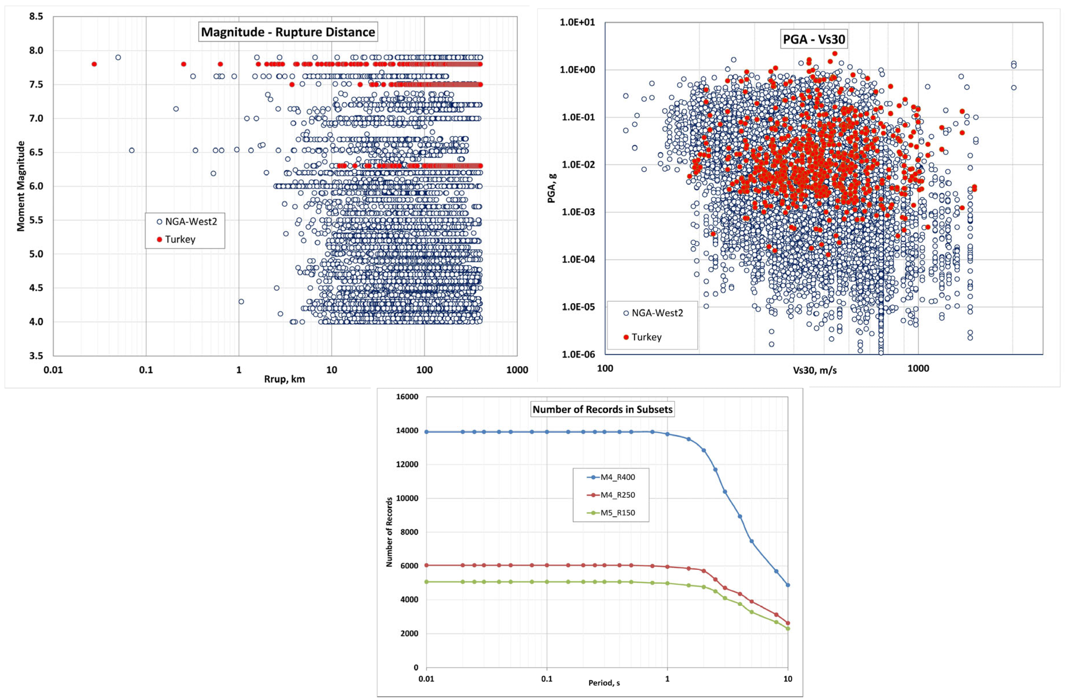
2. Datasets
- The 2nd dataset (subset of the 1st dataset) includes 5063 data points for ≥ 5.0 and ≤ 150 km (called M5_150), and the final dataset:
- The 3rd dataset (also subset of the 1st dataset) includes 6045 data points covering the range of 4 ≤ ≤ 7.9 and ≤ 250 km (called M4_R250).
- 4.0 ≤ < 4.5 and ≤ 25 km
- 4.5 ≤ < 5.0 and ≤ 50 km
- 5.0 ≤ < 5.5 and ≤ 75 km
- 5.5 ≤ < 6.0 and ≤ 100 km
- 6.0 ≤ < 7.0 and ≤ 150 km
- 7.0 ≤ < 7.5 and ≤ 200 km
- 7.5 ≤ ≤ 7.9 and ≤ 250 km
3. GS24b Backbone Ground Motion Model
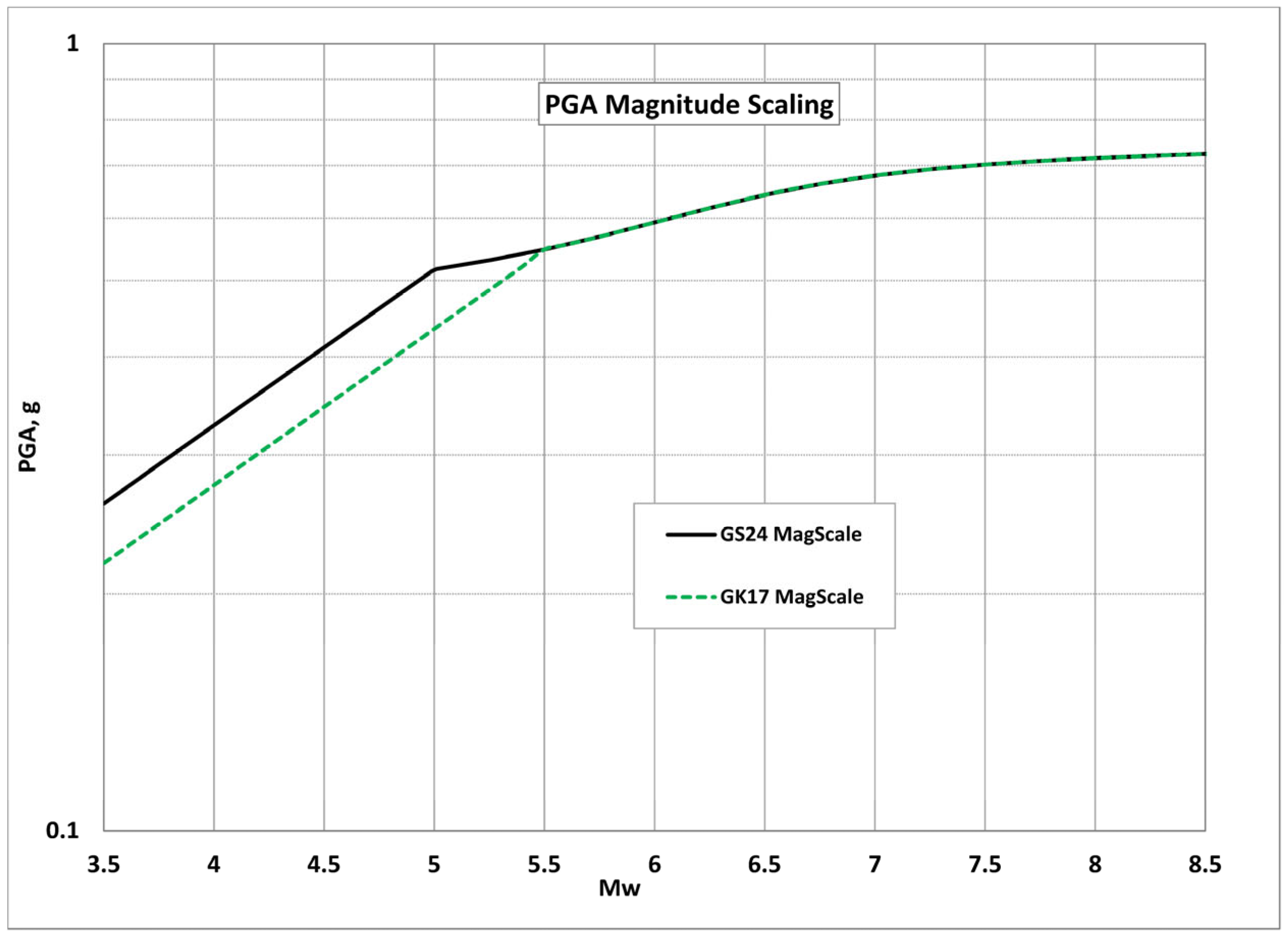
3.1. PGA Scaling
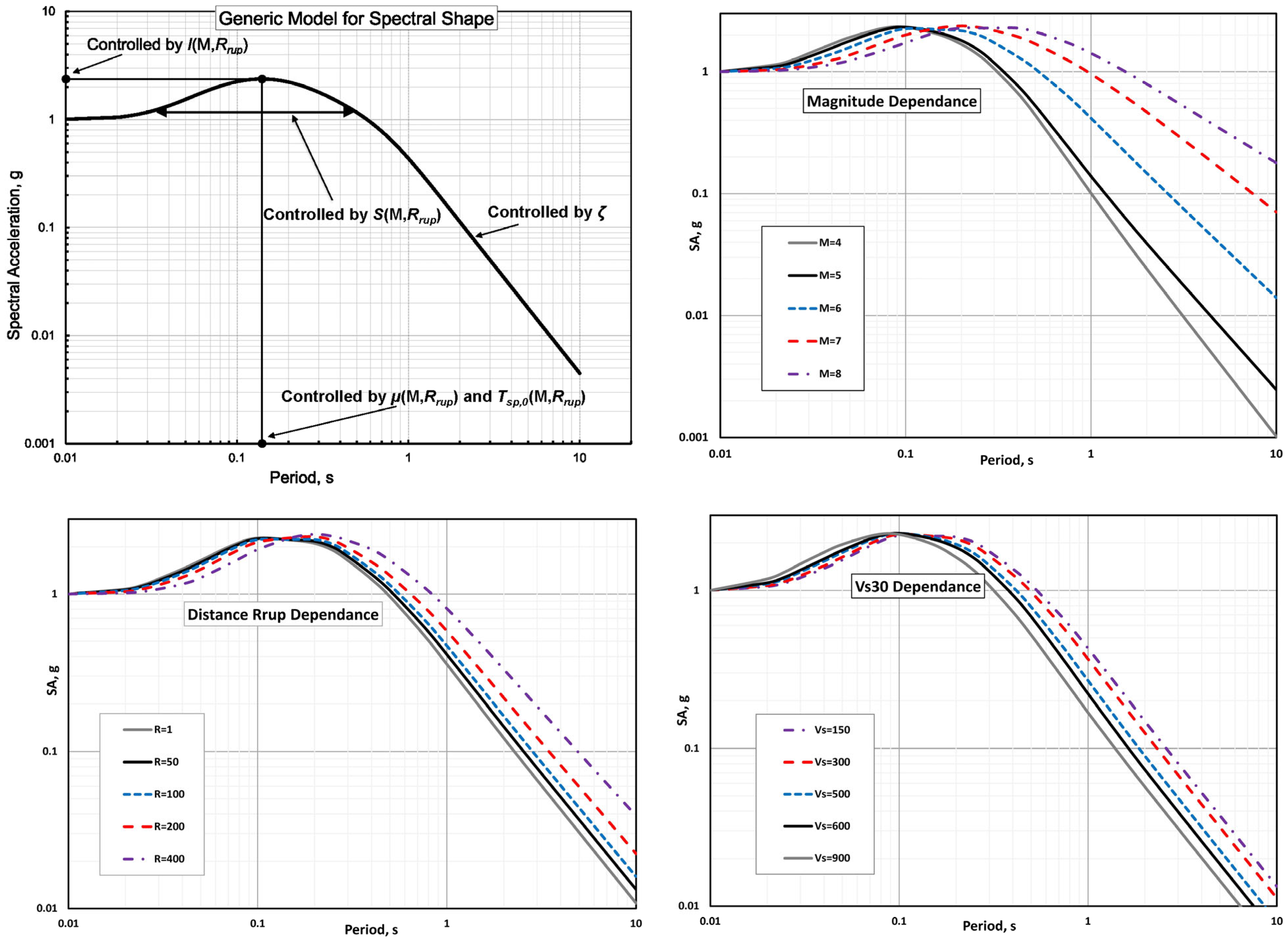
3.2. Spectral Shape Model
4. GS24b Backbone Model
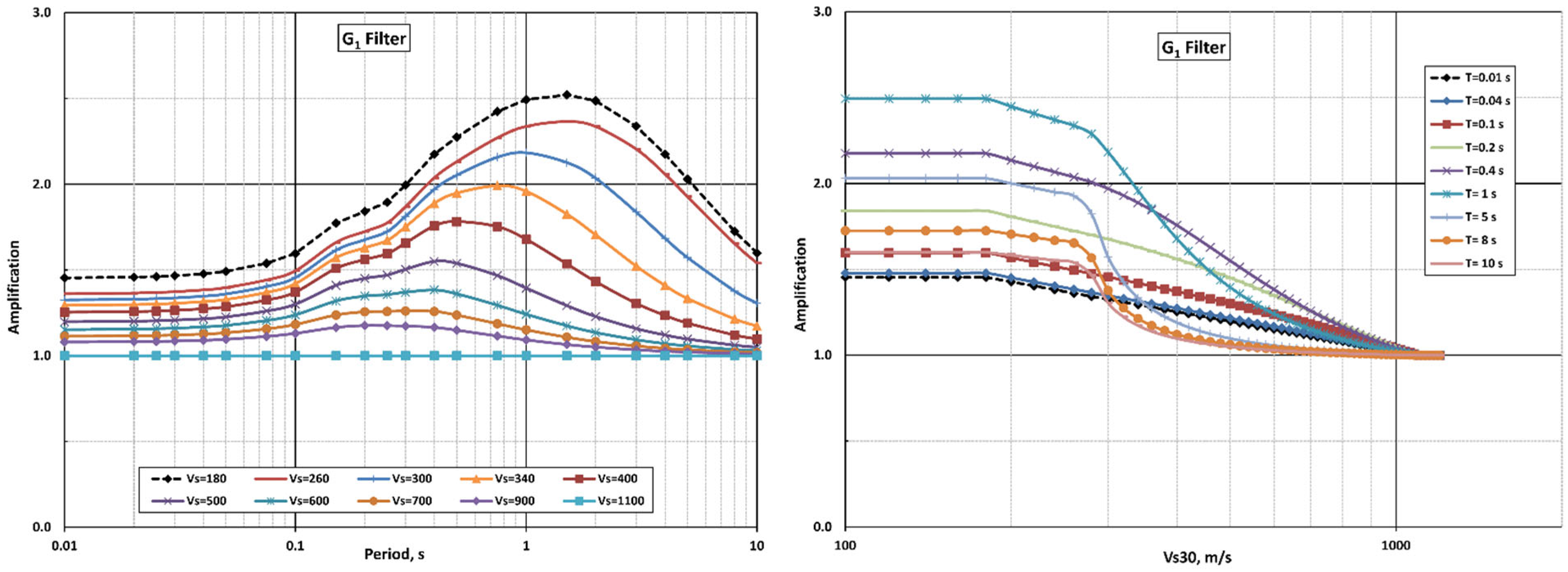
4.1. Site Response Term
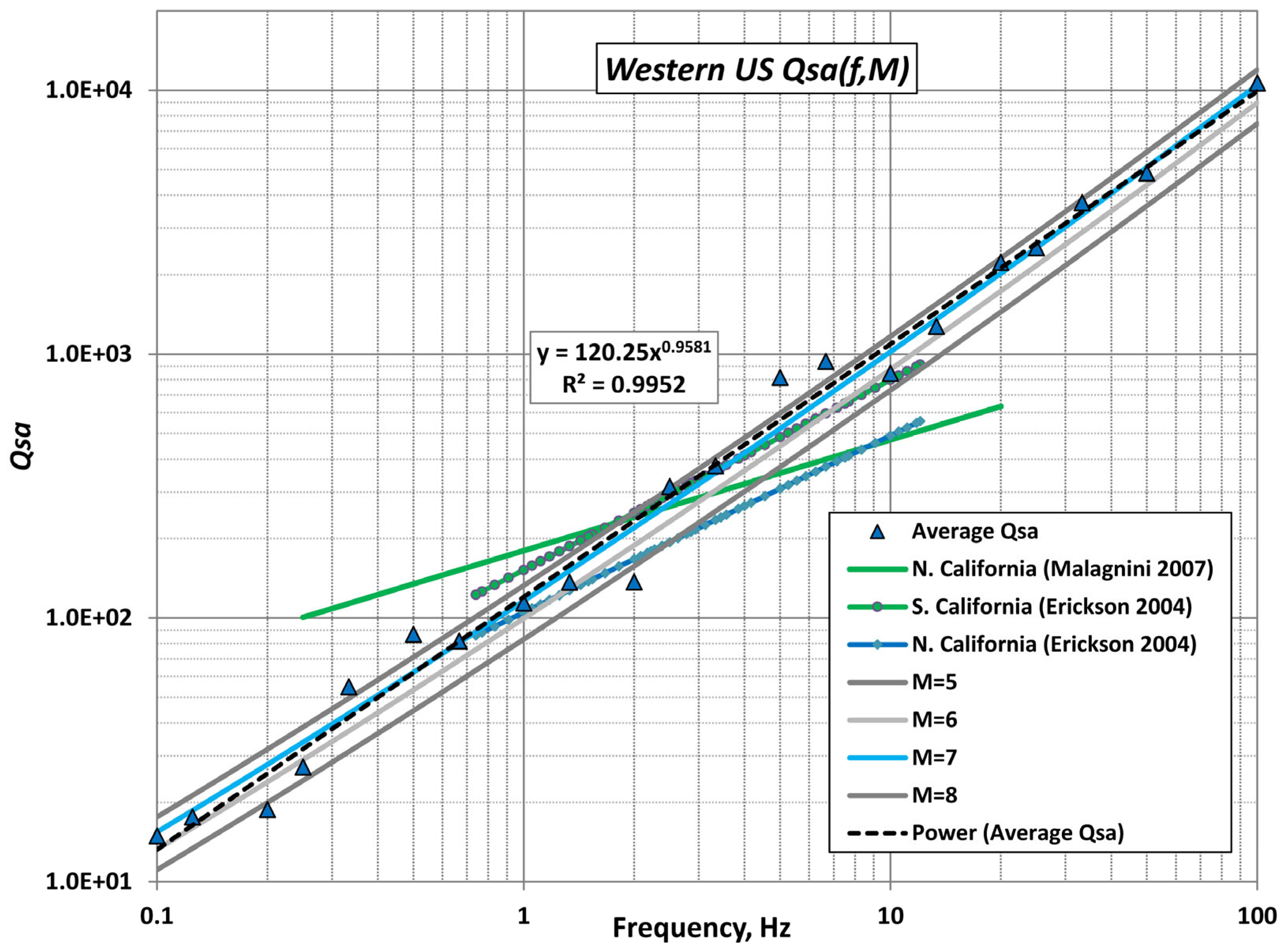
4.2. Apparent Attenuation of Spectral Accelerations
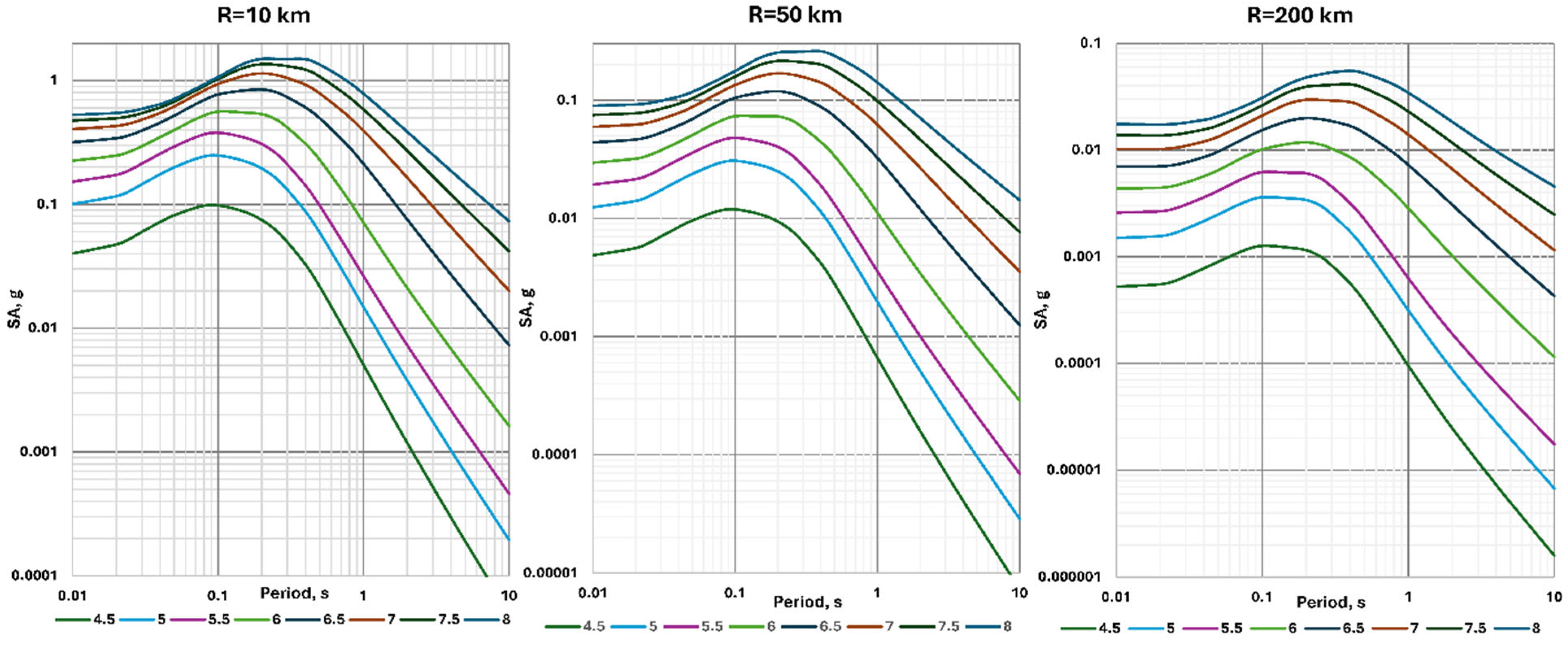
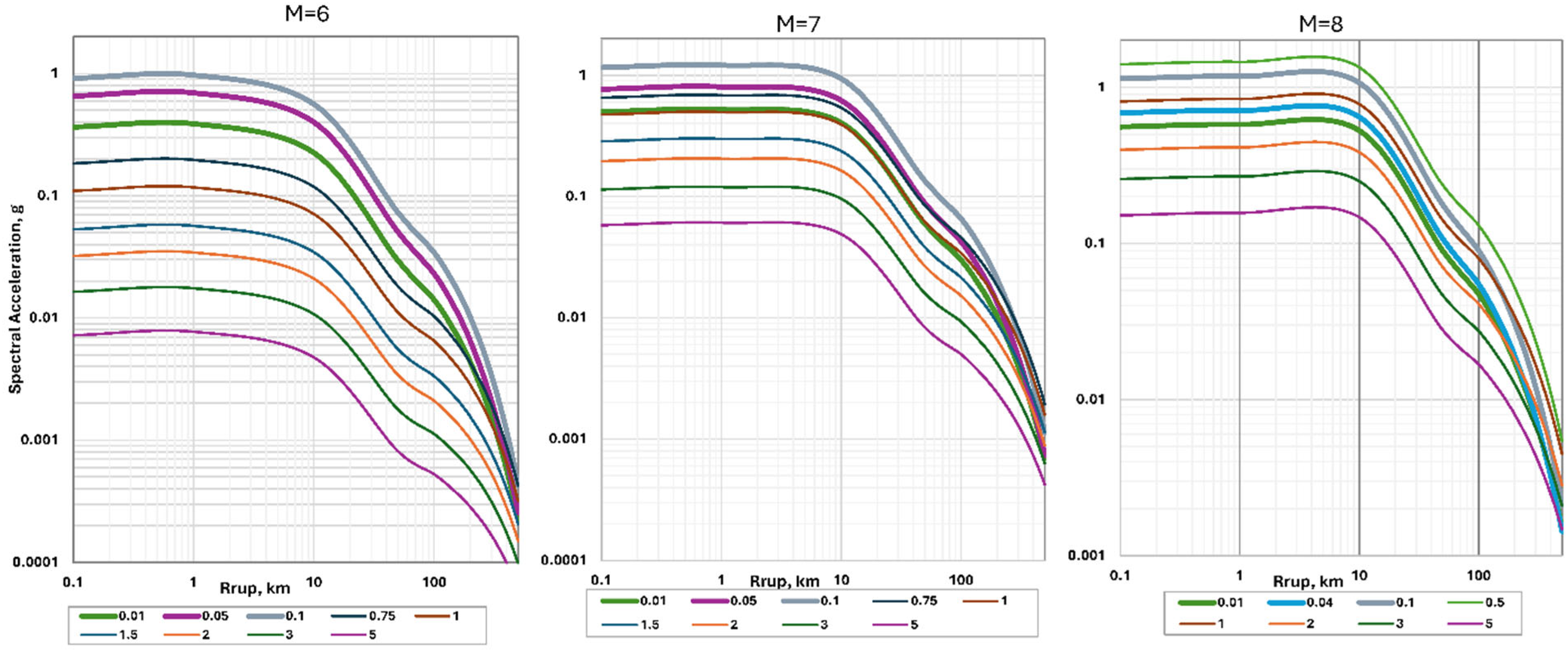
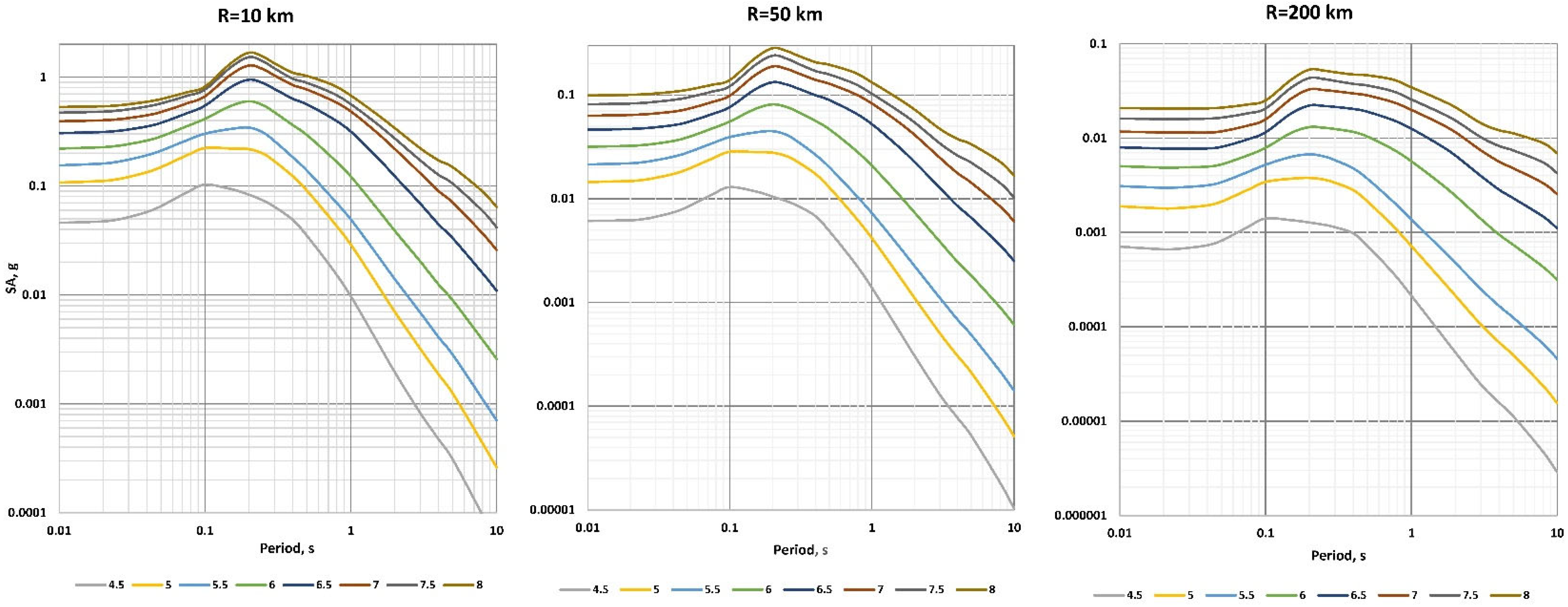
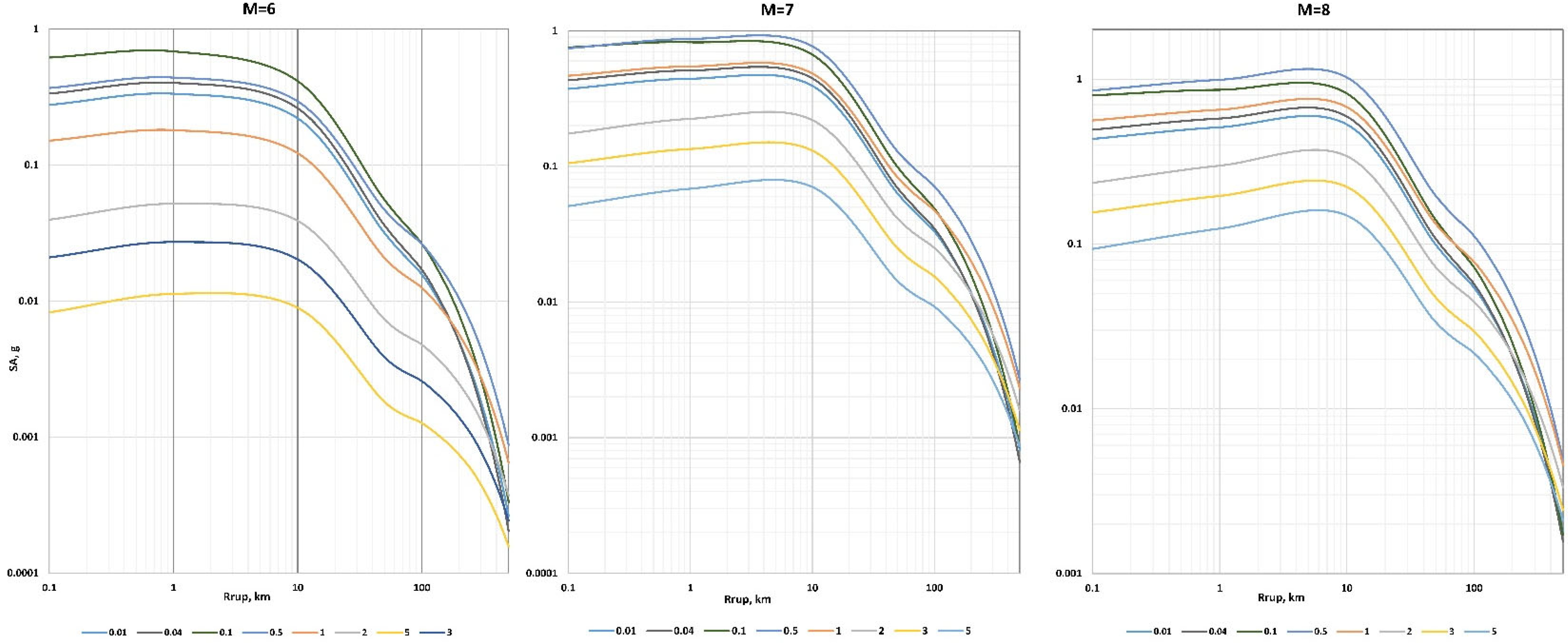
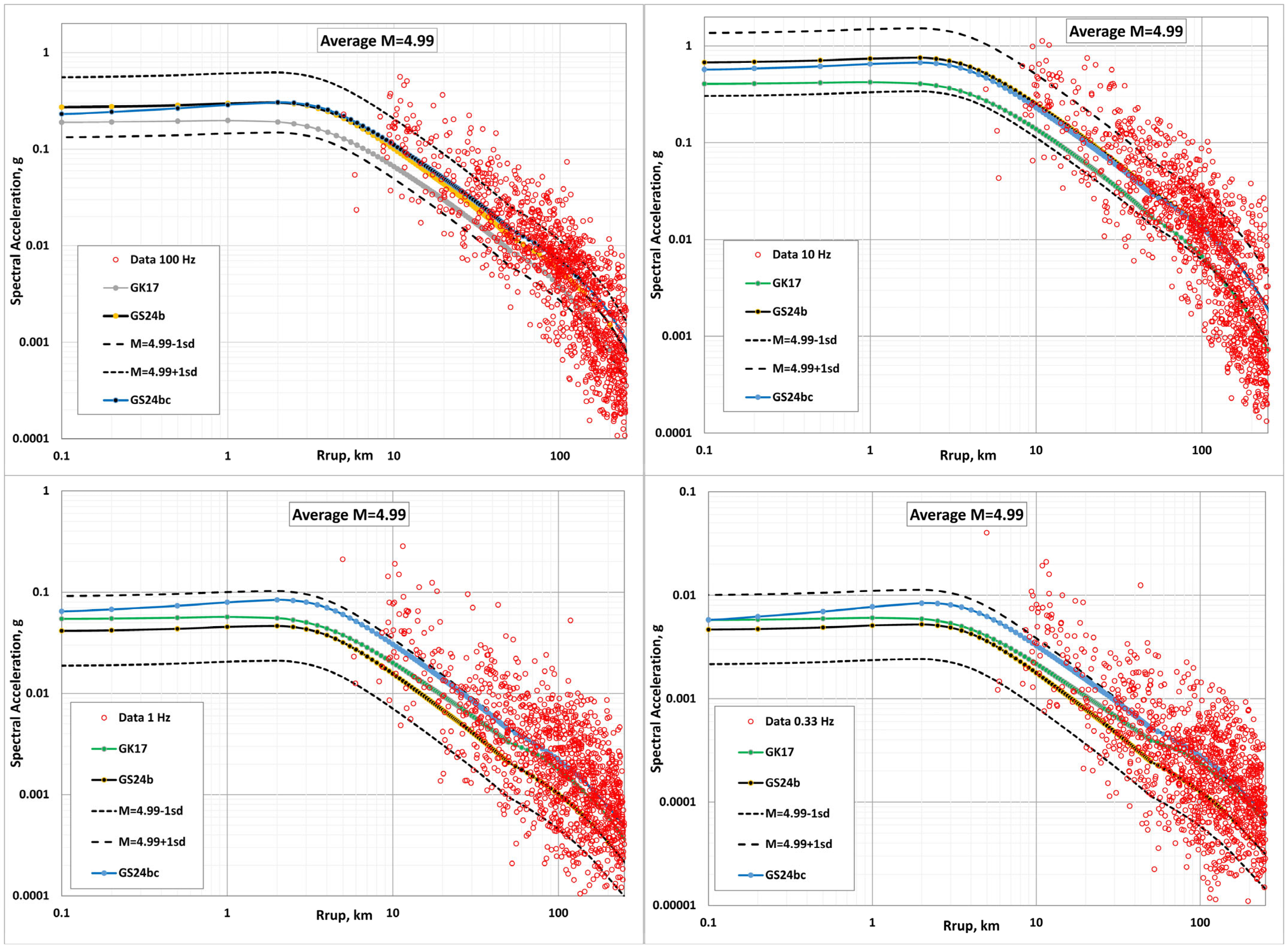
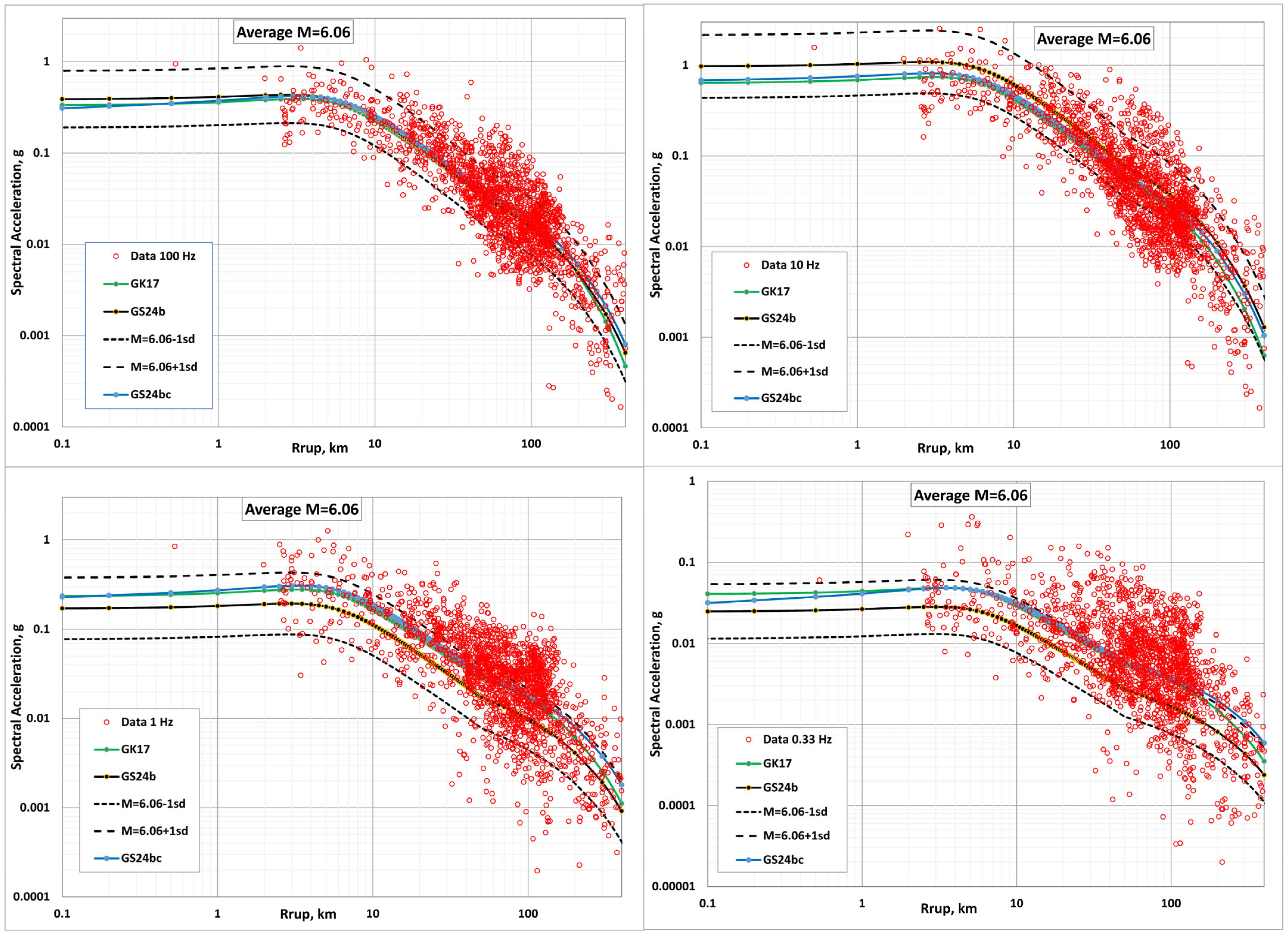
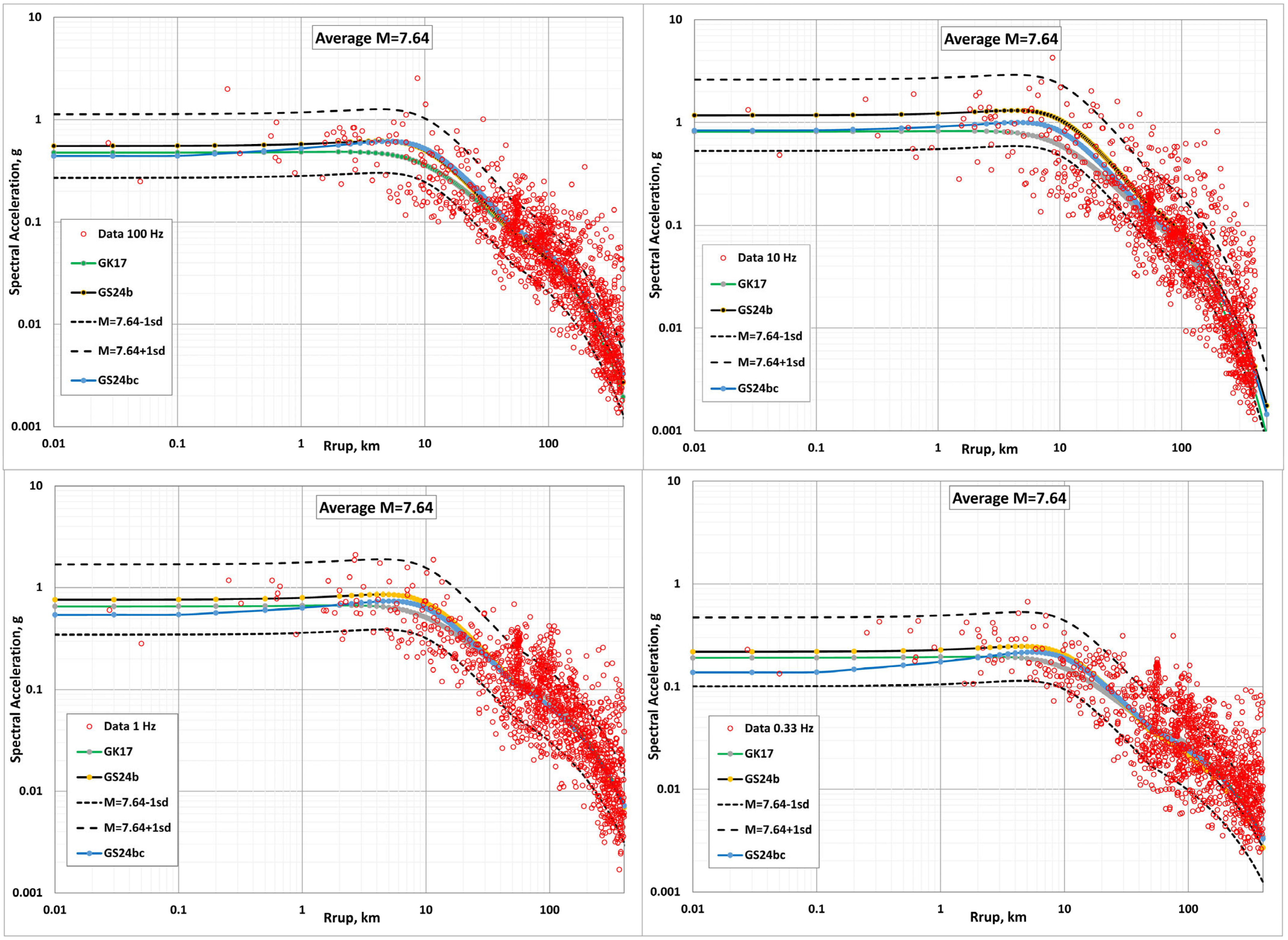
4.3. Examples of Backbone Model
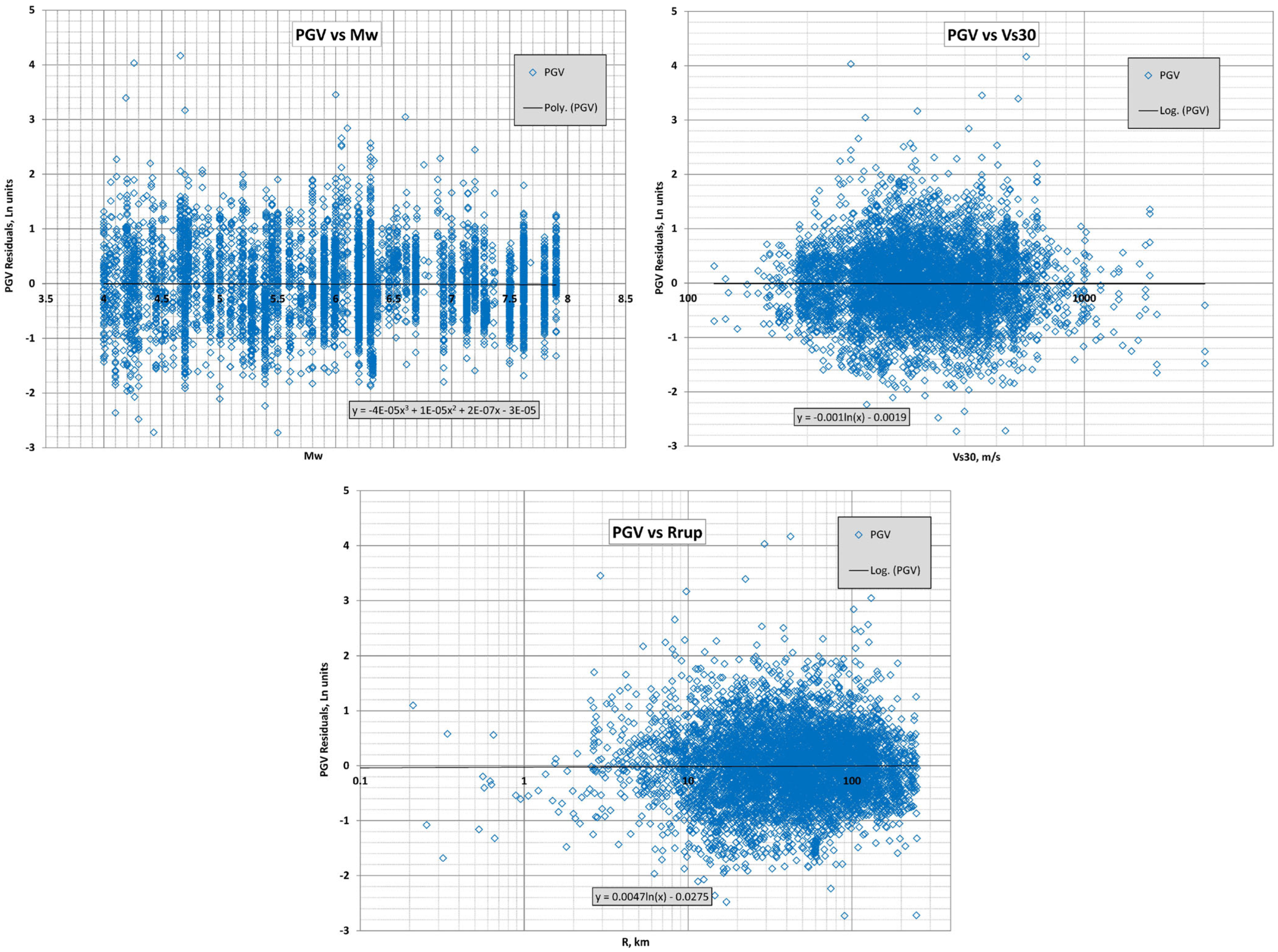
Peak Ground Velocity
4.4. GS24bc Model
- 4.77 ≤ ≤ 5.21 with an average = 4.99
- 5.70 ≤ ≤ 6.24 with an average = 6.06
- 7.28 ≤ ≤ 7.9 with an average = 7.64.
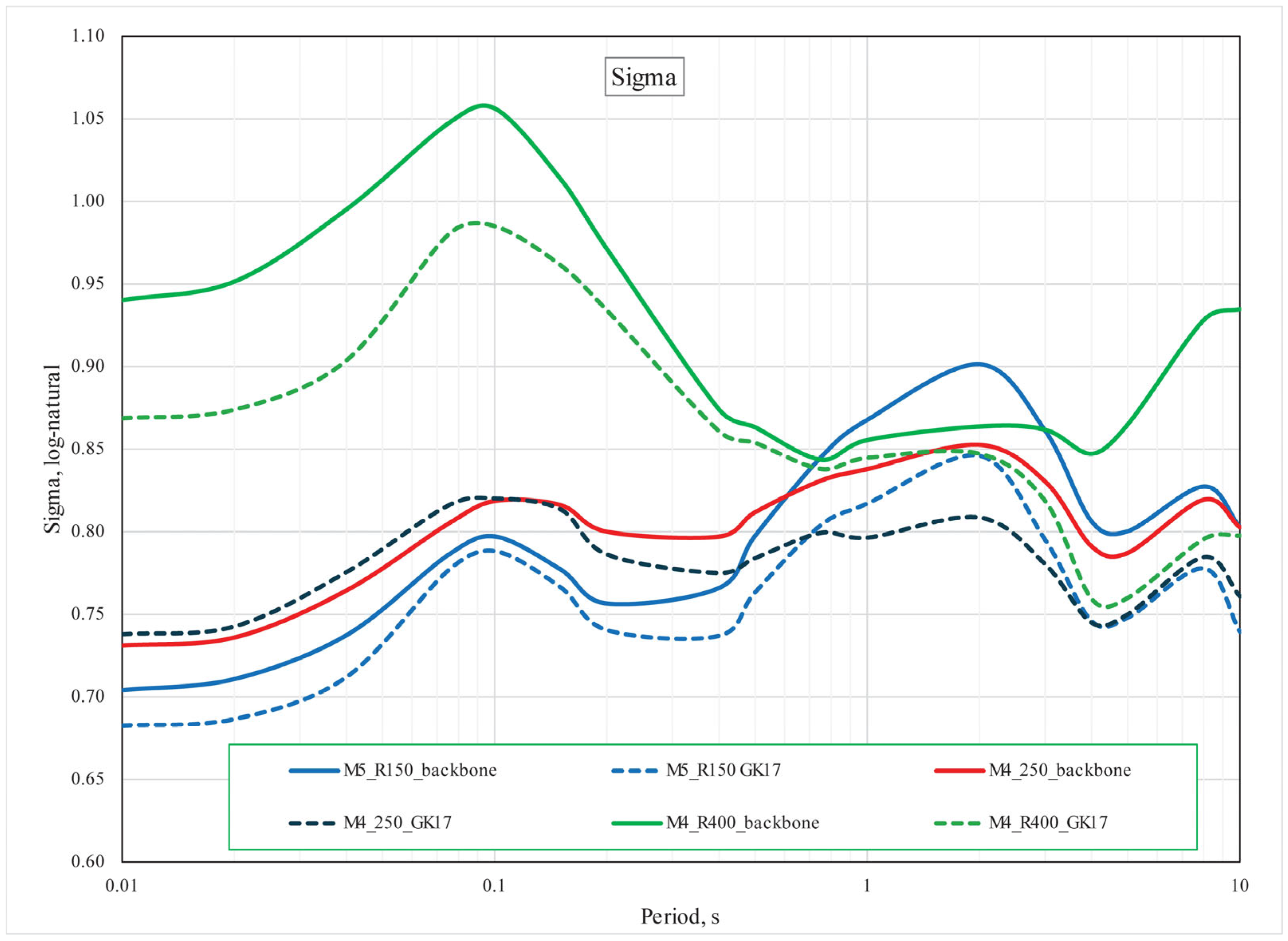
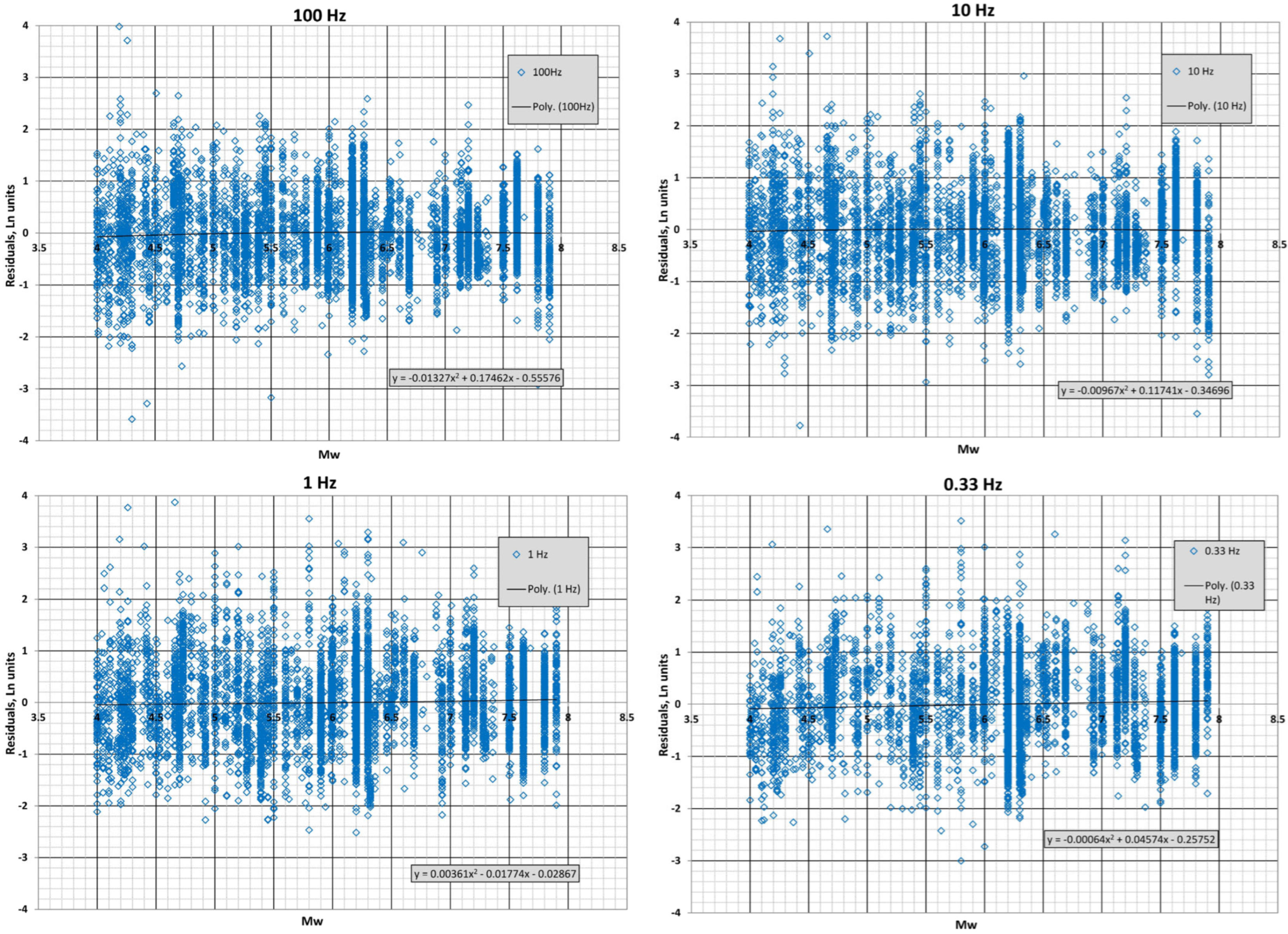
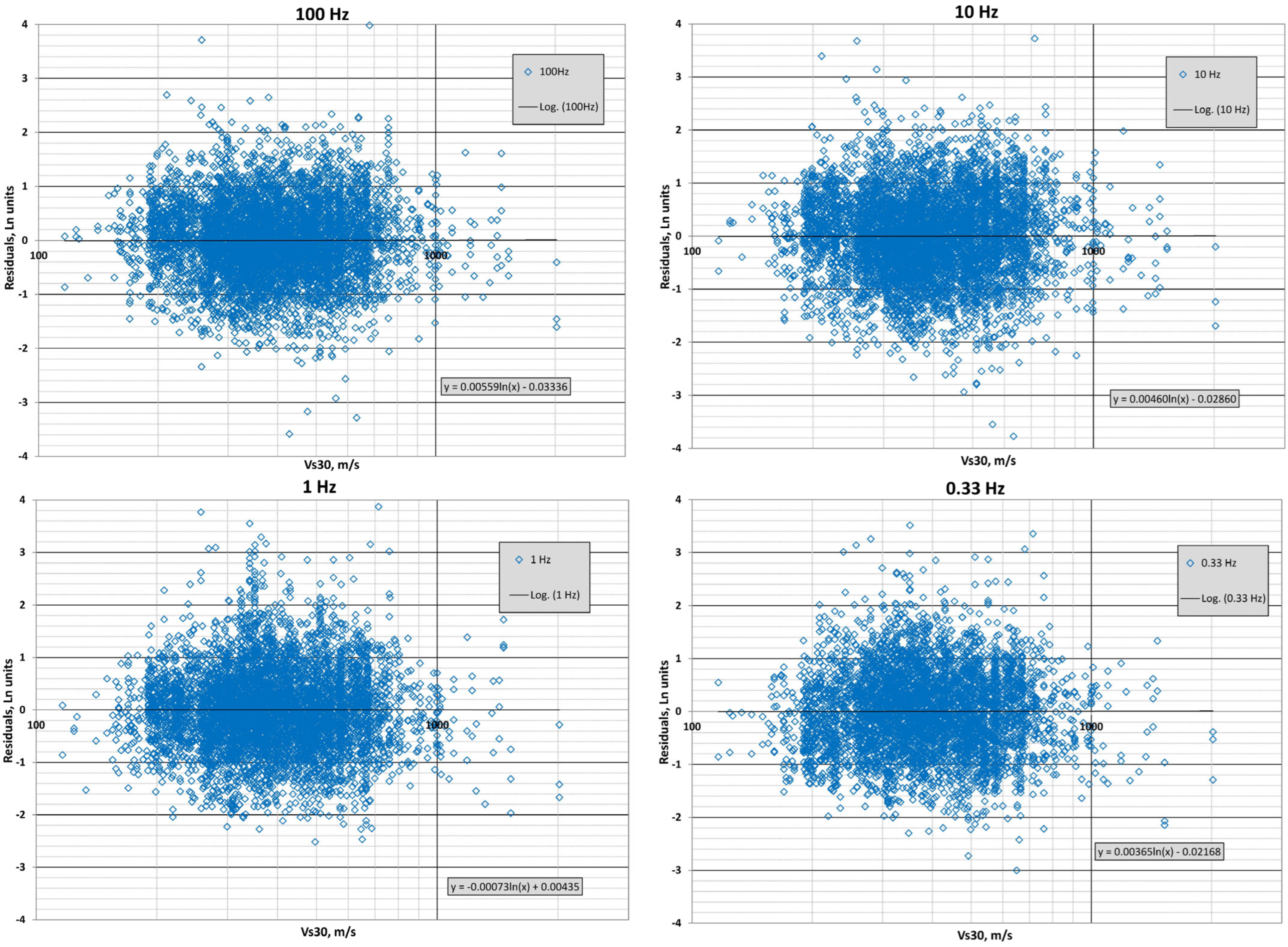
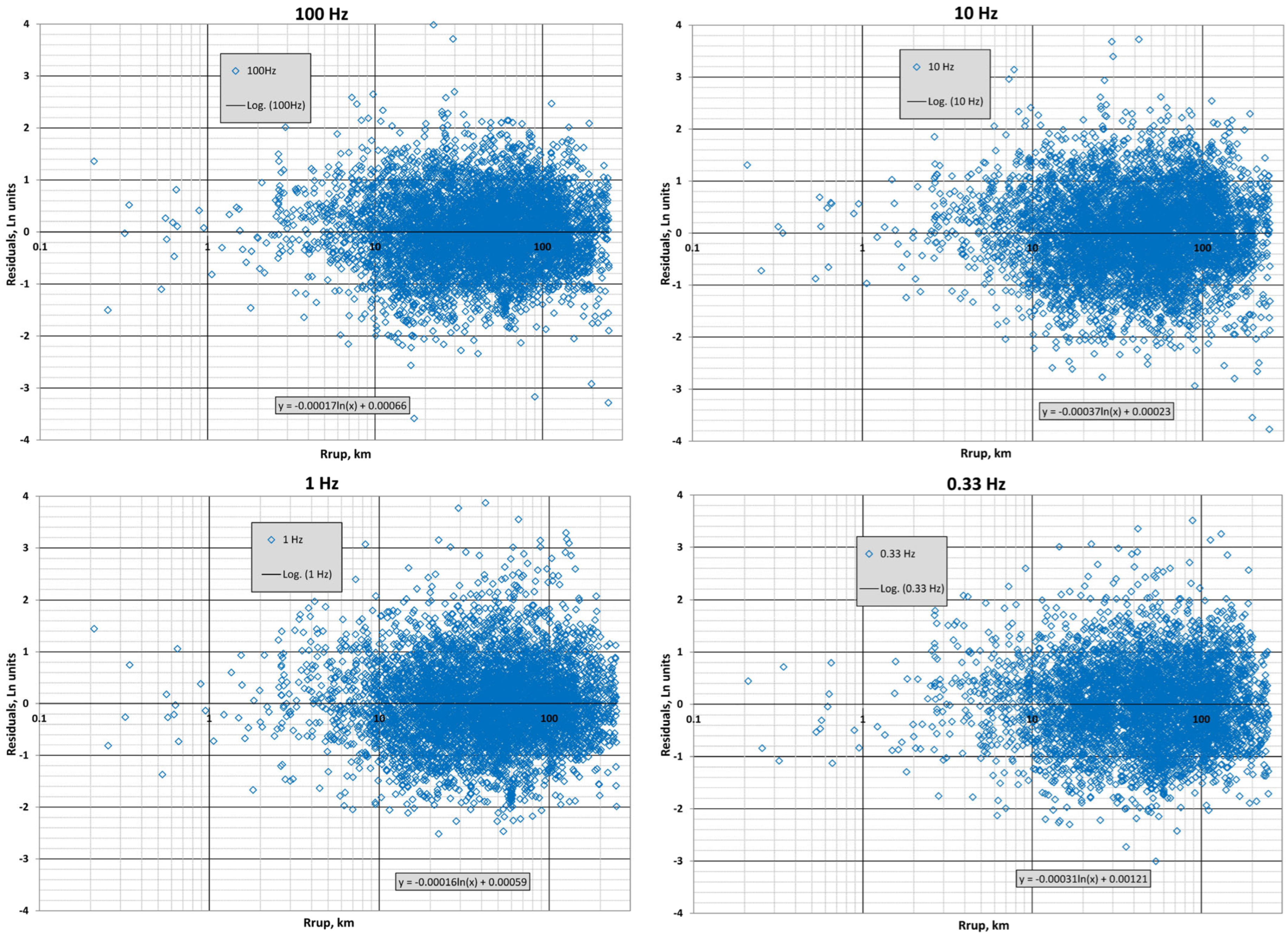
5. Results
6. Data and Resources
Author Contributions
Funding
Data Availability Statement
Acknowledgments
Conflicts of Interest
References
- Joyner, W.B.; Boore, D.M. Methods for regression analysis of strong-motion data. Bull. Seismol. Soc. Am. 1993, 83, 469–487. [Google Scholar] [CrossRef]
- Joyner, W.B.; Boore, D.M. Errata: Methods for regression analysis of strong-motion data. Bull. Seismol. Soc. Am. 1994, 84, 955–956. [Google Scholar] [CrossRef]
- Brillinger, D.R.; Preisler, H.K. An exploratory analysis of the Joyner-Boore attenuation data. Bull. Seismol. Soc. Am. 1984, 74, 1441–1450. [Google Scholar]
- Brillinger, D.R.; Preisler, H.K. Further analysis of the Joyner-Boore attenuation data. Bull. Seismol. Soc. Am. 1985, 75, 611–614. [Google Scholar] [CrossRef]
- Abrahamson, N.A.; Youngs, R.R. A stable algorithm for regression analyses using the random effects model. Bull. Seismol. Soc. Am. 1992, 82, 505–510. [Google Scholar] [CrossRef]
- Abrahamson, N.A.; Silva, W.J.; Kamai, R. Summary of the ASK14 Ground Motion Relation for Active Crustal Regions. Earthq. Spectra 2014, 30, 1025–1055. [Google Scholar] [CrossRef]
- Boore, D.M.; Stewart, J.P.; Seyhan, E.; Atkinson, G.M. NGA-West2 Equations for Predicting PGA, PGV, and 5% Damped PSA for Shallow Crustal Earthquakes. Earthq. Spectra 2014, 30, 1057–1085. [Google Scholar] [CrossRef]
- Campbell, K.W.; Bozorgnia, Y. NGA-West2 Ground Motion Model for the Average Horizontal Components of PGA, PGV, and 5% Damped Linear Acceleration Response Spectra. Earthq. Spectra 2014, 30, 1087–1115. [Google Scholar] [CrossRef]
- Chiou, B.; Youngs, R.R. Update of the Chiou and Youngs NGA Model for the Average Horizontal Component of Peak Ground Motion and Response Spectra. Earthq. Spectra 2014, 30, 1117–1153. [Google Scholar] [CrossRef]
- Campbell, K.W. Prediction of Strong Ground Motion Using the Hybrid Empirical Method and its Use in the Development of Ground-Motion (Attenuation) Relations in Eastern North America. Bull. Seismol. Soc. Am. 2003, 93, 1012–1033. [Google Scholar] [CrossRef]
- Pezeshk, S.; Zandieh, A.; Campbell, K.W.; Tavakoli, B. Ground-motion prediction equations for central and eastern North America using the hybrid empirical method and NGA-West2 empirical ground-motion models. Bull. Seismol. Soc. Am. 2018, 108, 2278–2304. [Google Scholar] [CrossRef]
- Khosravikia, F.; Clayton, P.; Nagy, Z. Artificial neural network-based framework for developing ground-motion models for natural and induced earthquakes in Oklahoma, Kansas, and Texas. Seismol. Res. Lett. 2019, 90, 604–613. [Google Scholar] [CrossRef]
- Fayaz, J.; Xiang, Y.; Zareian, F. Generalized ground motion prediction model using hybrid recurrent neural network. Earthq. Eng. Struct. Dyn. 2021, 50, 1539–1561. [Google Scholar] [CrossRef]
- Klimasewski, A.; Sahakian, V.; Thomas, A. Comparing artificial neural networks with traditional ground-motion models for small-magnitude earthquakes in Southern California. Bull. Seismol. Soc. Am. 2021, 20, 1577–1589. [Google Scholar] [CrossRef]
- Withers, K.B.; Moschetti, M.P.; Thompson, E.M. A Machine Learning Approach to Developing Ground Motion Models from Simulated Ground Motions. Geophys. Res. Lett. 2020, 47, e2019GL086690. [Google Scholar] [CrossRef]
- Alidadi, N.; Pezeshk, S. Ground-Motion Model for Small-to-Moderate Potentially Induced Earthquakes Using an Ensemble Machine Learning Approach for CENA. Bull. Seismol. Soc. Am. 2024, 114, 2202–2215. [Google Scholar] [CrossRef]
- Alidadi, N.; Pezeshk, S. State of the art: Application of machine learning in ground motion modeling. Eng. Appl. Artif. Intell. 2025, 149, 110534. [Google Scholar] [CrossRef]
- Douglas, J. Ground Motion Prediction Equations 1964–2023 (Incomplete); Figshare: London, UK, 2024. [Google Scholar] [CrossRef]
- Paredes Estacio, J.L.; De Risi, R. Historical evolution of the input parameters of ergodic and non-ergodic ground motion models (GMMs): A review. Earth-Sci. Rev. 2025, 266, 105074. [Google Scholar] [CrossRef]
- Graizer, V.; Kalkan, E. Ground-motion attenuation model for peak horizontal acceleration from shallow crustal earthquakes. Earthq. Spectra 2007, 23, 585–613. [Google Scholar] [CrossRef]
- Graizer, V.; Kalkan, E. Prediction of response spectral acceleration ordinates based on PGA attenuation. Earthq. Spectra 2009, 25, 39–69. [Google Scholar] [CrossRef]
- Graizer, V.; Kalkan, E. Modular filter-based approach to ground-motion attenuation modeling. Seismol. Res. Lett. 2011, 82, 21–31. [Google Scholar] [CrossRef]
- Graizer, V. Alternative (G-16v2) Ground Motion Prediction Equations for Central and Eastern North America. Bull. Seismol. Soc. Am. 2017, 107, 869–886. [Google Scholar] [CrossRef]
- Graizer, V. GK17 Ground-Motion Prediction Equation for Horizontal PGA and 5% Damped PSA from Shallow Crustal Continental Earthquakes. Bull. Seismol. Soc. Am. 2018, 108, 380–398. [Google Scholar] [CrossRef]
- Wilson, H.B.; Turcotte, H.L.; Halpern, D. Advanced Mathematics and Mechanics Applications Using MATLAB, 3rd ed.; Chapman & Hall/CRC: Boca Raton, FL, USA, 2003; p. 696. [Google Scholar]
- Graizer, V. Application of GK17 Ground-Motion Model to Preliminary Processed Turkish Ground-Motion Recordings Dataset and GK Model Adjustment to the Turkish Environment by Developing Partially Nonergodic Model. Seismol. Res. Lett. 2024, 95, 651–663. [Google Scholar] [CrossRef]
- Ancheta, T.D.; Darragh, R.B.; Stewart, J.P.; Seyhan, E.; Silva, W.J.; Chiou, B.S.-J.; Wooddell, K.E.; Graves, R.W.; Kottke, A.R.; Boore, D.M.; et al. NGA-West2 database. Earthq. Spectra 2014, 30, 989–1005. [Google Scholar] [CrossRef]
- Buckreis, T.E.; Güryuva, B.; İçen, A.; Okcu, O.; Altindal, A.; Aydin, M.F.; Pretell, R.; Sandikkaya, A.; Kale, O.; Askan, A.; et al. Ground Motion Data from the 2023 Türkiye-Syria Earthquake Sequence. DesignSafe-CI 2023, 1–2+63. [Google Scholar] [CrossRef]
- Buckreis, T.E.; Güryuva, B.; İçen, A.; Okcu, O.; Altindal, A.; Aydin, M.F.; Pretell, R.; Sandikkaya, A.; Kale, O.; Askan, A.; et al. Ground Motions. In Turkey Earthquakes: Report on Geoscience Engineering Impacts; Earthquake Engineering Research Institute: Oakland, CA, USA, 2023; Chapter 3; pp. 63–94. [Google Scholar] [CrossRef]
- Graizer, V.; Stovall, S.; Bauer, L. Global GS24 Ground Motion Models for Active Crustal Regions Based on Non-Traditional Modeling Approach. In Technical Letter Report [TLR-RES-DE-SGSEB-2024-01]; U.S. Nuclear Regulatory Commission: Washington, DC, USA, 2024; ADAMS ML24309A090; p. 45. [Google Scholar]
- Boore, D.M. Orientation-independent, nongeometric-mean measures of seismic intensity from two horizontal components of motion. Bull. Seismol. Soc. Am. 2010, 100, 1830–1835. [Google Scholar] [CrossRef]
- Douglas, J.; Halldorsson, B. On the use of aftershocks when deriving ground-motion prediction equations. In Proceedings of the 9th US National and 10th Canadian Conference on Earthquake Engineering (9USN/10CCEE), Toronto, ON, Canada, 25–29 July 2010; Volume 2010, pp. 7456–7465. [Google Scholar]
- Idriss, I.M. NGA-West2 model for estimating average horizontal values of pseudo-absolute spectral accelerations generated by crustal earthquakes. In Report PEER 20013/08; Pacific Earthquake Engineering Research Center, University of California: Berkeley, CA, USA, 2013. [Google Scholar]
- Graizer, V.; Kalkan, E. Summary of the GK15 Ground-Motion Prediction Equation for Horizontal PGA and 5% Damped PSA from Shallow Crustal Continental Earthquakes. Bull. Seismol. Soc. Am. 2016, 106, 687–707. [Google Scholar] [CrossRef]
- Graizer, V. Ground-Motion Prediction Equations for Central and Eastern North America. Bull. Seismol. Soc. Am. 2016, 106, 1600–1612. [Google Scholar] [CrossRef]
- Graizer, V. Geometric spreading and apparent anelastic attenuation of response spectral accelerations. Soil Dyn. Earthq. Eng. 2022, 162, 107463. [Google Scholar] [CrossRef]
- Idriss, I.M.; Sun, J.I. SHAKE91: A Computer Program for Conducting Equivalent Linear Seismic Response Analyses of Horizontally Layered Soil Deposits; Center for Geotechnical Modeling Department of Civil & Environmental Engineering, University of California: Berkeley, CA, USA, 1992. [Google Scholar]
- Kottke, A.R.; Rathje, E.M. Technical Manual for Strata, Report 2008/10; Pacific Earthquake Engineering Research (PEER) Center: Berkeley, CA, USA, 2008; p. 95. [Google Scholar]
- Gibbs, J.F.; Fumal, T.E.; Boore, D.M.; Joyner, W.B. Seismic velocities and geological logs from borehole measurements at seven strong-motion stations that recorded the Loma Prieta earthquake. In U.S. Geol. Surv. Open-File Rept. 92-287; U.S. Geological Survey: Menlo Park, CA, USA, 1992; p. 139. [Google Scholar]
- De Alba, P.; Nigbor, R.L.; Steidl, J.H.; Stepp, J.C. (Eds.) Proceedings of the International Workshop for Site Selection, Installation, and Operation of Geotechnical Strong-Motion Arrays; COSMOS: Los Angeles, CA, USA, 2004; p. 245. [Google Scholar]
- Kamai, R.; Abrahamson, N.A.; Silva, W.J. Nonlinear horizontal site amplification for constraining the NGA-West2 GMPEs. Earthq. Spectra 2014, 30, 1223–1240. [Google Scholar] [CrossRef]
- Walling, M.; Silva, W.J.; Abrahamson, N.A. Nonlinear site amplification factors for constraining the NGA models. Earthq. Spectra 2008, 24, 243–255. [Google Scholar] [CrossRef]
- Laurendeau, A.; Cotton, F.; Ktenidou, O.-J.; Bonilla, L.-F.; Hollender, F. Rock and stiff-soil site amplification: Dependencies on VS30 and kappa (κ0). Bull. Seismol. Soc. Am. 2013, 103, 3131–3148. [Google Scholar] [CrossRef]
- Ktenidou, O.-J.; Abrahamson, N. Empirical estimation of high-frequency ground motion on hard rock. Seism. Res. Lett. 2016, 87, 1465–1478. [Google Scholar] [CrossRef]
- Kishida, T.; Haddadi, H.; Darragh, R.B.; Kayen, R.E.; Silva, W.J.; Bozorgnia, Y. Apparent Wave Velocity and Site Amplification at the California Strong Motion Instrumentation Program Carquinez Bridge Geotechnical Arrays During the 2014 M6.0 South Napa Earthquake. Earthq. Spectra 2018, 34, 327–347. [Google Scholar] [CrossRef]
- Graizer, V. Effect of low-pass filtering and re-sampling on spectral and peak ground acceleration in strong-motion records. In Proceedings of the 15 World Conference on Earthquake Engineering, Lisbon, Portugal, 24–28 September 2012. [Google Scholar]
- Erickson, D.; McNamara, D.E.; Benz, H.M. Frequency-dependent Lg Q within the continental United States. Bull. Seism. Soc. Am. 2004, 94, 1630–1643. [Google Scholar] [CrossRef]
- Malagnini, L.; Mayeda, K.; Urhammer, R.; Akinci, A.; Herrmann, R.B. A regional ground-motion excitation/attenuation model for the San Francisco region. Bull. Seismol. Soc. Am. 2007, 97, 843–862. [Google Scholar] [CrossRef]
- Mayeda, K.; Malagnini, L.; Phillips, W.S.; Walter, W.R.; Dreger, D. 2-D or not 2-D, that is the question: A northern California test. Geophys. Res. Lett. 2005, 32, L12301. [Google Scholar] [CrossRef]
- Ford, S.R.; Dreger, D.S.; Mayeda, K.; Walter, W.R.; Malagnini, L.; Philips, W.S. Regional attenuation in northern California: A comparison of five 1D Q methods. Bull. Seism. Soc. Am. 2008, 98, 2033–2046. [Google Scholar] [CrossRef]
- Chapman, M.; Conn, A. A model for Lg propagation in the Gulf Coastal Plain of the southern United States. Bull. Seismol. Soc. Am. 2016, 106, 349–363. [Google Scholar] [CrossRef]
- Boatwright, J.; Bundock, H.; Luetgert, J.; Seekins, L.; Gee, L.; Lombard, P. The dependence of PGA and PGV on distance and magnitude inferred from Northern California ShakeMap data. Bull. Seismol. Soc. Am. 2003, 93, 2043–2055. [Google Scholar] [CrossRef]
- Morozov, I.B. Geometrical attenuation, frequency dependence of Q, and the absorption band problem. Geophys. J. Int. 2008, 175, 239–252. [Google Scholar] [CrossRef]
- Booth, E. The Estimation of Peak Ground-motion Parameters from Spectral Ordinates. J. Earthq. Eng. 2007, 11, 13–32. [Google Scholar] [CrossRef]

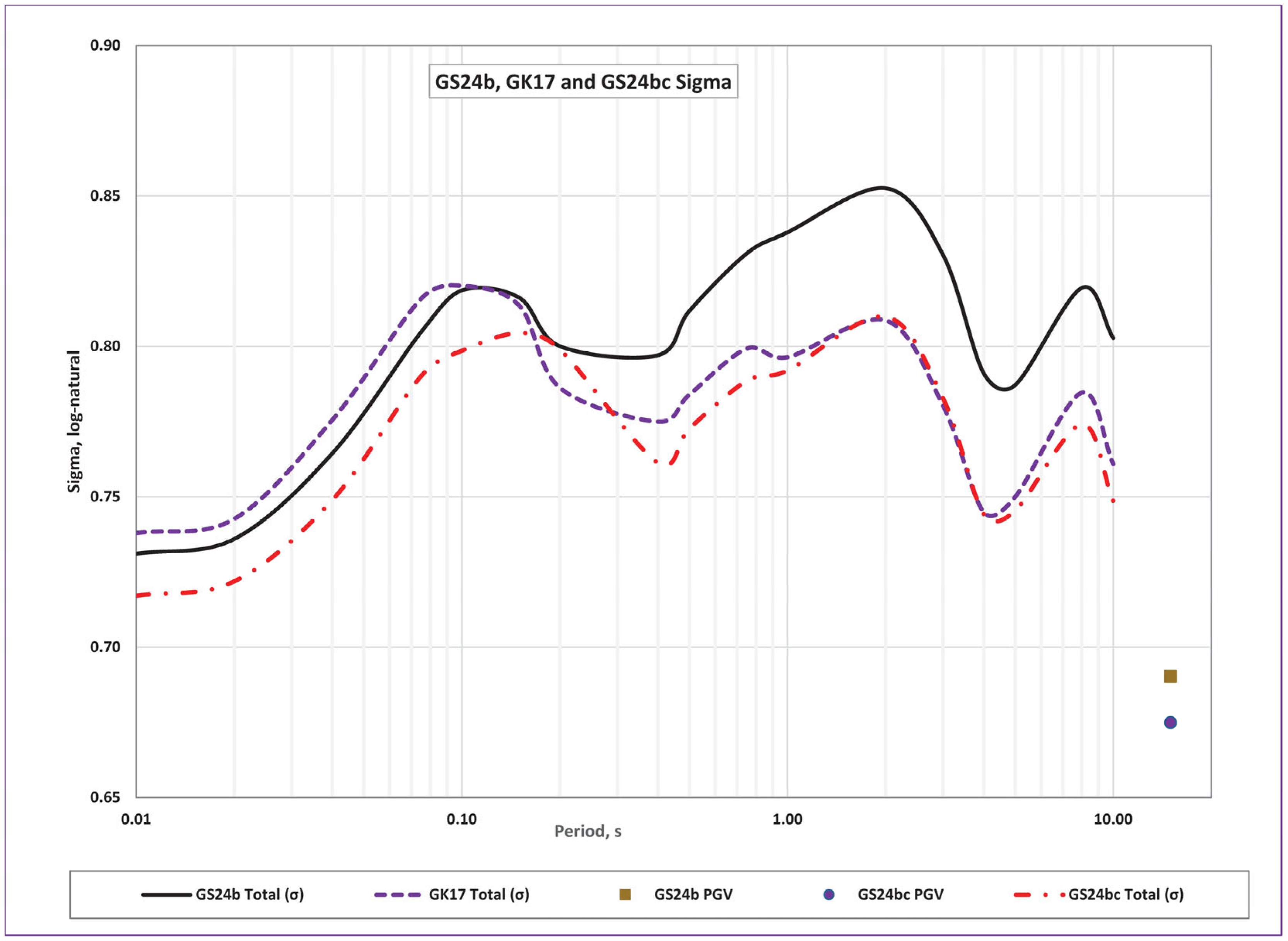
| GS24b Standard Deviations | GK17 Standard Deviations | GS24bc Standard Deviations | |||||||
|---|---|---|---|---|---|---|---|---|---|
| Period, s | GS24b Total (σ) | GS24b Within-Event (ϕ) | GS24b Between-Event (τ) | GK17 Total (σ) | GK17 Within-Event (ϕ) | GK17 Between-Event (τ) | GS24bc Total (σ) | GS24bc Within-Event (ϕ) | GS24bc Between-Event (τ) |
| 0.01 | 0.731 | 0.541 | 0.492 | 0.738 | 0.526 | 0.517 | 0.717 | 0.532 | 0.481 |
| 0.02 | 0.736 | 0.549 | 0.490 | 0.743 | 0.532 | 0.518 | 0.722 | 0.538 | 0.481 |
| 0.04 | 0.764 | 0.565 | 0.515 | 0.776 | 0.547 | 0.550 | 0.749 | 0.552 | 0.506 |
| 0.08 | 0.805 | 0.591 | 0.546 | 0.816 | 0.580 | 0.573 | 0.790 | 0.586 | 0.530 |
| 0.10 | 0.819 | 0.599 | 0.558 | 0.820 | 0.589 | 0.570 | 0.799 | 0.597 | 0.530 |
| 0.15 | 0.816 | 0.597 | 0.556 | 0.814 | 0.590 | 0.560 | 0.804 | 0.599 | 0.538 |
| 0.20 | 0.800 | 0.582 | 0.548 | 0.786 | 0.576 | 0.535 | 0.799 | 0.583 | 0.546 |
| 0.40 | 0.797 | 0.587 | 0.539 | 0.775 | 0.574 | 0.521 | 0.761 | 0.585 | 0.487 |
| 0.50 | 0.812 | 0.597 | 0.550 | 0.784 | 0.581 | 0.526 | 0.773 | 0.593 | 0.495 |
| 0.75 | 0.831 | 0.610 | 0.564 | 0.799 | 0.590 | 0.540 | 0.789 | 0.605 | 0.506 |
| 1.00 | 0.838 | 0.607 | 0.578 | 0.796 | 0.582 | 0.544 | 0.792 | 0.600 | 0.517 |
| 2.00 | 0.853 | 0.626 | 0.579 | 0.809 | 0.599 | 0.543 | 0.810 | 0.614 | 0.528 |
| 3.00 | 0.830 | 0.608 | 0.566 | 0.780 | 0.585 | 0.516 | 0.783 | 0.600 | 0.502 |
| 4.00 | 0.791 | 0.581 | 0.537 | 0.745 | 0.561 | 0.490 | 0.744 | 0.575 | 0.473 |
| 5.00 | 0.787 | 0.562 | 0.552 | 0.750 | 0.545 | 0.516 | 0.745 | 0.553 | 0.500 |
| 8.00 | 0.819 | 0.578 | 0.581 | 0.785 | 0.558 | 0.552 | 0.774 | 0.553 | 0.542 |
| 10.00 | 0.803 | 0.581 | 0.553 | 0.761 | 0.558 | 0.517 | 0.749 | 0.544 | 0.515 |
| PGV | 0.684 | 0.501 | 0.466 | 0.677 | 0.480 | 0.478 | 0.675 | 0.482 | 0.473 |
Disclaimer/Publisher’s Note: The statements, opinions and data contained in all publications are solely those of the individual author(s) and contributor(s) and not of MDPI and/or the editor(s). MDPI and/or the editor(s) disclaim responsibility for any injury to people or property resulting from any ideas, methods, instructions or products referred to in the content. |
© 2025 by the authors. Licensee MDPI, Basel, Switzerland. This article is an open access article distributed under the terms and conditions of the Creative Commons Attribution (CC BY) license (https://creativecommons.org/licenses/by/4.0/).
Share and Cite
Graizer, V.; Stovall, S. GS24b and GS24bc Ground Motion Models for Active Crustal Regions Based on a Non-Traditional Modeling Approach. Geosciences 2025, 15, 277. https://doi.org/10.3390/geosciences15080277
Graizer V, Stovall S. GS24b and GS24bc Ground Motion Models for Active Crustal Regions Based on a Non-Traditional Modeling Approach. Geosciences. 2025; 15(8):277. https://doi.org/10.3390/geosciences15080277
Chicago/Turabian StyleGraizer, Vladimir, and Scott Stovall. 2025. "GS24b and GS24bc Ground Motion Models for Active Crustal Regions Based on a Non-Traditional Modeling Approach" Geosciences 15, no. 8: 277. https://doi.org/10.3390/geosciences15080277
APA StyleGraizer, V., & Stovall, S. (2025). GS24b and GS24bc Ground Motion Models for Active Crustal Regions Based on a Non-Traditional Modeling Approach. Geosciences, 15(8), 277. https://doi.org/10.3390/geosciences15080277