Optimizing Geophysical Inversion: Versatile Regularization and Prior Integration Strategies for Electrical and Seismic Tomographic Data

Abstract

The increasing demand for high-resolution subsurface imaging has driven significant advances in geophysical inversion methodologies. Despite the availability of various software packages for electrical resistivity tomography (ERT), time-domain induced polarization (TDIP), and seismic refraction tomography (SRT), significant challenges remain in selecting optimal regularization parameters and in the effective incorporation of prior information into the inversion process. In this study, we propose new strategies to address these critical issues by developing versatile and flexible tools for electrical and seismic tomographic data inversion. Specifically, we introduce two automated procedures for regularization parameter selection: a full loop method (fixed-λ optimization) where the regularization parameter is kept constant during the inversion process, and a single-inversion approach (automaticLam) where it varies throughout the iterations. Additionally, we present a novel constrained inversion strategy that effectively balances prior information, minimizes data misfit, and promotes model smoothness. This approach is thoroughly compared with the state-of-the-art methods, demonstrating its superiority in maintaining model reliability and reducing dependence on subjective operator choices. Applications to synthetic, laboratory, and real-world case studies validate the efficacy of our strategies, showcasing their potential to enhance the robustness of geophysical models and standardize the inversion process, ensuring its independence from operator decisions.

1. Introduction

Over the past few years, interest in tomographic reconstruction of the subsurface using geophysical data has grown considerably, driven by the increasing demand for high-resolution models. This need is critical for effective near-surface imaging in civil and environmental engineering (e.g., [1,2]). Among the available geophysical methods, electrical resistivity tomography (ERT) and seismic refraction tomography (SRT) are widely used due to their flexibility, cost-effectiveness, and ability to link geophysical measurements with petrophysical parameters (e.g., [3]). Additionally, the induced polarization (IP) method—which investigates the capacitive response of the subsurface—is frequently employed in scenarios where a pronounced IP effect is expected, such as in clay-rich environments or anthropogenic settings like landfills and contaminated sites (e.g., [4]).

Over the past three decades, numerous software packages have been developed for electrical (ERT and IP) and seismic (SRT) data inversion. As an example, ERT/IP data inversion can be performed using closed-source software such as RES2DINV/RES3DINV (Geotomo software), AarhusInv [5], or ERTLab (Geostudi Astier and Multiphase Technologies) or, working with open-source packages such as ResIPy [6] or IP4DI [7]. Similarly, closed-source packages such as Rayfract (Intelligent Resources Inc.) or ReflexW (Sandmeier geophysical research) can be employed for SRT data inversion as well as open-source codes like the recent RefraPy [8] or PyRefra [9], the latter mainly focused on seismic data treatment. However, few codes are capable of handling both ERT and IP and SRT data, among which SimPEG [10] and PyGIMLi [11] are undoubtedly the most applied in recent years. Although almost every code is characterized by its forward solver both for ERT/IP and SRT, they share a local inversion approach for data inversion, based on a Tikhonov-regularized least squares algorithm [12,13].

Despite the large number of available software packages, however, certain issues remain unaddressed, leaving room for further development of flexible and comprehensive codes. More specifically, because the inverse problem is inherently data-driven, it is essential to maintain a flexible approach that can tailor the inversion process to the specific dataset under examination.

One of the most critical challenges in inversion is still the automation of residual subjective decisions, such as the choice of regularization parameters and the proper handling and incorporation of prior information, which is often available in engineering projects (i.e., borehole data or direct geophysical measurements). Among the various approaches for the automatic selection of regularization parameters aimed at reducing subjectivity (e.g., [14]), the L-curve criterion is one of the most widely used. However, its effectiveness is limited when the curve deviates from the ideal shape (e.g., [15]), which can make the criterion unreliable in practice.

To this end, we developed flexible and versatile algorithms for the processing, modeling, and inversion of ERT, SRT, and time-domain induced polarization (TDIP), applicable to both laboratory and field settings, including datasets defined on meshes that account for topography. Specifically, our main contributions are (i) a twofold algorithm for the automatic selection of the regularization parameter, consisting of a full loop procedure (fixed-λ optimization) where the parameter is kept constant during the inversion, and a single-inversion procedure (automaticLam) for cases where the parameter varies across iterations. The latter was developed by adapting the approach originally proposed by Zhdanov et al. [16]; (ii) a tool that allows the inversion process to be tailored to specific case studies by incorporating prior information, either through inequality constraints, by constraining the solution to a reference model or through a novel constrained inversion strategy based on prior data.

After the description of the theoretical principles underlying our algorithms Section 2, applications to synthetic (SYN) SRT data, laboratory (LAB) ERT, and real-world (RW) landfill ERT/TDIP examples are discussed in Section 3.

2. The Inversion Algorithm

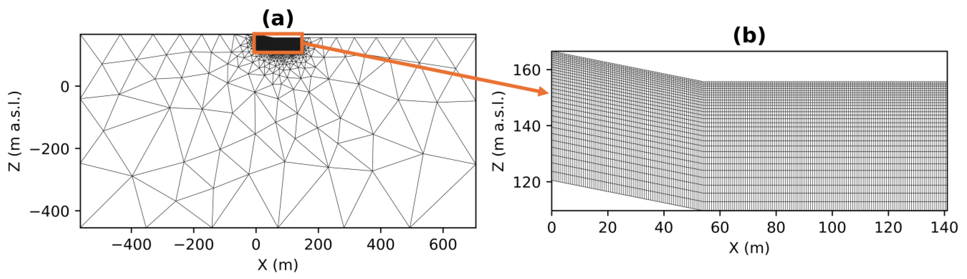
We implemented a procedure for the whole processing phase of tomographic data, from meshing to modeling and inversion, with automation of many steps as well as allowing for multiple choices of regularization parameters and insertion of prior information.

2.1. Meshing

The meshes used for the inversion of SRT and ERT/TDIP data have different requirements. While the forward modeling and inversion of seismic data can be performed on a single mesh whose extent is determined by the acquisition layout, electrical measurements require a two-step meshing procedure to properly handle both modeling and inversion. Specifically, solving the geoelectrical forward problem requires extending the domain boundaries well beyond the source positions to correctly apply boundary conditions [17]. Additionally, further mesh refinement in regions with high potential gradients is essential to minimize errors [18]. Conversely, similarly to SRT data processing, the inversion can be performed on a coarser parameter mesh, with the horizontal dimension determined by the length of the electrode array. To this end, we developed the meshing module FlexiMesh, which can generate structured meshes able to handle both the seismic and the two-step electrical procedures. The forward electrical mesh is derived from the parameter grid by adding an external region, made up of triangular elements with progressively larger dimensions to reduce the computational time (Figure 1a), and it is further refined in the parametric zone by bisecting cell edges to better handle the high potential gradients in such a region. FlexiMesh incorporates electrode and shot/geophone points as fixed nodes of the mesh and allows the user to select the number of additional nodes placed on the surface around each sensor. Additionally, it can accommodate complex topographies through interpolation of sensor coordinates (reader can refer to [19] for cases involving more complex topography). The height of the cells is set equal to their width by default, but it can be customized by changing the vertical vs. horizontal ratio or logarithmically increasing it with depth to compensate for the typical loss of resolution of geoelectrical methods (Figure 1b).

2.2. Forward Modeling

In both electrical and seismic methods, accurate forward modeling of geophysical observations is essential for ensuring a robust inversion process and to obtain reliable subsurface models. In our algorithms, ERT and SRT forward calculations rely on the open-source pyGIMLi package [11], which enables the calculation of apparent resistivities based on the secondary potential technique [18]. In this approach, the total potential u is split up into a primary and a secondary part, u = u_p + u_s, where u_p is analytically computed though the continuity equation for a given background conductivity σ_p, usually a homogeneous half-space, and u_s accounts for the perturbation caused by conductivity heterogeneities. The secondary potential u_s satisfies the following partial differential equation:

$$\nabla ·\left(\sigma \nabla u_s\right)=-\nabla ·\left[\right(\sigma -{\sigma }_p)\nabla u_p]$$

(1)

where σ denotes the actual (spatially variable) conductivity distribution. This formulation improves numerical stability and accuracy near electrodes and conductivity discontinuities [18]. Observed traveltimes are computed through Dijkstra’s algorithm [20], according to which the traveltime at node j is computed by [21]:

$$t_j=\underset{i\in \mathcal{N}\left(j\right)}{\mathit{min}}(t_i+l_{ij}{s}_{ij})$$

(2)

where t_i is the known traveltime at node i, l_ij is the distance between nodes i and j, s_ij is the slowness (reciprocal of velocity) along that segment, and $𝒩$(j) denotes the set of neighboring nodes directly connected to node j, i.e., the set of predecessors of node j in the graph. Dijkstra’s algorithm [20] arranges the order of nodes to be updated so that after several iterations the shortest paths are found.

On the other hand, the TDIP forward solution is calculated through the nonlinear perturbation model introduced by Oldenburg and Li [22], which considers the IP model as a small perturbation of the base resistivity model [23]. According to Seigel [24], in fact, the effect of the intrinsic chargeability M is to decrease the instantaneous conductivity σ_∞ to the direct current (DC) value σ₀:

$${\sigma }_0=(1-M){\sigma }_{\infty }$$

(3)

The TDIP response can be thus obtained through

$$M_a={\displaystyle \frac{f\left({\sigma }_0\right)-f\left({\sigma }_{\infty }\right)}{f\left({\sigma }_0\right)}}$$

(4)

in which f is the forward operator acting on a resistivity model (i.e., the reciprocal of conductivity). According to Equation (4), apparent chargeability can be computed by carrying out two resistivity forward calculations considering instantaneous and DC resistivity models, with the former originating from Seigel’s definition.

2.3. Inversion

Whatever the considered tomographic dataset, our inversion framework is always the same, with a different data transformation applied for each case. Let m be the model parameters vector, whose dimension is equal to the number of cells of the inversion mesh, and d the data vector, containing the transformed observed values. On the one hand, m always holds log-transformed model parameters; on the other hand, the values in d are determined based on the investigation type: ERT observations are log-transformed, while TDIP and SRT measurements are always handled without any conversion. Each data point is associated with an error ε_i (i.e., the relative stacking error in the case of ERT and TDIP data), which can be considered within the inversion procedure through the data weighting matrix D, containing on its main diagonal the reciprocals of data errors. In the case of SRT data, a uniform error is assumed for all values, set to 3% by default, and the same approach can be applied to ERT and TDIP measurements if stacking errors are affected by low reliability, as may occur when a low number of stacks is performed. Given the high ill-posedness of the inverse problem associated with minimizing the weighted residual between data and forward response f(m), Tikhonov and Arsenin [13] proposed adding a stabilizing term, commonly a smoothness constraint term to better constrain the under-determined inverse problem and improve the model’s characteristics [12]. This term is incorporated into the functional to be minimized through a weighting factor λ, resulting in the final objective function written using an l₂-norm,

$$\Phi ={\Phi }_d+\lambda {\Phi }_m={‖\mathbf{D}(\mathbf{d}-f(\mathbf{m}\left)\right)‖}_2^2+{\lambda ‖\mathbf{C}\mathbf{m}‖}_2^2,$$

(5)

in which matrix C is a first-order or second-order operator with the option to set a weight for vertical anisotropy in the sense of Constable et al. [12]. The objective function is nonlinear, since both electrical and seismic forward problems are nonlinear, and so to minimize it we used a first-order Taylor expansion (i.e., the Gauss–Newton method) obtaining the least squares problem:

$$\left({\widehat{\mathbf{S}}}^T{\mathbf{D}}^T\mathbf{D}\widehat{\mathbf{S}}+\lambda {\mathbf{C}}^T\mathbf{C}\right)\mathsf{\Delta }{\mathbf{m}}^{p+1}={\widehat{\mathbf{S}}}^T{\mathbf{D}}^T\mathbf{D}(\mathbf{d}-f({\mathbf{m}}^p\left)\right)-\lambda {\mathbf{C}}^T\mathbf{C}{\mathbf{m}}^p$$

(6)

with p being the iteration number and $\widehat{\mathbf{S}}$ the scaled Jacobian or sensitivity matrix, derived from its linear form S to account for logarithmic transformation according to the chain rule (dividing it for the derivatives of the model transformation and multiplying it for the derivatives of data transformation). S contains the partial derivatives of model responses with respect to the model parameters:

$$S_{ m,n}^p={\displaystyle \frac{{\partial \left(f\left({\mathbf{m}}^p\right)\right)}_m}{\partial {\left(m\right)}_n}}$$

(7)

where the subscripts m and n indicate the row and column of the matrix element being calculated. Several methods exist to obtain sensitivities or Fréchet derivatives (e.g., [25]). In our algorithm, electrical sensitivities are computed following the formulation of Kemna [26], which was developed from Sasaki [17], while seismic sensitivities are computed using ray-based derivatives with optional Fresnel volume weighting, combining classical ray theory [27] and fat-ray approaches [28].

Equation (6) can be interpreted as the least squares solution of the following system formulated in terms of model perturbation:

$$\left[\begin{array}{c}\mathbf{D}\widehat{\mathbf{S}}\\ \sqrt{\lambda }\mathbf{C}\end{array}\right]\left[\mathsf{\Delta }{\mathbf{m}}^{p+1}\right]=\left[\begin{array}{c}\mathbf{D}(\mathbf{d}-f({\mathbf{m}}^p)\\ -\sqrt{\lambda }\mathbf{C}{\mathbf{m}}^p\end{array}\right].$$

(8)

Our algorithms can solve the regularized normal equations in Equation (6) with an exact solver, or the system in Equation (8) in a least squares sense by using the LSQR algorithm [29]. Although there is no significant difference between the two approaches and the resulting models are fully comparable, the system in Equation (8) proves useful for the straightforward incorporation of additional terms, as will be discussed later when dealing with the topic of including prior information. In both cases, the solution of the system is followed by an additional line search step at each iteration to prevent the model from overshooting because of nonlinearity. During this procedure, a range of τ parameters between 0 and 1 is tested to identify the value that minimizes the total functional (Equation (5)), updating the model for the next iteration according to

$${\mathbf{m}}^{p+1}={\mathbf{m}}^p+\tau \mathsf{\Delta }{\mathbf{m}}^{p+1}.$$

(9)

To avoid increasing computational costs, the forward responses required for each line search calculation are based on a linearization of the responses corresponding to τ = 0 (the response from the previous iteration) and τ = 1, requiring only one additional forward computation per iteration:

$$f\left(\tau \right)=f\left(0\right)+\tau (f\left(1\right)-f\left(0\right)).$$

(10)

Although more computationally expensive formulations may yield a more precise fit of the exact forward calculation, linear interpolation proves adequate for estimating the line search parameter without significantly increasing computational costs while promoting improved convergence [30].

The inversion process ends when no additional reduction in data misfit is obtained from one iteration to the next. For this purpose, the stopping criterion is based on the relative root mean squared error (RRMSE) for the inversion of resistivity and traveltime data, and on the mean absolute error (MAE) for the inversion of chargeability datasets, defined as

$$RRMSE \left(\%\right)=\sqrt{{\displaystyle \frac{1}{n}}{\sum }_{i=1}^n{\left({\displaystyle \frac{d_i^{obs}-d_i^{calc}}{d_i^{obs}}}\right)}^2}\times 100,$$

(11a)

$$MAE={\displaystyle \frac{1}{n}}{\sum }_{i=1}^n\left|d_i^{obs}-d_i^{calc}\right|,$$

(11b)

where d_i^obs is the generic observed data, d_i^calc the corresponding prediction, and n the total number of the observations. This choice is driven by the lower magnitude of TDIP measurements, which is more suitable for absolute rather than relative error evaluation [31]. In any case, the inversion concludes when the error measure’s relative reduction is lower than a fixed threshold (1%) compared to the previous iteration.

2.3.1. Blocky Inversion

Equation (6) (or, similarly, the least squares solution of Equation (8)) enforces the minimization of the squared spatial variations (“roughness”) of the inverted quantities, resulting in smooth transitions between adjacent cells. However, in specific scenarios, minimizing an l₁-norm may be preferable to an l₂-norm. This approach is particularly advantageous when outliers are present in the data [32], as it employs a robust norm that mitigates their influence during inversion. Additionally, it is beneficial when the subsurface geology comprises largely homogeneous regions separated by sharp boundaries [33].

We implemented this approach, commonly referred to as “blocky inversion”, by adapting the standard least squares formulation through the Iteratively Reweighted Least Squares (IRLS) algorithm [34]. The system in Equation (6) becomes

$$\left({\widehat{\mathbf{S}}}^T{\mathbf{D}}^T{\mathbf{R}}_d\mathbf{D}\widehat{\mathbf{S}}+\lambda {\mathbf{C}}^T{\mathbf{R}}_m\mathbf{C}\right)\mathsf{\Delta }{\mathbf{m}}^{p+1}={\widehat{\mathbf{S}}}^T{\mathbf{D}}^T{\mathbf{R}}_{\mathit{d}}\mathbf{D}(\mathbf{d}-f({\mathbf{m}}^p\left)\right)-\lambda {\mathbf{C}}^T{\mathbf{R}}_{\mathit{m}}\mathbf{C}{\mathbf{m}}^p$$

(12)

where R_d and R_m are two diagonal weighting matrices whose elements are set to balance the weight of different elements of data and model misfits following the approach proposed by Wolke and Schwetlick [35]. R_d is built at the beginning of the inversion process based on the observed data, while R_m is iteratively updated using the values of the current model parameters. In this case, since the minimization of the l₁-norm of the total functional is performed, it is more appropriate to express the relative error using a linear rather than a quadratic estimation. For this reason, the misfit associated with the blocky inversion of ERT and SRT data is quantified in terms of the Mean Absolute Percentage Error (MAPE):

$$MAPE \left(\%\right)={\displaystyle \frac{1}{n}}{\sum }_{i=1}^n\left|{\displaystyle \frac{d_i^{obs}-d_i^{calc}}{d_i^{obs}}}\right|\times 100.$$

(13)

2.3.2. Selection of the Regularization Parameter

The regularization weighting parameter λ balances data fitting and model smoothness, requiring appropriate selection. Lower values result in rough models with strong data adherence, whereas higher values yield smoother models with weaker data fitting [13]. Two main categories of approaches can be identified for managing this parameter during the inversion process: fixed-λ methods, where the value set in the first iteration remains constant throughout the inversion, and variable-λ methods, where the parameter is updated at each iteration based on a predefined criterion. Many approaches have been proposed for the automatic selection of this parameter (e.g., [14]), but, in the current state-of-the-art, no recognized optimal strategy exists. A particularly popular approach is the L-curve method, in which λ is determined at each iteration by balancing the trade-off between data fit and model roughness. This is achieved by plotting Φ_d against Φ_m for a wide range of λ values and identifying the point of maximum curvature as the optimal solution. The method derives its name from the typical L-shaped appearance of the curve; however, in some cases, the curve may deviate from this shape, making this criterion inadequate [15].

Another issue with this approach is that it is reliable only for well-linearizable problems, as it does not include the line search step [30]. For these reasons, Günther [30] suggested selecting the regularization parameter using the fixed-λ approach, starting with a first-guess λ and changing it according to the inversion error until the optimal compromise is found. Although this approach is quite intuitive, it heavily depends on the operator’s decisions.

We introduced two different methods for λ selection, for both fixed- and variable-λ strategies. The first approach, called fixed-λ optimization, is based on performing n complete inversions, each with a different fixed-λ parameter from a wide set (the geometric progression of 19 values between 1 and 10⁵ by default). Such a range should be sufficiently broad and abundant to ensure a reliable choice, but, at the same time, not excessively large so as to avoid an extreme increase in computational costs. At the end of this automated process, the curve of the achieved data fitting is computed (measured in the same way as the convergence criterion) as a function of λ. Figure 2 shows the results of such analysis applied to the RW case study. In general, this curve can exhibit two distinct trends: it may present an internal minimum, as shown in Figure 2a for ERT inversion of the RW case, or it may display a monotonically increasing trend, as shown in Figure 2b for TDIP inversion at the same site. In the first case, it is intuitive to assume the optimal value corresponds to the minimum. In the latter case, the R² plot is computed starting from the first two points and progressively adding one point, identifying the optimal values as the ones for which this value drops below a predefined threshold (0.90), achieving the best compromise between data fitting and model roughness according to an objective and repeatable criterion. Following this procedure, the optimal fixed-λ values found for the RW field case are 100 for resistivity (Figure 2a) and 316 for chargeability (Figure 2b,c).

Zhdanov et al. [16] introduced a novel variable-λ approach, which has been proven effective in a few studies for the inversion of magnetotelluric data [36,37] and for gravity data [38]. In this approach, the first iteration is a pure minimization of data misfit, setting λ⁰ = 0. Then, the first regularization value introduces a strong regularization:

$${\lambda }^1={\displaystyle \frac{{\Phi }_d^0}{{\Phi }_m^0}}={\displaystyle \frac{{‖\mathbf{D}(\mathbf{d}-f({\mathbf{m}}^0\left)\right)‖}_2^2}{{‖\mathbf{C}{\mathbf{m}}^0‖}_2^2}}.$$

(14)

This selection provides a balance between data misfit and roughness [37]. The values of the following iterations are set according to

$${\lambda }^k={\lambda }^1{\left(q\right)}^{k-1} , k=1, 2, \dots , n$$

(15)

in which k is the iteration number and q is an empirical parameter between 0 and 1 that defines the rate of decrease of the regularization parameter. Zhdanov et al. [37] suggested selecting this parameter by running several inversions with different q values and evaluating the final error and the stability of the inverted models. We adopt such a strategy for variable-λ inversions, calling this method automaticLam, and apply it for the first time to electrical and seismic tomographic data. Even though a specific criterion to find the q parameter can be defined, we found that it consistently yielded similar values for the same geophysical methods, and therefore fixed it to 0.5 for ERT and TDIP data (analogous to the findings of Rezaie et al. [38]) and to 0.8 for SRT data. In this way, such a method requires performing a single inversion process in which each iteration involves a single forward calculation, resulting in a significantly reduced computational cost. Additionally, since λ⁰ can sometimes lead to a model m⁰ presenting some negative values, an internal control is implemented, setting the λ⁰ value to the smallest possible value greater than zero, if such a circumstance occurs. Moreover, although such a situation has never occurred in our applications, it may be advisable to set a minimum λ (very low) to prevent it from approaching zero in the final iterations. In Section 3, the automaticLam and fixed-λ optimization methods will be compared with reference to the RW case.

2.3.3. Prior Information

Incorporating prior information into the inversion process is a recurring challenge in inverse problems, and numerous strategies have been proposed to address it. Such information can vary in nature (e.g., geological or geophysical) and may relate to specific areas of the inverted model (local constraints) or to the whole section (global constraints). A widely used approach involves applying inequality constraints [39]:

$$\mathbf{m}=\ln {\displaystyle \frac{\mathbf{p}-\mathbf{a}}{\mathbf{b}-\mathbf{p}}}$$

(16)

in which p is the unchanged parameters vector and a and b are two vectors containing the lower and upper bounds for the transformation of each model’s element. This approach is typically employed to ensure physically consistent values setting wide bounds for each vector (global constraints, e.g., avoiding negative values), but, if more knowledge is available regarding some parts of the model, it can be used to restrict local values within a known range. By default, we apply inequality constraints to define logarithmic global model transformation, as discussed in Section 2.3. A different classical approach involves the use of a reference model m₀ [12], incorporated into Equation (5) as follows:

$${\Phi }_m={‖\mathbf{C}(\mathbf{m}-{\mathbf{m}}_0)‖}_2^2.$$

(17)

The m₀ model can be either global or local. For the latter case, rows of m₀ corresponding to areas without prior knowledge are set to zero, and only the smoothness constraint acts in the corresponding cells. However, this approach implies that the weighting term λ is the same for both smoothness and prior incorporation, which can be misleading in many cases.

To address this issue, we introduce a novel constrained inversion with prior data approach, adding a specific third term to the standard cost function:

$$\Phi ={‖\mathbf{D}(\mathbf{d}-f(\mathbf{m}\left)\right)‖}_2^2+\lambda {‖\mathbf{C}\mathbf{m}‖}_2^2+\gamma {‖{\mathbf{C}}_{prior}(\mathbf{p}-{\mathbf{p}}_0)‖}_2^2,$$

(18)

where γ is a weighting constant that controls the strength of the prior constraint, C_prior is a diagonal matrix with ones in the rows corresponding to the cells where prior information is available and zeros elsewhere, and p₀ is a vector containing the prior information (not filled where prior knowledge is not available). Minimizing the relation in Equation (18) leads to the following system to be solved in a least squares sense:

$$\left[\begin{array}{c}\mathbf{D}\widehat{\mathbf{S}}\\ \sqrt{\lambda }\mathbf{C}\\ \sqrt{\gamma }{\widehat{\mathbf{C}}}_{prior}\end{array}\right]\left[\Delta {\mathit{m}}^{p+1}\right]=\left[\begin{array}{c}\mathbf{D}(\mathbf{d}-f({\mathbf{m}}^p)\\ -\sqrt{\lambda }\mathbf{C}{\mathbf{m}}^p\\ \sqrt{\gamma }\left({\mathbf{p}}_0-{\widehat{\mathbf{C}}}_{prior}{\mathbf{m}}^p\right)\end{array}\right],$$

(19)

where ${\widehat{\mathbf{C}}}_{prior}$ is a scaled matrix built by multiplying C_prior for the reciprocals of the partial derivatives of m with respect to p because of logarithmic transformation according to the chain rule. For selecting the γ parameter, we define the γ-optimization approach, for which γ is changed over a wide range and the resulting inversion errors are analyzed. Figure 3 illustrates such optimization applied to the LAB dataset: for small γ values, the inversion is equivalent to a classical inversion without prior constraint, achieving the same error (horizontal red dotted line). As γ increases (starting from γ = 10⁻³), the error decreases due to a model closer to prior knowledge. The optimal γ is then identified by the minimum error (vertical green dashed line in Figure 3). As γ becomes excessively large, the error increases, and the inversion process is dominated by the prior constraint (in this specific case it becomes constant as the model transitions to a homogeneous medium based on the a priori value).

It can be easily observed that the inequality constraints allow for the definition of a variation range for model parameters, whereas both the reference model and the constrained inversion with prior data approaches introduce an equality constraint, whose strength is controlled by a regularization term. Nevertheless, inequality constraints can also be applied in the presence of exact prior knowledge by setting the bounds very close to the constraint. This, however, results in a rigid model transformation due to the absence of a specific weighting. In Section 3.2, such aspects will be further analyzed with reference to the LAB case.

3. Examples

The versatile inversion procedure described above is applied to three examples (SYN, LAB, and RW as defined in the Introduction) corresponding to synthetic, laboratory, and field data. The selection of these examples was driven by the need to demonstrate the capability of the proposed inversion strategies across a wide range of datasets and applications.

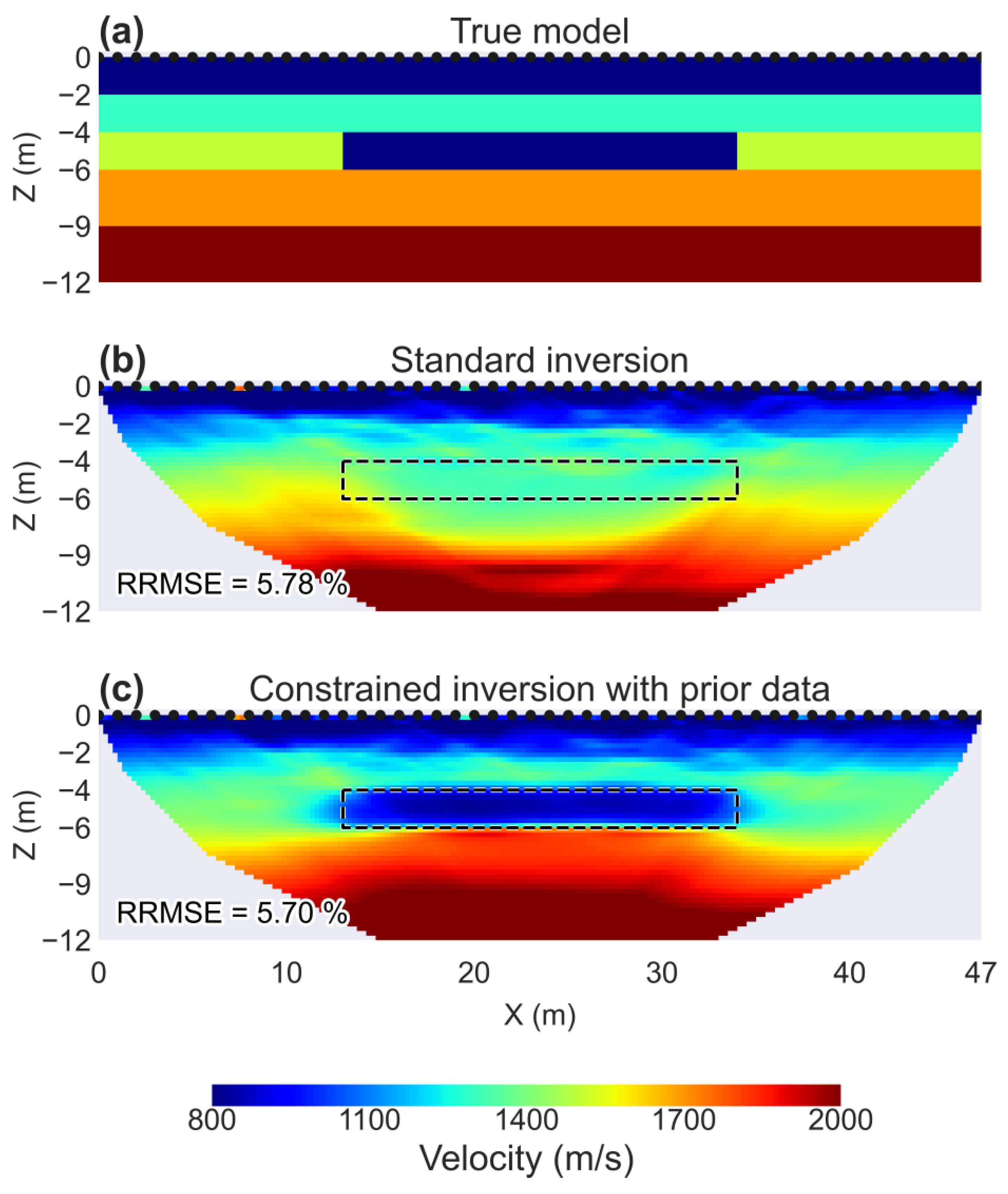
3.1. SYN: SRT Data in the Case of Velocity Inversion

Firstly, a synthetic velocity model was developed by modifying the one proposed by Yari et al. [40], with the aim of testing our software on a challenging example incorporating a velocity inversion, which is a case often encountered in the near-surface region. In fact, velocity inversions are frequent in many geological scenarios, such as alluvial plains, where stiff sediments (e.g., gravel or sand) can overlie softer ones (e.g., silt or soft clays), volcanic successions (e.g., tuff overlying pozzolanic ash), or an anthropogenic environment (e.g., concrete above soil). Therefore, we built a five-layer model with thicknesses of 2 m for the first three layers and 3 m for the deeper ones for a maximum depth of investigation of 12 m (Figure 4a). P-wave velocity values gradually increase from a minimum of 800 m/s (shallow layer) to a maximum of 2000 m/s (deep layer), simulating a depositional sequence transitioning from fine- to coarse-grained sediments. Within the intermediate layer (v_P = 1500 m/s), a low-velocity zone was included in the middle of the model (x = 13–34 m) to simulate the velocity inversion due to a lens of fine-grained deposits. The SRT survey was reproduced by 48 sensors spaced 1 m apart and 1 shot every 2 sensors. Then, the synthetic dataset was contaminated by a zero-mean Gaussian error with a standard deviation of 0.3 ms. The results are shown in Figure 4b,c for the standard inversion and the inversion incorporating prior data, respectively. This method simulates the case where a borehole is drilled in the neighborhood of the SRT line and P-wave velocity values are available from, e.g., a downhole investigation, which is not infrequent in many near-surface oriented projects (e.g., [41]). It is clear that, despite an overall good reconstruction of the main layers using standard inversion (Figure 4b), the velocity inversion (highlighted by a black dashed rectangle) cannot be detected without incorporating prior information into the inversion scheme. Conversely, the low-velocity inclusion is well detected both for the shape and the depth interval by the constrained inversion with prior data (Figure 4c). The benefit of the latter approach also extends to the reconstruction of the deep layers (v_P = 1700 m/s and 2000 m/s), while only minor differences are observed between the two inversion approaches for the shallow low-velocity layers. This outcome is expected due to the improved ray coverage in the shallow region. Both procedures converge to a similar final misfit (RRMSE = 5.70% and 5.08%, respectively), indicating the non-uniqueness of the solution. This non-uniqueness can affect accuracy, particularly near the bottom and in the lateral zones (where ray coverage is limited), as well as in the case of velocity inversions (which may be bypassed by the rays).

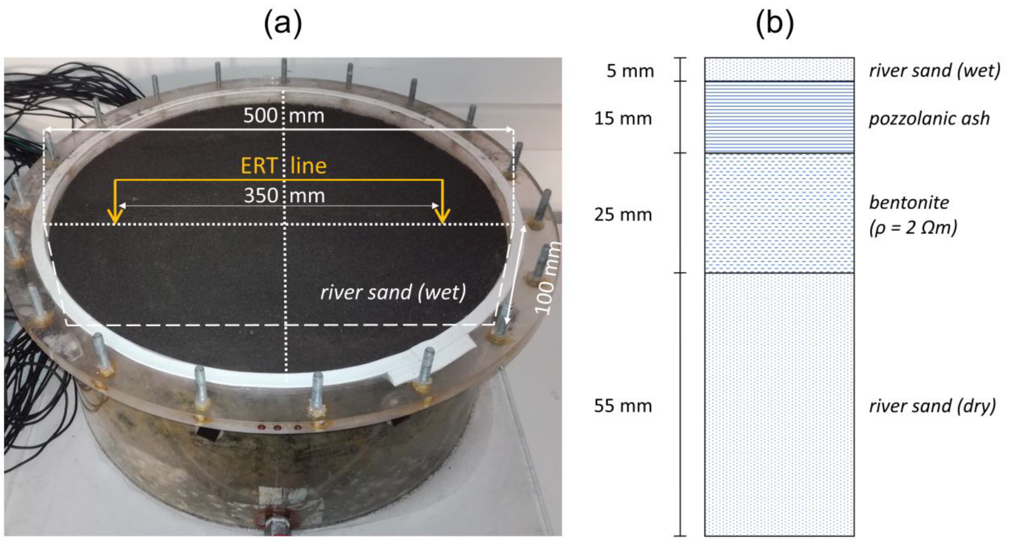
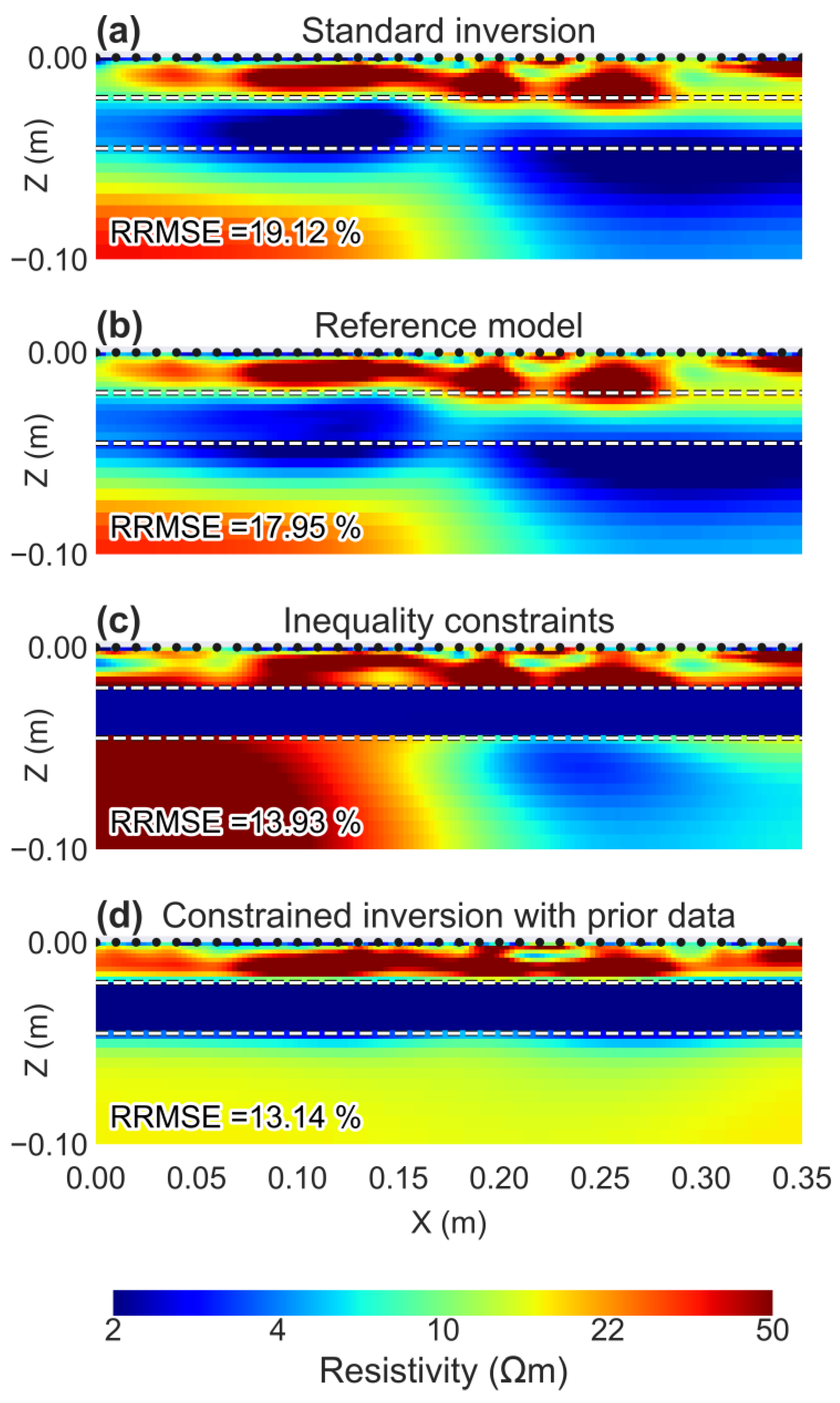
3.2. LAB: ERT Data for a Laboratory Model

A laboratory model was constructed in a Plexiglas tank with a height of 20 cm and a diameter of 50 cm (Figure 5a, see [42] for full details of the holder). The tank was filled with a multi-layer configuration, from top to bottom (Figure 5b): (i) a 5 mm thick river sand layer and (ii) a 15 mm thick pozzolanic ash layer, both sieved at 0.1 mm and (partially) saturated from the top; (iii) a 25 mm thick bentonite (clay) layer and (iv) a dry sand bottom layer (55 mm thick). Gravel was also added at the bottom of the sample (depth between 10 and 20 cm), separated from the overlying layers by a nonwoven fabric. This model was chosen because it is representative of a typical near-surface sequence of a shallow aquifer/aquiclude, often encountered in alluvial plains. The pozzolanic ash and river sand layers were progressively added in compacted increments of 10 mm. The bentonite layer was prepared by mixing bentonite powder Bentosund 120E with tap water at a 1:1 weight ratio. The resistivity of the bentonite clay, measured using a 1D device (with a horizontal field applied), was 2.0 ± 0.1 Ωm.

The ERT line is made of 48 gold electrodes mounted on a Plexiglas string and spaced 10 mm apart, having a diameter of 2 mm and a length of 20 mm, with 2 mm embedded within the sample. The grounded length of the electrodes was enough to ensure a good contact resistance (between 1 and 5 kΩ), without affecting the point-source hypothesis [43].

We selected for the measurements only the 36 electrodes located in the middle portion of the sample to avoid boundary effects due to the closeness of the external Plexiglas surface acting as an insulator. The ERT dataset was acquired with an IRIS SyscalPro48 resistivity meter, connected via two switch boxes to the electrodes and using a multiple gradient array for a total number of 378 apparent resistivity measurements. Filtering of raw data led to the removal of many outliers concentrated on the right side of the section, which was more affected by noise due to a faulty electrode (the last one) and a local reduction in water content in the ultra-shallow portion of the sample. The decreased water content reduced the current in this zone, resulting in a lower signal-to-noise ratio.

Since these challenging experimental conditions are frequent for field investigations, where contact resistances can vary significantly along the ERT line, we left the sample unchanged without providing additional watering on the right side.

We performed four different inversions of the apparent resistivity dataset. both without and with the inclusion of prior information. In the latter case, prior knowledge was inserted during inversion by means of the three approaches described in Section 2.3.3. Specifically, inequality constraints in the range [1.9–2.1 Ωm] were applied to the layer between 20 and 45 cm (clay), where the prior information is available from the direct measurements of resistivity. The inverted models are shown in Figure 6, which highlights the benefit of the application of the constrained inversion procedure with respect to the other approaches. The standard inversion (Figure 6a) can depict the three-layer model in the left part of the sample, while suffering from low resolution and accuracy in the right part, due to the poor data coverage. The two shallow layers display strong variability, likely due to the different water content, being more conductive in the left part than in the right part in the ultra-shallow sand layer (linked to the variable lower current levels), and higher resistivity in the underlying pozzolanic ash (∼20–50 Ωm). The transition between the pozzolanic ash and clay layers is quite well reconstructed, while the deep clay–sand interface shows lower accuracy, particularly in the right portion of the sample. Constraining inversion to a reference model (Figure 6b) slightly improves the final misfit (≈18%), even if the model remains largely unchanged.

Forcing the solution in the intermediate layer through inequality constraints (Figure 6c) can significantly reduce the misfit (≈14%) but at the cost of affecting the consistency of the model in the deep layer (sand), which shows a sharp, unrealistic vertical transition between a resistive (left) and a conductive (right) zone. Finally, the model resulting from the constrained inversion with prior data (Figure 6d) further reduces the misfit (≈13%) and is well in agreement with the true layering. In this case, the choice of γ (regularization of prior data) was made by the γ-optimization procedure described in Section 2.3.3, where γ is changed in the range [10⁻¹⁰–10³⁰], finding the optimum value (γ_opt = 10²²) corresponding with the minimum RRMSE. The relatively low resistivity values reconstructed for the deep dry sand layer (∼10 Ωm) can be ascribed to the low sensitivity associated to these pixels, which is often responsible for a biased estimation of the resistivity values of bedrock or basal geological layers.

3.3. RW: ERT/TDIP for Landfill Detection

The last presented case study, taken from [4], concerns the field investigation of uncontrolled waste disposal located in Central Italy, where ERT and TDIP methods were applied to detect the presence of the waste mass and to assess its depth and lateral extension. Among the three lines surveyed at the site, we selected the L2 profile, as it was conducted partly inside and partly outside the landfill, facilitating the identification of unauthorized waste disposal. The ERT/TDIP line consisted of 48 electrodes spaced 3 m apart and connected to the IRIS SyscalPro48, with a dipole–dipole array (a_max = 5 and n_max = 6). IP data were collected with a pulse duration of 1 s (50% duty cycle) and a delay time of 20 ms, and the decay curve was sampled logarithmically using 20 gates.

Firstly, we evaluated the optimal regularization parameter using the fixed-λ optimization procedure for both resistivity and chargeability data, finding the values in the error-λ space, as shown in Figure 2. Secondly, the automaticLam criterion was applied, and the results of the two methods were compared. All inversion routines were run on a computer equipped with 4 cores/8 threads, an Intel Xeon E3-1270 v3 CPU at 3.50 GHz and 16 GB RAM. Figure 7 shows the comparison in terms of regularization parameters (Figure 7a,b for resistivity and chargeability, respectively), error progress with iterations (Figure 7c,d), and computational effort (Figure 7e,f). The final errors provided by the two methods are similar for chargeability inversion, while for resistivity there are significant differences both in terms of RRMSE (4.11% for automaticLam vs. 5.07% for fixed-λ optimization) and in the number of iterations needed to achieve convergence (8 instead of 17). On the one hand, using automaticLam we can speed up the choice of the regularization parameters about 20 times for resistivity and 30 times for chargeability in this specific case compared to the full optimization (Figure 7e,f). On the other hand, since the two routines lead to final models that are very similar (Figure 7a–c and Figure 7b–d for resistivity and chargeability, respectively), the automaticLam is confirmed to be the preferable option in a benefit/cost perspective due to its rapidity.

Finally, to investigate the results of the automaticLam routine with a different type of inversion, the inversion algorithm was also run minimizing an l1-norm (blocky inversion). The achieved models (Figure 8e,f) show sharper transitions between the different layers, as expected with the blocky inversion, leading to a generally more reliable reconstruction due to the reduced influence of the smoothness constraint.

4. Discussion

Although many inversion tools are available within the scientific community, the choice of the regularization parameter is often subjective and may introduce biases that undermine the reliability of the resulting models. The two methods proposed in this study are applicable to both fixed-λ and variable-λ strategies. The first approach involves a full loop procedure composed of multiple inversions over a broad range of regularization parameters. While this entails higher computational cost, it consistently returns a single, operator-independent λ-parameter and is flexible to error curves of various shapes, unlike the L-curve criterion, which is effective only when the curve exhibits a specific geometry that is not consistently observed in practice (e.g., [15]). The automaticLam method, on the other hand, is adapted from the framework proposed by Zhdanov et al. [16] for magnetotelluric inversion. This approach has proven effective for both magnetotelluric data (e.g., [36,37]) and gravity data (e.g., [38]). The present study represents its first application to electrical and seismic tomography datasets, demonstrating both significant computational efficiency and improved model reliability. However, since automaticLam employs different values at each iteration, it may be unsuitable for scenarios involving additional terms in the objective function, as in the case of joint inversions (e.g., [19]), where a third term is introduced to link different geophysical properties, or in the approach presented in this paper for incorporating prior information. In such cases, a varying regularization weight across iterations may lead to an imbalance among the different components of the objective function, potentially biasing the final models and compromising a proper trade-off between its terms. Therefore, a fixed-λ optimization routine is preferable in these contexts, as it ensures a constant regularization weight throughout the iterations, thereby providing a more stable basis for identifying suitable weighting for additional terms as well.

This work focuses on a Gauss–Newton inversion scheme with Tikhonov regularization, following the formulation by Tikhonov and Arsenin [13]. In the presence of noisy data, such inversion methods often suffer from non-uniqueness, where different parameterizations can produce similarly fitting models. To address this issue, the proposed tools aim to objectively identify a single optimal regularization parameter, guiding the inversion toward a unique and stable solution. Although models obtained with nearby regularization parameter values may appear similar, assigning a single parameter per dataset simplifies the inversion workflow and mitigates equivalence-related ambiguities commonly encountered in local inversion frameworks [44].

A possible alternative is the Bayesian inversion framework, which seeks to build a posterior distribution over model parameters, offering uncertainty quantification well suited to addressing the inherent non-uniqueness of inverse problems, including ambiguity related to the choice of regularization. However, this comes at the cost of significantly higher computational demand. In this context, the regularization parameters identified through our local criteria may serve as suitable initial estimates for global inversion strategies, such as those employing funnel functions [45], thereby bridging local and probabilistic approaches.

As far as the management of prior information is concerned, a comprehensive comparative assessment of the advantages and limitations of different strategies for incorporating it into the inversion process is still lacking. Our results demonstrate that the novel constrained inversion with prior data approach yields superior results compared to the other two state-of-the-art methods (reference model and inequality constraints), providing more reliable and geologically consistent models. In fact, the classical reference model approach enforces a single weighting factor for both regularization and the integration of prior information, resulting in suboptimal performance due to the inherently different roles and requirements of these two components. Inequality constraints allow for the strict enforcement of prior information without the need for additional parameter tuning or increased computational cost. However, this method does not account for a proper trade-off between prior information, data misfit, and regularization, which can lead to unreliable reconstructions, as observed in the laboratory case.

The constrained inversion with prior data emerges as the only approach among those investigated that is capable of effectively balancing all terms in the objective function. In particular, it allows for an optimal compromise between data misfit minimization, model smoothness, and adherence to prior information, ultimately leading to more reconstructions with reduced error. Despite these advantages, this method still requires greater computational effort compared to the other two, due to the optimization of the additional weighting parameter γ. However, this step is guided by an objective optimization criterion, thus avoiding the subjective bias that could undermine the results if γ were manually selected.

Overall, the effectiveness of prior information incorporation depends strongly on its availability and reliability, which can be challenging in complex or poorly characterized scenarios. In the presented example, the resistivity of a specific layer was directly measured on a physical sample, yielding a highly reliable value due to its very low standard deviation. As shown in Figure 6, such high-quality information can significantly enhance the entire inversion process.

However, when prior information is affected by measurement uncertainty or site-specific variability, its incorporation may mislead the inversion algorithm toward local minima of the misfit function, preventing convergence to the global optimum. Moreover, the acquisition of high-quality prior data can be expensive, as in the case of borehole investigations, thus making geophysical processing without constraints a more practical and cost-effective alternative in many real-world scenarios.

5. Conclusions

We presented a set of versatile procedures for optimizing the inversion of ERT, TDIP, and SRT data. Regarding the selection of the regularization parameter, we described two distinct automatic procedures: one designed for cases in which the parameter remains fixed throughout the inversion (fixed-λ optimization), and the other for cases where it is updated iteratively (automaticLam). The application of these methodologies to the real-world landfill case study enabled a direct comparison of their respective advantages. Specifically, automaticLam provides faster convergence, requiring fewer iterations and reducing computational costs by executing a single inversion instead of a full loop procedure. Conversely, the fixed-λ optimization approach offers an objective and operator-independent selection of λ, which is particularly valuable when the objective function is modified to include additional terms, as it ensures a consistent weighting throughout the inversion process and avoids imbalance among components.

Concerning the incorporation of prior information, the application to the laboratory ERT dataset enabled a clear assessment of the three implemented strategies. Results highlighted the benefits of the proposed method, when compared to two widely adopted and recognized state-of-the-art approaches: the reference model approach and inequality constraints. Although the introduction of a γ-optimization criterion increases the overall computational cost, it ensures an objective trade-off and avoids subjective bias in parameter selection.

Finally, the application to the SRT synthetic case demonstrates that this approach can effectively address common engineering challenges, such as the presence of velocity inversion zones in seismic sections, providing a valuable tool for managing such complex scenarios. More broadly, the method proves effective in all cases where the availability of prior information can significantly improve the reliability of geophysical models.

References

1. Perrone, A.; Lapenna, V.; Piscitelli, S. Electrical resistivity tomography technique for landslide investigation: A review. Earth-Sci. Rev. 2014, 135, 65–82. [Google Scholar] [CrossRef]
2. Soupios, P.; Ntarlagiannis, D. Characterization and Monitoring of Solid Waste Disposal Sites Using Geophysical Methods: Current Applications and Novel Trends; Sengupta, D., Agrahari, S., Eds.; Modelling Trends in Solid and Hazardous Waste Management; Springer: Singapore, 2017. [Google Scholar] [CrossRef]
3. Slater, L. Near Surface Electrical Characterization of Hydraulic Conductivity: From Petrophysical Properties to Aquifer Geometries—A Review. Surv. Geophys. 2007, 28, 169–197. [Google Scholar] [CrossRef]
4. De Donno, G.; Cardarelli, E. Tomographic inversion of time-domain resistivity and chargeability data for the investigation of landfills using a priori information. Waste Manag. 2017, 59, 302–315. [Google Scholar] [CrossRef] [PubMed]
5. Auken, E.; Christiansen, A.V.; Fiandaca, G.; Schamper, C.; Behroozmand, A.A.; Binley, A.; Nielsen, E.; Effersø, F.; Christensen, N.B.; Sørensen, K.I.; et al. An overview of a highly versatile forward and stable inverse algorithm for airborne, ground-based and borehole electromagnetic and electric data. Explor. Geophys. 2015, 46, 223–235. [Google Scholar] [CrossRef]
6. Blanchy, G.; Saneiyan, S.; Boyd, J.; McLachlan, P.; Binley, A. ResIPy, an intuitive open source software for complex geoelectrical inversion/modelling. Comput. Geosci. 2020, 137, 104423. [Google Scholar] [CrossRef]
7. Karaoulis, M.; Revil, A.; Tsourlos, P.; Werkema, D.D.; Minsley, B.J. IP4DI: A software for time-lapse 2D/3D DC-resistivity and induced polarization tomography. Comput. Geosci. 2013, 54, 164–170. [Google Scholar] [CrossRef]
8. Guedes, V.J.C.B.; Maciel, S.T.R.; Rocha, M.P. Refrapy: A Python program for seismic refraction data analysis. Comput. Geosci. 2022, 159, 105020. [Google Scholar] [CrossRef]
9. Zeyen, H.; Léger, E. PyRefra—Refraction seismic data treatment and inversion. Comput. Geosci. 2024, 185, 105556. [Google Scholar] [CrossRef]
10. Cockett, R.; Kang, S.; Heagy, L.J.; Pidlisecky, A.; Oldenburg, D.W. SimPEG: An open source framework for simulation and gradient based parameter estimation in geophysical applications. Comput. Geosci. 2015, 85, 142–154. [Google Scholar] [CrossRef]
11. Rücker, C.; Günther, T.; Wagner, F.M. pyGIMLi: An open-source library for modelling and inversion in geophysics. Comput. Geosci. 2017, 109, 106–123. [Google Scholar] [CrossRef]
12. Constable, S.; Parker, R.L.; Constable, C.G. Occam’s inversion; a practical algorithm for generating smooth models from electromagnetic sounding data. GEOPHYSICS 1987, 52, 289–300. [Google Scholar] [CrossRef]
13. Tikhonov, A.N.; Arsenin, V.Y. Solution of Ill-Posed Problems; Winston and Sons: Washington, DC, USA, 1977. [Google Scholar]
14. Farquharson, C.G.; Oldenburg, D.W. A comparison of automatic techniques for estimating the regularization parameter in non-linear inverse problems. Geophys. J. Int. 2004, 156, 411–425. [Google Scholar] [CrossRef]
15. Vogel, C.R. Non-convergence of the L-curve regularization parameter selection method. Inverse Probl. 1996, 12, 535–547. [Google Scholar] [CrossRef]
16. Zhdanov, M.S. Geophysical Inverse Theory and Regularization Problems; Elsevier: Amsterdam, The Netherlands, 2002. [Google Scholar]
17. Sasaki, Y. Two-dimensional joint inversion of magnetotelluric and dipole-dipole resistivity data. GEOPHYSICS 1989, 54, 254–262. [Google Scholar] [CrossRef]
18. Rücker, C.; Günther, T.; Spitzer, K. Three-dimensional modeling and inversion of dc resistivity data incorporating topography—I. Modelling. Geophys. J. Int. 2006, 166, 495–505. [Google Scholar] [CrossRef]
19. Penta de Peppo, G.; Cercato, M.; De Donno, G. Cross-gradient joint inversion and clustering of ERT and SRT data on structured meshes incorporating topography. Geophys. J. Int. 2024, 239, 1155–1169. [Google Scholar] [CrossRef]
20. Dijkstra, E.W. A note on two problems in connexion with graphs. Numer. Math. 1959, 1, 269–271. [Google Scholar] [CrossRef]
21. Moser, T.J. Shortest path calculation of seismic rays. GEOPHYSICS 1991, 56, 59–67. [Google Scholar] [CrossRef]
22. Oldenburg, D.W.; Li, Y.G. Inversion of induced polarization data. GEOPHYSICS 1994, 59, 1327–1341. [Google Scholar] [CrossRef]
23. Loke, M.H. Tutorial: 2-D and 3-D Electrical Imaging Surveys; Geotomo Software: Houston, TX, USA, 2001. [Google Scholar]
24. Seigel, H.O. Mathematical formulation and type curves for induced polarization. GEOPHYSICS 1959, 24, 547–565. [Google Scholar] [CrossRef]
25. McGillivray, P.R.; Oldenburg, D.W. Methods for calculating frechet derivatives and sensitivities for the non-linear inverse problem: A comparative study. Geophys. Prospect. 1990, 38, 499–524. [Google Scholar] [CrossRef]
26. Kemna, A. Tomographic Inversion of Complex Resistivity. Ph.D. Thesis, Ruhr-Universität, Bochum Institut für Geophysik, 2000. [Google Scholar]
27. Aki, K.; Richards, P.G. Quantitative Seismology, 2nd ed.; University Science Books: Mill Valley, CA, USA, 2002. [Google Scholar]
28. Watanabe, T.; Matsuoka, T.; Ashida, Y. Seismic traveltime tomography using Fresnel volume approach. SEG Tech. Program Expand. Abstr. 1999, 18, 1402–1405. [Google Scholar] [CrossRef]
29. Paige, C.C.; Saunders, M.A. LSQR: An algorithm for sparse linear equations and sparse least squares. ACM Trans. Math. Softw. 1982, 8, 43–71. [Google Scholar] [CrossRef]
30. Günther, T. Inversion Methods and Resolution Analysis for the 2D/3D Reconstruction of Resistivity Structures from DC Measurements. Ph.D. Thesis, Technische Universität Bergakademie Freiberg, Freiberg, Germany, 2004. [Google Scholar] [CrossRef]
31. Sanders, N.R. Measuring forecast accuracy: Some practical suggestions. Prod. Inventory Manag. J. 1997, 38, 43. [Google Scholar]
32. Farquharson, C.G.; Oldenburg, D.W. Non-linear inversion using general measures of data misfit and model structure. Geophys. J. Int. 1998, 134, 213–227. [Google Scholar] [CrossRef]
33. Loke, M.H.; Acworth, I.; Dahlin, T. A comparison of smooth and blocky inversion methods in 2D electrical imaging surveys. Explor. Geophys. 2003, 34, 182–187. [Google Scholar] [CrossRef]
34. Holland, P.W.; Welsch, R.E. Robust regression using iteratively reweighted least-squares. Commun. Stat. —Theory Methods 1977, 6, 813–827. [Google Scholar] [CrossRef]
35. Wolke, R.; Schwetlick, H. Iteratively Reweighted Least Squares: Algorithms, Convergence Analysis, and Numerical Comparisons. SIAM J. Sci. Stat. Comput. 1988, 9, 907–921. [Google Scholar] [CrossRef]
36. Ghaedrahmati, R.; Moradzadeh, A.; Moradpouri, F. An effective estimate for selecting the regularization parameter in the 3D inversion of magnetotelluric data. Acta Geophys. 2022, 70, 609–621. [Google Scholar] [CrossRef]
37. Zhdanov, M.S.; Wan, L.; Gribenko, A.; Čuma, M.; Key, K.; Constable, S. Large-scale 3D inversion of marine magnetotelluric data: Case study from the Gemini prospect, Gulf of Mexico. GEOPHYSICS 2011, 76, F77–F87. [Google Scholar] [CrossRef]
38. Rezaie, M.; Moradzadeh, A.; Kalate, A.N.; Aghajani, H. Fast 3D Focusing Inversion of Gravity Data Using Reweighted Regularized Lanczos Bidiagonalization Method. Pure Appl. Geophys. 2017, 174, 359–374. [Google Scholar] [CrossRef]
39. Kim, H.J.; Song, Y.; Lee, K.H. Inequality constraint in least-squared inversion of geophysical data. Earth Planets Space 1999, 51, 255–259. [Google Scholar] [CrossRef]
40. Yari, M.; Nabi-Bidhendi, M.; Ghanati, R.; Shomali, Z.-H. Hidden layer imaging using joint inversion of P-wave travel-time and electrical resistivity data. Near Surf. Geophys. 2021, 19, 297–313. [Google Scholar] [CrossRef]
41. Hunter, J.A.; Benjumea, B.; Harris, J.B.; Miller, R.D.; Pullan, S.E.; Burns, R.A.; Good, R.L. Surface and downhole shear wave seismic methods for thick soil site investigations. Soil Dyn. Earthq. Eng. 2002, 22, 931–941. [Google Scholar] [CrossRef]
42. De Donno, G. 2D tomographic inversion of complex resistivity data on cylindrical models. Geophys. Prospect. 2013, 61, 586–601. [Google Scholar] [CrossRef]
43. Rücker, C.; Günther, T. The simulation of finite ERT electrodes using the complete electrode model. GEOPHYSICS 2011, 76, F227–F238. [Google Scholar] [CrossRef]
44. Ren, Z.; Kalscheuer, T. Uncertainty and resolution analysis of 2D and 3D inversion models computed from geophysical electromagnetic data. Surv. Geophys. 2020, 41, 47–112. [Google Scholar] [CrossRef]
45. Oldenburg, D.W. Funnel functions in linear and nonlinear appraisal. J. Geophys. Res. 1983, 88, 7387–7398. [Google Scholar] [CrossRef]
Figure 1. Meshes built using the FlexiMesh module for ERT/TDIP inversion at the RW site: (a) refined mesh with a boundary region for forward calculation; (b) coarser mesh for the inversion. The vertical size of cells increases logarithmically with depth to compensate for the resolution loss of electrical techniques.
Geosciences 15 00274 g001
Figure 2. Analysis for λ selection in the RW case: (a) resistivity; (b) chargeability; (c) R2 plot for chargeability λ-parameter choice. Dashed vertical lines indicate the chosen parameters.
Geosciences 15 00274 g002
Figure 3. γ optimization for the LAB case. Horizontal red dotted line indicates the RRMSE achieved without prior constraint, while green dashed vertical line indicates the chosen γ parameter.
Geosciences 15 00274 g003
Figure 4. SRT synthetic data: (a) true model; (b) standard inversion without prior constraints; (c) constrained inversion with prior data. The true position of the low-velocity anomaly is marked with a dashed black rectangle.
Geosciences 15 00274 g004
Figure 5. ERT laboratory model: (a) view of the laboratory tank; (b) schematic of the realized multi-layer configuration.
Geosciences 15 00274 g005
Figure 6. ERT laboratory model, results: (a) standard inversion; (b) reference model; (c) Inequality constraints; (d) constrained inversion with prior data. The position of the interfaces between the different layers in the laboratory model is marked with dashed white lines.
Geosciences 15 00274 g006
Figure 7. Fixed-λ optimization vs. automaticLam comparison in the RW landfill case (left—resistivity, right—chargeability): (a,b) regularization parameters over iterations; (c,d) error progression with iterations; (e,f) calculation time.
Geosciences 15 00274 g007
Figure 8. Inverted models in the RW landfill case (left—resistivity, right—chargeability): (a,b) fixed-λ optimization procedure; (c,d) automaticLam routine; (e,f) blocky inversion with automaticLam routine.
Geosciences 15 00274 g008
Disclaimer/Publisher’s Note: The statements, opinions and data contained in all publications are solely those of the individual author(s) and contributor(s) and not of MDPI and/or the editor(s). MDPI and/or the editor(s) disclaim responsibility for any injury to people or property resulting from any ideas, methods, instructions or products referred to in the content.