Carbonate Seismic Facies Analysis in Reservoir Characterization: A Machine Learning Approach with Integration of Reservoir Mineralogy and Porosity

Abstract

Amid increasing interest in enhanced oil recovery and carbon geological sequestration programs, improved static reservoir lithofacies models are emerging as a requirement for well-guided project management. Building reservoir models can leverage seismic attribute clustering for seismic facies mapping. One challenge is that machine learning (ML) seismic facies mapping is prone to a wide range of equally possible outcomes when traditional unsupervised ML classification is used. There is a need to constrain ML seismic facies outcomes to limit the predicted seismic facies to those that meet the requirements of geological plausibility for a given depositional setting. To this end, this study utilizes an unsupervised comparative hierarchical and K-means ML classification of the whole 3D seismic data spectrum and a suite of spectral bands to overcome the cluster “facies” number uncertainty in ML data partition algorithms. This comparative ML, which was leveraged with seismic resolution data preconditioning, predicted geologically plausible seismic facies, i.e., seismic facies with spatial continuity, consistent morphology across seismic bands, and two ML algorithms. Furthermore, the variation of seismic facies classes was validated against observed lithofacies at well locations for the Mississippian carbonates of Kansas. The study provides a benchmark for both unsupervised ML seismic facies clustering and an understanding of seismic facies implications for reservoir/saline-aquifer aspects in building reliable static reservoir models. Three-dimensional seismic reflection P-wave data and a suite of well logs and drilling reports constitute the data for predicting seismic facies based on seismic attribute input to hierarchical analysis and K-means clustering models. The results of seismic facies, six facies clusters, are analyzed in integration with the target-interval mineralogy and reservoir porosity. The study unravels the nature of the seismic (litho) facies interplay with porosity and sheds light on interpreting unsupervised machine learning facies in tandem with both reservoir porosity and estimated (Umaa-RHOmaa) mineralogy.

1. Introduction

Fossil energy-generated CO₂ still constitutes a significant percentage of the global anthropogenic CO₂ released into the atmosphere [1,2]. Despite efforts to diversify the international energy mix by developing other energy sources such as wind, solar, and nuclear energy, fossil fuels offer relatively inexpensive and reliable energy to developed and developing economies worldwide. Owing to this, Carbon Capture and Storage (CCS) system development has a pivotal role in ensuring fossil energy is optimally harnessed without significant emissions of CO₂ into the atmosphere [3,4]. In addition, geological formations such as depleted hydrocarbon reservoirs or saline aquifers, deep oceans and sea beds, coal seams, and methane hydrates provide prospective sites for CO₂ geosequestration and enhanced oil recovery (EOR) [5,6].

Based on existing knowledge, Bickle [2] ranks storage in depleted hydrocarbon reservoirs and saline aquifers as the best option, such as storing natural gas in reservoirs and using CO₂-EOR to optimize producing fields. However, the limitations stem from scalability in terms of cost and storage timescale of the geological formations. Another challenge is the storage capacity of a rock formation type and the high-level heterogeneity of carbonate reservoirs [2,7]. Carbonate reservoirs form about 60% of hydrocarbon reservoirs; they exhibit complex heterogeneities, making it challenging to take into account the petrophysical and lithological variations [5,7]. Notwithstanding the challenges, the storage volume capacity for CO₂-EOR and geosequestration underpins the need to incorporate more sophisticated techniques to characterize carbonate reservoirs [8]. Central to the carbonate reservoir characterization endeavor is understanding the spatial heterogeneities of reservoir storage facies after a geologic history of modifying diagenetic effects on mineralogy and petrophysical properties. The intertwined diagenesis and depositional facies imprints call upon well-calibrated utilization of 3D seismic data attributes in carbonate facies mapping. Mineralogy and porosity are very impactful on the seismic data attributes of carbonate rocks [9,10].

The vast increase in seismic data volumes and resolution has driven machine learning into seismic reservoir characterization and interpretation to leverage multiple seismic attributes to delineate seismic facies in higher dimensional space [11]. Some supervised learning algorithms used in seismic facies classification include Artificial Neural Networks (ANNs), Support Vector Machines (SVMs), Random forest, K-nearest neighbor (KNN), and Gradient boosting [11,12]. Seismic attributes are extracted as inputs for training, whereas well logs and production data are utilized to delineate facies classes as targets.

On the other hand, unsupervised learning employs clustering algorithms to delineate hidden patterns in datasets devoid of predefined targets. Some clustering algorithms include the simple Cross plotting method, K-means clustering, Hierarchical clustering, Self-organizing maps (SOMs), Principal component analysis (PCA), and Generative Topographic Mapping (GTM) [13,14]. Although clustering algorithms can delineate several facies classes in seismic facies classifications, the challenge lies in correlating such facies classes with existing geological formations [11,15,16,17]. This study integrates and compares two clustering algorithms. This comparative approach makes it possible to both define the suitable number of classes, based on hierarchical analysis and geological plausibility, and compare with an equal number of K-means clusters “facies”. K-means is a data-dividing “clustering” algorithm that requires a user-defined number of classes. The number of classes was determined based on hierarchical analysis, which is capable of determining natural clusters at different levels of detail, thus allowing a user “geological plausibility” input. Spectral whitening was applied as a resolution enhancement to precondition the 3D seismic reflection data set. Moreover, a set of well log mineralogy predictions and published porosity were compared with the ML predicted seismic facies map for the carbonate Mississippian reservoir in the Wellington and Anson-Bates fields, Sumner County, Southcentral Kansas, USA. This study resulted in a validated seismic (litho)facies classification and understanding of the lithofacies controls on the reservoir petrophysical properties. The study findings would guide building updated static reservoir models and assist in understanding the implications of seismic facies in other Mississippian carbonate areas with sparse well-log locations. The combination of data-driven determination of the number of clusters “facies classes” based on hierarchical analysis is an objective, hands-off approach that is receptive to integrating geological plausibility [facies distribution, shape and inter-relationships] input by defining the detail level of cluster branching. Defining the branching level results in determining the number of clusters for both hierarchical analysis and data-dividing K-means algorithms.

2. Geological Setting

2.1. Tectonics

During the Mississippian period, the combined effect of the Acadian, Antler, and proto-Ouachita orogenies altered the paleography of North America, leaving tectonic remnants such as the Transcontinental Arch striking southwest-northeast and the east-southeast Burlington shelf [18,19,20,21] (Figure 1). Ref. [21] described the Transcontinental Arch as a Precambrian-aged ancient wrench fault system comparable to the San Andreas system of California. The Mississippian carbonates of the central United States, including the study area, form part of the Burlington shelf, whose depositional strike parallels the low but subaerial, southwest-northeast trending Transcontinental Arch [20,21]. Although the general depositional system of the Mississippian is highly debatable, Wilson et al. [18] broadly summarized the various positions, established by previous professionals, into a carbonate shelf (Burlington shelf), a possible carbonate shelf with no discernable shelf edge, and a ramp to a distally steepened ramp environment.

The Mississippian reservoirs are partly sealed by the major unconformity separating deposits of Mississippian and Pennsylvanian ages, with the majority of ‘chat’ fields occurring in an arcuate fairway along the flanks of the south plunging Pratt anticline (Figure 2) [22,23]. The south plunging Pratt anticline is an extension of the Central Kansas uplift lineament, which separates the Sedgwick basin to the east and the Hugoton embayment to the west. During the early to middle Paleozoic, it formed part of the shelf region of the Anadarko Basin. The tectonic history associated with the Central Kansas uplift-Pratt anticline structure involves the Ouachita collision event, which resulted in fault-induced uplift and tilting of strata followed by a prolonged period of erosion recorded as the regional unconformity separating the strata of Mississippian and Pennsylvanian age [18,23]. Two main thoughts on the genesis of the chert in reservoirs within the Osagean strata of the Mississippian system are penecontemporaneous deposition of carbonate facies rich in biogenic silica or fluid-induced diagenesis relating to meteoric water, groundwater movement, or hydrothermal alteration [22,24]. The Mississippian system’s early inner ramp lithofacies were partly too extensively dolomitized as the sediments were still porous and permeable. Evidence of a late phase of dolomitization also exists in the system [18]. The reservoir properties of the Mississippian were ultimately altered by the combined effects of silicification(chert) and dolomitization [22].

2.2. Stratigraphy

The stratigraphy of the Mississippian system in Kansas is classified into four units: Kinderhookian (oldest), Osagean, Meramecian, and Chesterian (youngest) (Figure 3). Mazzullo et al. [24] describe the depositional geometry as aggradational for the lower Mississippian group, followed by progradational for the middle to the upper Mississippian group. The Osagean strata comprise the low-resistivity (when not hydrocarbon charged), high-porosity chert-rich formations (‘chat’), the most prolific hydrocarbon reservoirs in south-central Kansas [22]. It is among the most complex carbonate reservoirs in the United States, owing to its depositional and diagenetic history [22,23]. The Osagean stratal composition includes partly dolomitized cherty skeletal packstones, grainstones, argillaceous wackestones, and mudstones. Although the Osegean strata outcrops only in the extreme southeast portion of Kansas, it is highly correlatable over the subsurface, with significant lithofacies shift from clean mixed carbonate deposits at the northern part to cherty limestone, dolomite facies at the southern extent of Kansas [18,22,23]. This study is concerned with the hydrocarbon-producing dolomite lithology that is present in the upper Meramecian and lower Chesterian units.

3. Data and Methods

The Wellington and Anson Bates fields are in a near-maturation development stage where tertiary enhanced recovery programs and post-hydrocarbon extraction scenarios of repurposing the depleting Mississippian carbonate for geological carbon sequestration are considered. To this end, an improved, assuring reservoir characterization emerges as a pre-requirement for effective late-stage development and/or carbon sequestration. In this research, the methodology includes seismic resolution enhancement, extraction of a suite of seismic attributes, and validated machine learning seismic-facies clustering. We relied on the spatial continuity and consistency with carbonate depositional models to evaluate the geological plausibility of the ML facies classes. Furthermore, our clustering validation has also innovatively corroborated independently predicted mineralogy and porosity distribution.

3.1. Seismic P-Wave Reflection

3.1.1. Data Acquisition and Description

A merged 3D P-wave seismic reflection data volume covering the Wellington Field and Anson-Bates area was utilized for the study (Figure 4). In part, the seismic dataset was acquired for the US Department of Energy (DOE) project (DE-FE0002056), emphasizing geological carbon sequestration in the Mississippian carbonate reservoir, with combined EOR and the saline aquifer of the Arbuckle Group. The data consisted of 288 inlines, 178 crosslines, and a stacking bin size of 82.5 ft × 82.5 ft. The data length was 2 s, and a sampling interval of 2 ms was used for acquisition. The spectral bandwidth is 25–60 Hz. This study focuses on the Mississippian carbonate formation, which is the target for CO₂-based EOR and carbon geosequestration programs in the study area.

3.1.2. Horizon Mapping

The Mississippian Reservoir was the zone of interest for this study. A 1D synthetic convolutional model [26,27,28] was built for a well-to-seismic matching to tie the Wellington KGS 1-32 well to the seismic data. The peak seismic reflector was identified based on the established well tie and tracked to generate a reservoir time horizon. The zero-crossing horizons above (trough-to-peak transition) the Mississippian horizon and below it (peak-to-trough transition) were tracked across the seismic volume and used to define a time window for the seismic attribute extraction. Window attributes are insensitive to time horizon mis-picks and random noise contamination; therefore, these attributes leverage dependable seismic facies classification.

3.1.3. Resolution Enhancement

Spectral whitening processes aim to boost the bandwidth of seismic reflection datasets and hence are commonly used as a resolution improvement technique. However, spectral whitening can result in amplification of seismic noise [29,30]. Three sets of bandwidth spectral whitening parameters were used to establish the “best” outcome of the whitening process. The whitened spectra were evaluated, and a set of parameters that resulted in a significant improvement of the original seismic response of thin layers was selected for the subsequent seismic attribute calculation.

3.1.4. Spectral Decomposition and Seismic Attribute Extraction

The original and spectral whitened seismic volumes were decomposed into 20 Hz, 30 Hz, 40 Hz, and 50 Hz bands for post-stack seismic attribute extraction. Fourteen post-stack seismic attributes encompassing amplitude, waveform, and frequency information were extracted for seismic facies modeling. They consist of RMS Amplitude, Instantaneous Frequency, Trace Envelope, Band Width, Thin Bed Indicator, Normalized Amplitude, Envelope Modulated Phase, Envelope Second Derivative, Envelope Time Derivative, Instantaneous Frequency Envelope Weighted, Instantaneous Phase, Relative Acoustic Impedance, Wavelet Bandwidth, and Wavelet Dominant Frequency [31,32,33]. The seismic attributes of this study were extracted utilizing the Rock-Solid module of S & P Global Kingdom, version 2023. Seismic attribute selection was based on crossplots, revealing correlation and variance with the aim of selecting nonredundant attributes. For example, the attributes Instantaneous Frequency and Dominant Frequency were highly correlated with zero variance; hence, the Dominant Frequency attribute was eliminated.

The attribute extraction procedure was based on a time interval RMS average calculated between the zero-crossing horizon below and above the Mississippian reservoir’s peak horizon. Each attribute was separately calculated from the original, the whitened seismic volumes, and their corresponding decomposed sub-bands. The attributes extracted were normalized and used as input features for unsupervised seismic-facies machine learning clustering.

3.2. Well Logs: Mineralogy and Geostatistical Facies Predictions

3.2.1. Mineral Composition from Well Logs

The well logs used for this study are the Neutron Porosity log (NPHI), Density Porosity log (DPHI), Bulk Density log (RHOB), and PhotoElectric Factor log (PEF). The apparent grain density (RHOmaa) and volumetric matrix photoelectric absorption factor (Umaa) were calculated for four wells with NPHI, DPHI, RHOB, and PEF logs. In addition, the composition profile of dolomite, calcite, and quartz was calculated from RHOmaa and Umaa [34] to aid in interpreting and evaluating the ML-seismic facies.

3.2.2. Geostatistical Modeling

A comprehensive geological model of the study area was developed by integrating several data sets using a robust modeling workflow. The workflow started with building a stratigraphic and structural framework using data from 24 wells drilled within the modeling area. The constructed horizons were utilized to generate a single-zone 3D geologic grid with 200` × 200` lateral spacing and 3 ft vertical cell thickness. The total number of grid cells is 1,204,612 cells.

Next, facies and log porosity distribution were incorporated into the modeling grid. The facies modeling process involved extracting a facies log from clusters of DPHI and sonic (DT) logs. The resultant facies were correlated to seismic-based facies, upscaled to the grid structure, and used to build a vertical proportion trend. The facies distribution was performed using Sequential Indicator Simulation (SIS) and was conditioned to the facies logs, the vertical proportion curve, and 2D average seismic facies as a lateral trend.

The porosity distribution was conditioned to the upscaled DPHI and NPHI logs and constrained with the distributed facies. The 3D porosity distribution was done using Gaussian Random Function simulation (GRFS) and biased to the lateral and vertical variogram ranges calculated from the upscaled porosity logs. The resulting model provides a detailed and accurate representation of the geological features of the study area, which was correlated with seismic-based porosity.

3.3. Seismic Facies Modeling

This study utilized unsupervised machine learning (UML) for seismic facies modeling. Agglomerative hierarchical clustering with the Euclidean distance matrix and Ward’s linkage, e.g., [35,36], K-means clustering, e.g., [37,38], with K-means++ centroid initialization, and the Euclidean distance measure for centroid separation algorithms were used to identify clusters as seismic facies. Agglomerative hierarchical analysis is a “bottom-up” approach of clustering that begins with each data point as an individual cluster representing “the finest data divisions” and continuing up in fewer branching levels until all data are in one single cluster. Level of clusters are made by joining the closest distance clusters from the prior level. Hierarchical analysis does enable the user to select the desired level of “meaningful” clustering. K-means clustering is a data-dividing algorithm, where each data point joins the cluster with the closest mean from a user-provided number of clusters. K-means aims at minimizing within-cluster variances. One of the impactful benefits of comparing hierarchical and K-means clustering methods is deducing the suitable number of clusters based on the hierarchical approach. This comparative methodology is unique to this study and enables the utilization of both the user-independent hierarchical clustering with the better-agglomerating data partition, K-means. The seismic attributes extracted for the Mississippian reservoir horizon were used as features/inputs for UML modeling. In the workflow developed in this study, seismic facies validation was based on cluster consistency between the two algorithms. To evaluate cluster consistency, hierarchical and K-means clusters were built using attributes extracted separately from frequency whole bandwidth before and after resolution enhancement, from individual sub-bands 20 to 50 Hz before and after resolution enhancement, and from composite 20–50 Hz sub-bands before and after resolution enhancement. Comparatively, the composite 20–50 Hz attribute set represents a higher dimension feature set for each seismic volume. It consists of a merge or concatenate of the fourteen attribute types extracted at each frequency sub-band from 20 to 50 Hz. This yields a total feature set of size, which equals the product of the fourteen attributes and the number of frequency sub-bands. Finally, an interpreter’s seismic facies model was developed by integrating cluster facies models, petrophysical models from well logs, and domain knowledge of the geometry of carbonate depositional systems.

4. Results and Discussion

The Mississippian reservoir mapped onto a peak reflector at about 0.64 s two-way time (TWT) using a well-to-seismic-tie with a correlation coefficient of about 63% (Figure 5a,b). The original amplitude spectrum, one, of the data, had a frequency bandwidth from 25 Hz to 60 Hz. Spectral whitening experiments resulted in three seismic volumes, where the amplitude spectrum, four, had the broadest frequency bandwidth of 20 Hz to 125 Hz and amplitude spectra two and three had intermediate frequency bandwidths (Figure 6). The spectral whitening results were subjected to a post-whitening broad band-pass filter to attenuate amplified noise beyond the usable spectral band width. The resolution-enhanced data with amplitude spectrum four were selected as the dataset for seismic attributes extraction, as this best reduced thin bed interference in the data, with the result of resolving to a greater detail a pinch-out feature formed by peak reflectors at about 0.44 s TWT (Figure 7a–d). Compared to the use of seismic data not spectrally enhanced, enhancing the spectral bandwidth of the seismic data achieves a profound desirable effect on the lithofacies seismic signature.

Dolomite, quartz, and calcite mineral proportions calculated for wells penetrating the Mississippian reservoir within the study area showed an average high calcite richness for the Anson-Bates, whereas those (KGS 1-28, KGS 1-32, and KGS 2-32) in the Wellington field showed an average high quartz richness, followed by dolomite and calcite (Figure 8). In addition, the geostatistical facies model for the three wells within the Wellington field area indicated varying reservoir quality from good for the more dolomitized Mississippian interval of wells KGS 1-28 and KGS 1-32 to moderate for the less dolomitized Mississippian interval in KGS 2-32 (Figure 9). This reservoir quality and mineralogy “resonance” is indicative of the seismic facies relationship to reservoir quality variation.

For cluster (seismic facies) consistency as an indication of the delineation of inherent clusters in the data sets, both Hierarchical and K-means algorithms produced, on average, consistent clusters with minimal variations for the same data (Figure 10, Figure 11, Figure 12, Figure 13, Figure 14 and Figure 15). Differences between K-means, which is a data portioning algorithm, and hierarchical clustering results were evident when using ten clusters for K-means, because hierarchical clustering unravels the natural grouping of the data rather than data portioning into a specified number of clusters, (e.g., Figure 11 and Figure 12). Comparatively, the K-means cluster distribution, when using six classes, highlighted finer areal or lateral details, yet more agglomerated clusters, for the same features and cluster number. Hence, it was selected to evaluate the resolution enhancement effect on seismic facies delineation. Assessing the impact of resolution enhancement, only facies with geological plausibility were desired, as spectral whitening also tends to incorporate noise as seismic artifacts into data. Therefore, the final interpreter’s seismic facies model was evaluated based on spatial integrity and continuity of clusters and how they fit into the conceptual carbonate depositional setting of the study area, as well as how the cluster spatial distributions fit into the existing concepts of diagenesis and petrophysical models developed by earlier researchers. For features extracted from the entire frequency bandwidth, the delineated facies (clusters) increased to seven compared to six for the original amplitude spectrum data (Figure 16). For features extracted at 20 Hz frequency sub-band, ten facies were delineated for both the original and resolution-enhanced (spectrally whitened) data, with a difference in the spatial distribution of the delineated facies within the study area (Figure 17). The seismic facies clustering approach of this study leverages the utility of spatial consistency across the spectral decomposition components, the geological plausibility and continuity, and the objective nature of hierarchical analysis in determining the number of facies classes to avoid the drawback of the subjectivity of data-dividing clustering algorithms. In fact, without the utilization of hierarchical analysis, clustering it is not feasible to establish the number of seismic facies clusters based on data-dividing algorithms such as K-means.

Even though the vertical resolution of lithofacies based on well logs is much higher than the best resolution scenario of a surface seismic data set, the inter-well facies prediction is leveraged by incorporating seismic facies, which is a secondary trend in geostatistical reservoir facies models. The predicted seismic facies clusters in this study may still suffer from some effects of the thin-layer amplitude and waveform variation, which can be assessed based on lithofacies at drilled well locations.

For features extracted at 30 Hz, 40 Hz, and 50 Hz sub-bands, respectively, a single difference in the number of facies delineated was observed between the original and resolution-enhanced spectrum (Figure 18, Figure 19 and Figure 20). Finally, using a composite feature set extracted for 20 Hz to 50 Hz frequency sub-bands also resulted in only one difference in the number of facies between the original and resolution-enhanced spectrum (Figure 21). Notwithstanding, the composite feature set produced a finer spatial distribution of seismic facies. Hence, the facies model built with the resolution-enhanced spectrum was selected as a base for the interpreter’s seismic facies model (Figure 21S). The general areal consistency as well as the belted nature and integrity of predicted seismic facies served as quality assurances, validating the UML facies clustering in the seismic data attribute space.

Integrating the interpreter seismic facies map (Figure 21S), the mineral proportions for available wells in the study area (Figure 8), the geostatistical facies model for reservoir quality for available wells (Figure 9), and the petrophysical (porosity) facies by Ohl and Raef [22] (Figure 22a) evidenced ensured consistency with the ML composite seismic facies of the Mississippian carbonates.

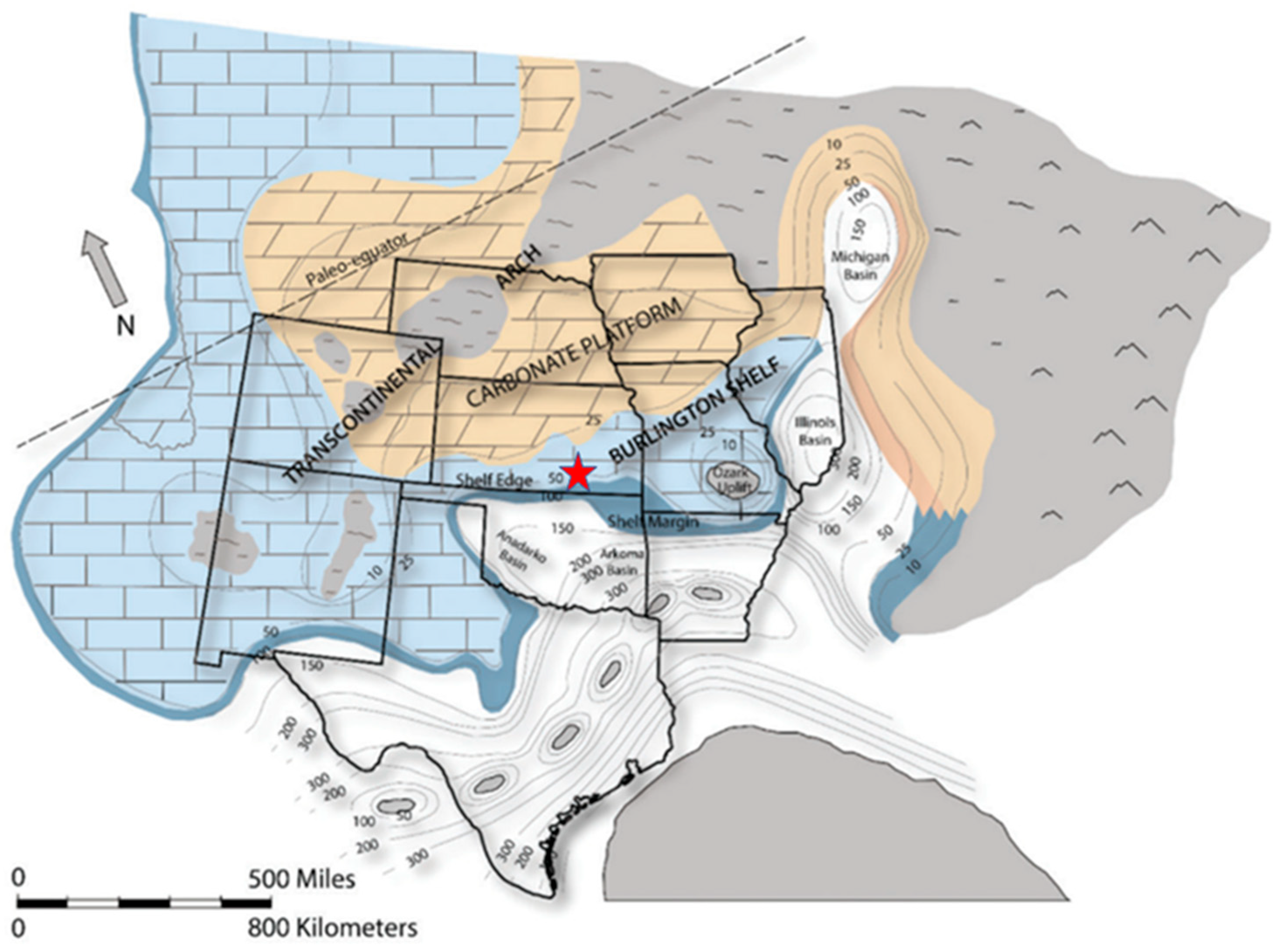
• A discernable boundary (marked by a black dashed line in Figure 22b) in the Wellington field part of the study area indicated the shelf edge, marking the transition from the carbonate shelf facies (region above the black line in Figure 22b) to the shelf margin facies (region below the black line in Figure 22b). This inference is consistent with the location of the study on the paleo-depositional model of the midcontinent portion of the Early Mississippian (Figure 1) [15].
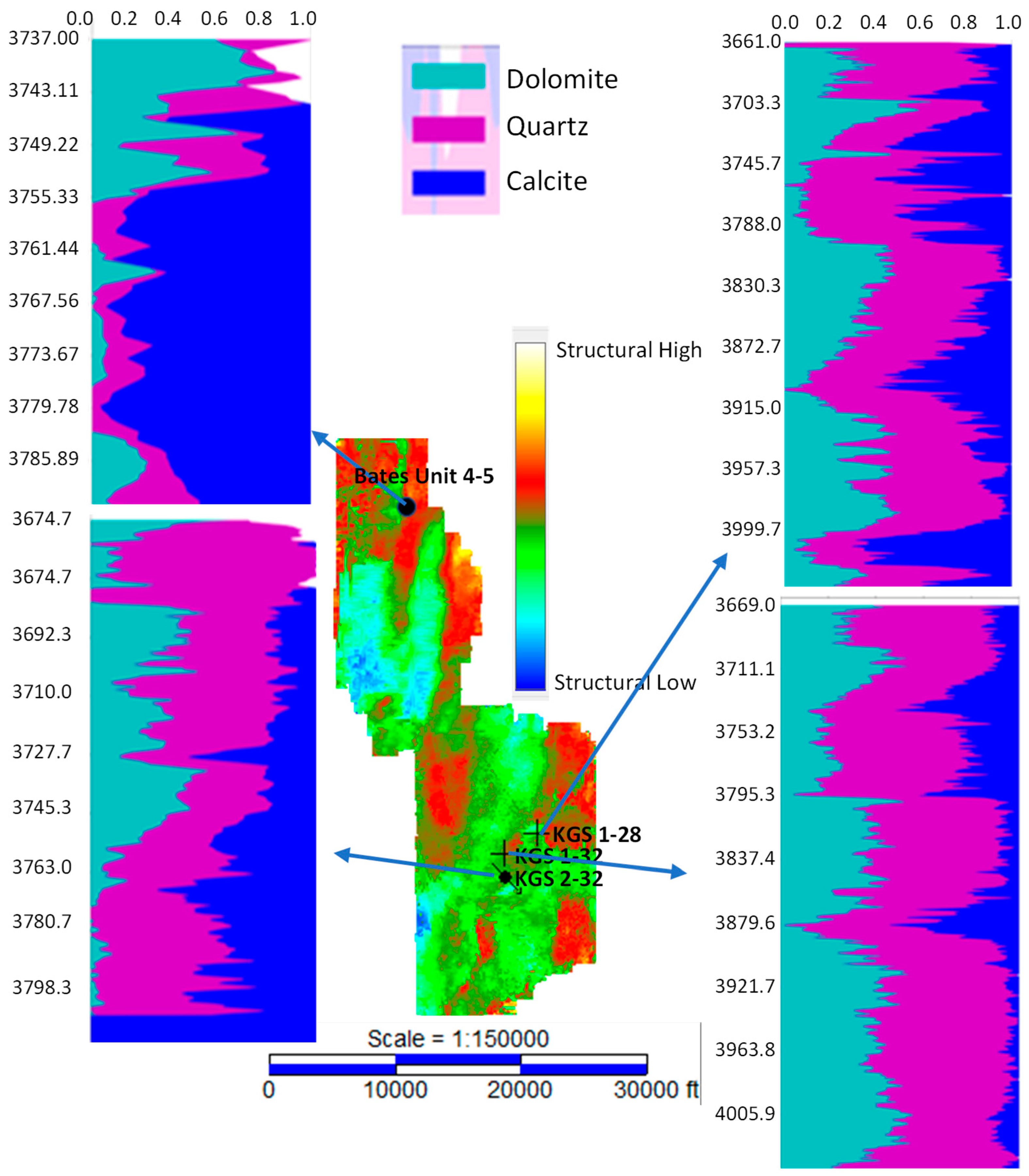
• From Figure 8, Well KGS 1-32 (c) has the highest combined dolomite and quartz average composition and penetrates facies F1 within the shelf region (Figure 22b). Well KGS 1-28(d) follows and penetrates facies F6 within the shelf margin region (Figure 22b). Well KGS 2-32(b) is next and penetrates facies F3 within the shelf margin region (Figure 22b). Lastly, Bates Unit 4–5 (a) also penetrates facies F3 within the shelf region (Figure 22b). Correlating these with the petrophysical facies model in Figure 22a revealed facies F1 had high porosity (Class 1). In contrast, facies F3 and F6 had low porosity (Class 3).
• Facies F4 is abundantly distributed in the shelf margin zone of the Wellington field part of the study area (Figure 22b). Most of it coincides with the medium porosity (class 2) facies, which tends to align with the lineament ‘N’ delineated in Figure 22a. In addition, the facies centroid Euclidean distance matrix shows facies F4 is closest to facies F3 (6 units) and F6 (6.2 units) (Figure 22c). Hence, the inference that facies F4 is a secondary petrophysical (porosity) facies generated by the reworking of facies F3 and F6 induced by the reactivation of the lineament ‘N.’
• Facies F1 and F2 (Figure 22b) coincide with high porosity (class 1) facies (Figure 22a). Moreover, from the distance matrix in Figure 22c, facies F1 and F2 are closest (4.9 units); hence, the inference of a possible high-porosity sub-class facies.
• Facies F5 is dominant in the Anson-Bates part of the shelf facies (Figure 22b). It coincides with both high-porosity (Class 1) facies and low-porosity facies (Class 3) in Figure 22a. Its facies centroid distance is far from the remaining facies (Figure 22c). Hence, the inference of a diagenetic facies with no petrophysical imprint within the reservoir. Facies F7 in the figure also shows distinctive facies within the F3 facies dominant in the Wellington field part of the shelf margin facies (Figure 22b). It trends roughly perpendicular (NW-SE) to the dominant trend of facies F3 (NE-SW) in which it is embedded. Its facies centroid distances are farthest from all the facies delineated (Figure 22c). Therefore, it could be an anomaly worth investigating to uncover further details.

Geological carbon sequestration has emerged as the most viable option of mitigating CO₂ emissions [39,40]. The broader geological sequestration options include depleted hydrocarbon reservoirs, where the target rock formation is a non-reservoir regional saline aquifer in a significant part of it, as is the case for the Mississippian and Arbuckle Formations of Kansas and Oklahoma [41,42]. The non-productive parts of such reservoirs are usually not characterized in sufficient detail or not characterized at all. Thus, seismic facies data that are productive and well-controlled pave the way for building viable rock formation facies models, which leverage the CO₂-injectore placements and in-depth understanding of the lithofacies controls on porosity and/or mineral trapping mechanisms. This project revealed the seismic facies variation based on a validated approach, which can be followed even in situations where the target formation is not well-penetrated by hydrocarbon-producing wells.

5. Conclusions

The seismic facies F1 and F2 correlate with porous zones in the study area. Judging by their relatively extensive lateral coverage, these facies represent the bulk properties that need to be considered in simulated CO₂ plume migration during EOR or direct geosequestration. The seismic facies delineated in this study are controlled by a complex blend of petrophysical (porosity), depositional, and diagenetic factors. However, the limitation of insufficient well core data for the wells made it challenging to determine the dominant factor on a particular seismic facies class. Furthermore, utilizing hierarchical analysis and K-means as two different distance-based clustering algorithms provided qualitative validation, additional to validation of the domain knowledge of carbonate depositional geometry. Multiple seismic facies clusters were deemed representative of the reservoir quality heterogeneity, which is controlled by litho-facies changes. Resolution enhancement and spectral decomposition improved and leveraged the data quality to aid in validation of the resulting facies boundaries. One of the impactful benefits of comparing hierarchical and K-means clustering methods is deducing the suitable number of clusters based on the hierarchical approach, which is revealing for the natural agglomeration of the input seismic attributes compared with the subjective data partitioning techniques, such as K-means clustering. This comparative methodology is unique to this study and enables the utilization of both the user-independent hierarchical clustering and the better-agglomerating data partition, K-means (e.g., Figure 10, Figure 11 and Figure 12).

Finally, to better understand the seismic facies controls and their effects on carbon storage, more core log data and mineral thin section analyses are recommended to be integrated into the study. This will leverage the lateral resolution strength of the seismic facies with the vertical resolution strength of core data analysis to produce a higher-resolution characterization of the reservoir.

References

1. O’Neill, S. Global CO2 Emissions Level Off in 2019, with a Drop Predicted in 2020. Engineering 2020, 6, 958–959. [Google Scholar] [CrossRef]
2. Bickle, M.J. Geological carbon storage. Nat. Geosci. 2009, 2, 815–818. [Google Scholar] [CrossRef]
3. Buchanan, R.; Carr, T.R. Kansas Geological Survey; University Press of Kansas: Lawrence, KS, USA, 1987; Volume 27, pp. 1–4. [Google Scholar]
4. Baines, S.J.; Worden, R.H. Geological storage of carbon dioxide. Geol. Soc. Spec. Publ. 2004, 233, 1–6. [Google Scholar] [CrossRef]
5. Shulakova, V.; Sarout, J.; Pimienta, L.; Lebedev, M.; Mayo, S.; Clennell, M.B.; Pervukhina, M. Effect of supercritical CO2 on carbonates: Savonnières sample case study. Geophys. Prospect. 2017, 65, 251–265. [Google Scholar] [CrossRef]
6. Siqueira, T.A.; Iglesias, R.S.; Ketzer, J.M. Carbon dioxide injection in carbonate reservoirs—A review of CO2-water-rock interaction studies. Greenh. Gases Sci. Technol. 2017, 7, 802–816. [Google Scholar] [CrossRef]
7. Tan, Y.; Li, Q.; Xu, L.; Ghaffar, A.; Zhou, X.; Li, P. A critical review of carbon dioxide enhanced oil recovery in carbonate reservoirs. Fuel 2022, 328, 125256. [Google Scholar] [CrossRef]
8. Masaferro, J.L.; Bourne, R.; Jauffred, J.-C. 3D visualization of carbonate reservoirs. Lead. Edge 2003, 22, 18–25. [Google Scholar] [CrossRef]
9. Bashir, Y.; Siddiqui, N.A.; Morib, D.L.; Babasafari, A.A.; Ali, S.H.; Imran, Q.S.; Karaman, A. Cohesive approach for determining porosity and P-impedance in carbonate rocks using seismic attributes and inversion analysis. J. Pet. Explor. Prod. Technol. 2024, 14, 1173–1187. [Google Scholar] [CrossRef]
10. de Mello, V.L.; Lupinacci, W.M. Mineralogy based classification of carbonate rocks using elastic parameters: A case study from Buzios Field. J. Pet. Sci. Eng. 2022, 209, 109962. [Google Scholar] [CrossRef]
11. Zhao, T.; Jayaram, V.; Roy, A.; Marfurt, K.J. A comparison of classification techniques for seismic facies recognition. Interpretation 2015, 3, SAE29–SAE58. [Google Scholar] [CrossRef]
12. Wrona, T.; Pan, I.; Gawthorpe, R.L.; Fossen, H. Seismic facies analysis using machine learning. Geophysics 2018, 83, O83–O95. [Google Scholar] [CrossRef]
13. Belyadi, H.; Haghighat, A. Unsupervised machine learning: Clustering algorithms. In Machine Learning Guide for Oil and Gas Using Python (Issue Ml); Elsevier: Amsterdam, The Netherlands, 2021. [Google Scholar] [CrossRef]
14. Hartigan, J.A. Statistical Clustering. In International Encyclopedia of the Social & Behavioral Sciences, 2nd ed.; Elsevier: Amsterdam, The Netherlands, 2015; pp. 392–396. [Google Scholar] [CrossRef]
15. Chopra, S.; Marfurt, K.J. Unsupervised Machine Learning Applications for Seismic Facies Classification. In Proceedings of the SPE/AAPG/SEG Unconventional Resources Technology Conference 2020, URTeC 2020, Virtual, 20–22 July 2020; pp. 1–8. [Google Scholar] [CrossRef]
16. Karakaya, S.; Ogiesoba, O.C.; Olariu, C.; Bhattacharya, S. Generating 3D lithology probability volumes using poststack inversion, probabilistic neural networks, and Bayesian classification—A case study from the mixed carbonate and siliciclastic deposits of the Cisco Group of the Eastern Shelf of the Permian Basin, north-central Texas. Geophysics 2024, 89, B131–B146. [Google Scholar]
17. Kruschke, J. Doing Bayesian Data Analysis: A Tutorial with R, JAGS, and Stan; Academic Press: Cambridge, MA, USA, 2014. [Google Scholar]
18. Wilson, E.N.; Watney, W.L.; Grammer, G.M. An Overview of the Giant Heterogeneous Mississippian Carbonate System of the Midcontinent: Ancient Structure, Complex Stratigraphy, Conventional Traps, and Unconventional Technology in a High Fluid Volume World. In AAPG Memoir; Grammer, G.M., Gregg, J.M., Pucket, J.O., Eds.; American Association of Petroleum Geologists: Tulsa, OK, USA, 2019; Volume 122, pp. 1–24. [Google Scholar] [CrossRef]
19. Wethington, N.W.; Pranter, M.J. Stratigraphic architecture of the Mississippian limestone through integrated electrofacies classification, Hardtner field area, Kansas and Oklahoma. Interpretation 2018, 6, T1095–T1115. [Google Scholar] [CrossRef]
20. Gutschick, R.C.; Sandberg, C.A. Mississippian continental margins of the conterminous United States. Shelfbreak Crit. Interface Cont. Margins 1983, 33, 79–96. [Google Scholar] [CrossRef]
21. Lane, H.R.; De Keyser, T.L. Paleogeography of the Late Early Mississippian (Tournaisian 3) in the central and southwestern United States. In Paleozoic Paleogeography of West-Central United States: Rocky Mountain Paleogeography Symposium 1; American Association of Petroleum Geologists: Tulsa, OK, USA, 1980; Volume 6, pp. 149–162. [Google Scholar]
22. Watney, W.L.; Guy, W.J.; Byrnes, A.P. Characterization of the mississippian chat in South-central Kansas. AAPG Bull. 2001, 85, 85–113. [Google Scholar] [CrossRef]
23. Montgomery, S.L.; Mullarkey, J.C.; Longman, M.W.; Colleary, W.M.; Rogers, J.P. Mississippian “Chat” Reservoirs, South Kansas: Low-Resistivity Pay in a Complex Chert Reservoir. AAPG Bull. 1998, 82, 187–205. [Google Scholar] [CrossRef]
24. Mazzullo, S.J.; Wilhite, B.W.; Boardman, D.R.; Morris, B.T.; Godwin, C.J. Lithostratigraphy, Biostratigraphy, Stratigraphic Architecture, and Depositional Systems in Lower to Middle Mississippian Strata on the Western Flank of the Ozark Dome, Midcontinent U.S.A. In Mississippian Reservoirs of the Midcontinent; American Association of Petroleum Geologists: Tulsa, OK, USA, 2019; pp. 25–57. [Google Scholar] [CrossRef]
25. Ohl, D.; Raef, A. Rock formation characterization for carbon dioxide geosequestration: 3D seismic amplitude and coherency anomalies, and seismic petrophysical facies classification, Wellington and Anson-Bates Fields, Kansas, USA. J. Appl. Geophys. 2014, 103, 221–231. [Google Scholar] [CrossRef]
26. Simm, R.; Bacon, M. Seismic Amplitude: An Interpreter’s Handbook; Cambridge University Press: Cambridge, UK, 2014; pp. 38–57. [Google Scholar]
27. White, R.E.; Simm, R. Tutorial: Good practice in well ties. First Break 2003, 21, 75–83. [Google Scholar] [CrossRef]
28. Walden, A.T.; White, R.E. On errors of fit and accuracy in matching synthetic seismograms and seismic traces. Geophys. Prospect. 1984, 32, 871–891. [Google Scholar] [CrossRef]
29. Karsli, H.; Dondurur, D. A procedure to reduce side lobes of reflection wavelets: A contribution to low frequency information. J. Appl. Geophys. 2013, 96, 107–118. [Google Scholar] [CrossRef]
30. Dowdell, B.L.; Kwiatkowski, J.T.; Marfurt, K.J. Seismic characterization of a Mississippi Lime resource play in Osage County, Oklahoma, USA. Interpretation 2013, 1, SB97–SB108. [Google Scholar] [CrossRef]
31. Verma, S.; Chopra, S.; Ha, T.; Li, F. A review of some amplitude-based seismic geometric attributes and their applications. Interpretation 2022, 10, B1–B12. [Google Scholar] [CrossRef]
32. Dewett, D.T.; Pigott, J.D.; Marfurt, K.J. A review of seismic attribute taxonomies, discussion of their historical use, and presentation of a seismic attribute communication framework using data analysis concepts. Interpretation 2021, 9, B39–B64. [Google Scholar] [CrossRef]
33. Oumarou, S.; Mabrouk, D.; Tabod, T.C.; Marcel, J.; Ngos, S., III; Essi, J.M.A.; Kamguia, J. Seismic attributes in reservoir characterization: An overview. Arab. J. Geosci. 2021, 14, 402. [Google Scholar] [CrossRef]
34. Macfarlane, P.A.; Doveton, J.H.; Coble, G. Interpretation of lithologies and depositional environments of Cretaceous and Lower Permian rocks by using a diverse suite of logs from a borehole in central Kansas. Geology 1989, 17, 303–306. [Google Scholar] [CrossRef]
35. Cohen-Addad, V.; Kanade, V.; Mallmann-Trenn, F.; Mathieu, C. Hierarchical clustering: Objective functions and algorithms. J. ACM (JACM) 2019, 66, 1–42. [Google Scholar] [CrossRef]
36. Strauss, T.; Von Maltitz, M.J. Generalising Ward’s method for use with Manhattan distances. PLoS ONE 2017, 12, e0168288. [Google Scholar] [CrossRef]
37. Dubey, A.; Choubey, A.P.D.A. A systematic review on k-means clustering techniques. Int. J. Sci. Res. Eng. Technol. (IJSRET) 2017, 6, 624–627. [Google Scholar]
38. Kodinariya, T.M.; Makwana, P.R. Review on determining number of Cluster in K-Means Clustering. Int. J. 2013, 1, 90–95. [Google Scholar]
39. Ali, M.; Jha, N.K.; Pal, N.; Keshavarz, A.; Hoteit, H.; Sarmadivaleh, M. Recent advances in carbon dioxide geological storage, experimental procedures, influencing parameters, and future outlook. Earth-Sci. Rev. 2022, 225, 103895. [Google Scholar] [CrossRef]
40. Ampomah, W.; Balch, R.; Will, R.; Cather, M.; Gunda, D.; Dai, Z. Co-optimization of CO2- EOR and Storage Processes under Geological Uncertainty. Energy Procedia 2017, 114, 6928–6941. [Google Scholar] [CrossRef]
41. Ganesh, P.R.; Mishra, S.; Haagsma, A.; Gupta, N. Dynamic modeling to understand pressure response from oil production and CO2 injection in a depleted pinnacle reef reservoir: Manual calibration using simplified resolution of reservoir heterogeneity. Int. J. Greenh. Gas Control 2021, 108, 103308. [Google Scholar] [CrossRef]
42. Dai, Z.; Middleton, R.; Viswanathan, H.; Fessenden-Rahn, J.; Bauman, J.; Pawar, R.; Lee, S.Y.; McPherson, B. An integrated framework for optimizing CO2 sequestration and enhanced oil recovery. Environ. Sci. Technol. Lett. 2014, 1, 49–54. [Google Scholar] [CrossRef]
Figure 1. Generalized static paleo-depositional model of the midcontinent showing principal tectonic elements during the Mississippian time, after Wilson et al. [18]. The red star marks Sumner County, Southcentral Kansas, where the study area is located.
Geosciences 15 00257 g001
Figure 2. Location of the state of Kansas on in relation to central and eastern U.S.A. (left), Geological map of the state of Kansas (right) showing the Mississippian strata and existing geological structures (the dotted lines marked A and B are significant basement lineaments) [19].
Geosciences 15 00257 g002
Figure 3. Generalized stratigraphy of the Mississippian system in Kansas [18]; the whole stratigraphic succession in Kansas can be found at https://www.kgs.ku.edu/General/Strat/Chart/ (accessed on 4 April 2025).
Geosciences 15 00257 g003
Figure 4. State of Kansas County map (right) and seismic Survey map (left) of the study area in Sumner County, Kansas; modified from Ohl and Raef [25].
Geosciences 15 00257 g004
Figure 5. (a) The seismic-to-well tie shows the Mississippian peak reflector (blue arrow) and (b) Synthetic 1D trace model (blue circle) with a correlation coefficient of 0.63 to seismic data trace (red circle).
Geosciences 15 00257 g005
Figure 6. Plot showing frequency bandwidths of the original amplitude spectrum 1 (blue) and spectral whitened amplitude spectra 2 (purple), 3 (orange), and 4 (green); spectrum 4 data were selected for seismic attribute extraction.
Geosciences 15 00257 g006
Figure 7. Seismic sections for the respective amplitude spectrums. The blue circle highlights a pinch-out feature progressively resolved due to the reduction in interference of thin beds as frequency bandwidth increases from the original spectrum 1 (a) through spectrum 2 (b) and 3 (c) to spectrum 4 (d).
Geosciences 15 00257 g007
Figure 8. Dolomite, quartz, and calcite mineral proportions for selected wells, which are plotted on a time structural map, of the Anson-Bates and Wellington field study area. The structurally lower Bates Unit 4–5 location targeted greater thickness of 10% or less dolomitization.
Geosciences 15 00257 g008
Figure 9. Grid model section showing the variability of reservoir quality within the Wellington field, the cross-section line map location; reservoir quality of good, moderate, poor, and tight is displayed with color-coded model facies.
Geosciences 15 00257 g009
Figure 10. Delineated seismic facies by hierarchical (H) and K-means (K) clustering for the original spectrum of the data; the clustering with K-means provided the number of clusters that can be used in the hierarchical dendrogram, i.e., the level of branching off to define meaningful clusters.
Geosciences 15 00257 g010
Figure 11. Delineated seismic facies by hierarchical (H) and K-means (K) clustering for the original spectrum at the 20 Hz frequency sub-band of the data; with 10 K-means facies clusters, the discrepancy between the two techniques is apparent.
Geosciences 15 00257 g011
Figure 12. Delineated seismic facies by hierarchical (H) and K-means (K) clustering for the original spectrum at 30 Hz frequency sub-band of the data.
Geosciences 15 00257 g012
Figure 13. Delineated seismic facies by hierarchical (H) and K-means (K) clustering for the original spectrum at 40 Hz frequency sub-band of the data.
Geosciences 15 00257 g013
Figure 14. Delineated seismic facies by hierarchical (H) and K-means (K) clustering for the original spectrum at 50 Hz frequency sub-band of the data.
Geosciences 15 00257 g014
Figure 15. Delineated seismic facies by hierarchical (H) and K-means (K) clustering for the original spectrum at composite 20–50 Hz frequency sub-band of the data.
Geosciences 15 00257 g015
Figure 16. Delineated seismic facies from original (O) and resolution-enhanced (S) spectrums at the entire frequency bandwidth of the data.
Geosciences 15 00257 g016
Figure 17. Delineated seismic facies from original (O) and resolution-enhanced (S) spectrums at 20 Hz frequency sub-band of the data.
Geosciences 15 00257 g017
Figure 18. Delineated seismic facies from original (O) and resolution-enhanced (S) spectrums at 30 Hz frequency sub-band of the data.
Geosciences 15 00257 g018
Figure 19. Delineated seismic facies from original (O) and resolution-enhanced (S) spectrums at 40 Hz frequency sub-band of the data.
Geosciences 15 00257 g019
Figure 20. Delineated seismic facies from original (O) and resolution-enhanced (S) spectrums at 50 Hz frequency sub-band of the data.
Geosciences 15 00257 g020
Figure 21. Delineated seismic facies from original (O) and resolution-enhanced (S) spectrums at composite 20–50 Hz frequency sub-band of the data.
Geosciences 15 00257 g021
Figure 22. (a) Petrophysical (porosity) facies map with delineated lineaments (black dashed lines) by Ohl & Raef [25], (b) seismic facies map with delineated shelf edge (black dashed line) and wells containing mineral proportion and reservoir quality data, and (c) Euclidean distance matrix for the centroids of seismic facies in (b) indicating non-similar seismic facies clusters.
Geosciences 15 00257 g022
Disclaimer/Publisher’s Note: The statements, opinions and data contained in all publications are solely those of the individual author(s) and contributor(s) and not of MDPI and/or the editor(s). MDPI and/or the editor(s) disclaim responsibility for any injury to people or property resulting from any ideas, methods, instructions or products referred to in the content.