Enhanced Gold Ore Classification: A Comparative Analysis of Machine Learning Techniques with Textural and Chemical Data

Abstract

Specific computational methods, such as machine learning algorithms, can assist mining professionals in quickly and consistently identifying and addressing classification issues related to mineralized horizons, as well as uncovering key variables that impact predictive outcomes, many of which were previously difficult to observe. The integration of numerical and categorical variables, which are part of a dataset for defining ore grades, is part of the daily routine of professionals who obtain the data and manipulate the various phases of analysis in a mining project. Several supervised and unsupervised machine learning methods and applications integrate a wide variety of algorithms that aim at the efficient recognition of patterns and similarities and the ability to make accurate and assertive decisions. The objective of this study is the classification of gold ore or gangue through supervised machine learning methods using numerical variables represented by grade and categorical variables obtained through drillholes descriptions. Four groups of variables were selected with different variable configurations. The application of classification algorithms to different groups of variables aimed to observe the variables of importance and the impact of each one on the classification, in addition to testing the best algorithm in terms of accuracy and precision. The datasets were subjected to training, validation, and testing using the decision tree, random forest, Adaboost, XGBoost, and logistic regression methods. The evaluation was randomly divided into training (60%) and testing (40%) with 10-fold cross-validation. The results revealed that the XGBoost algorithm obtained the best performance, with an accuracy of 0.96 for scenario C1. In the SHAP analysis, the variable As was prominent in the predictions, mainly in scenarios C1 and C3. The arsenic class (Class_As), present mainly in scenario C4, had a significant positive weight in the classification. In the Receiver Operating Characteristic (ROC) and Area Under the Curve (AUC) curves, the results showed that XGBoost/scenario C1 obtained the highest AUC of 0.985, indicating that the algorithm had the best performance in ore/gangue classification of the sample set. The logistic regression algorithm together with AdaBoost had the worst performance, also varying between scenarios.

1. Introduction

In mining operations, different types of materials, whether ore or gangue, are mapped and sampled, prior to being analyzed and characterized by a wide variety of analytical and descriptive techniques for industrial processing or research purposes. Typically, these samples are characterized to constitute a large database with thousands of different items of information that can be used in predictions at various stages of mineral evaluation.

One of the main objectives of process mineralogy is related to the study of the aspects of geological materials and their mineral associations that can directly assist in determining the characteristics of ore bodies, their recovery potential, and behavior in mineral processing. Descriptive analyses, such as of drill cores, and their characteristics such as alteration, roughness, sulfidation, hardness, or even predominance of minerals of interest, are also inserted into geological databases and used in mineral evaluations such as resource estimates [1,2]. A well-executed characterization of the materials to be processed can provide insights for more efficient and optimized mineral operations, maximizing potential gains in the beneficiation process [3,4,5]. Integrated data, including grade and detailed descriptions of geological materials, are commonly used in studies to define mineralized layers of interest [6,7]; they can also offer additional information, such as concerning temporal relationships and the mineralization environment.

A textural analysis of various geological materials can reveal patterns that reflect a characteristic spatial arrangement of minerals [8,9,10]. These patterns are typically associated with human visual perception in a geological context, relating to intrinsic material characteristics such as mineral associations, boudinage quantification and deformation, sulfidation, and other features. Textural analysis can be performed through mathematical representations, either quantitative or qualitative, of a sample or sample interval [11,12], and may implicitly contain valuable information regarding the geological conditions of the deposit.

One of the main challenges in developing a systematic textural classification is its standardization, as the traditional understanding of different rock textures and structures is primarily descriptive, intuitive, and rooted in a human-centered language that categorizes qualitative and quantitative features in distinct ways [13]. In this context, automation remains limited in its application of mathematical models, as the current framework of machine learning algorithms cannot fully capture the depth of human experience and insights. However, many classification, regression, and clustering algorithms work by measuring the similarity between observations in an n-dimensional space to define and label clusters or features, using both categorical and numerical data [14]. Categorical variables are often descriptive and can assume a range of limited numerical values that represent the predominant qualitative characteristics of an analyzed space. Examples of categorical variables may be lithology, degree of alteration, deformation, or types of mineralization [15,16]. Categorical variables can be divided into ordinal variables, which have a natural ordering into categories, such as high, medium, or low, and nominal variables, which do not have an intrinsic ordering into categories, such as lithology.

In a database with analytical information, represented by information and descriptive data on geological materials together with categorical information, the application of Artificial Intelligence (AI), and particularly machine learning (ML), contributes significantly to the analysis and integration of data, showing relationships between variables and patterns that were not observed or were difficult to observe. ML is a discipline of computer science that focuses on the study of mathematical models using a structured database in the prediction of a variable of interest or in the classification from a dataset [17,18,19]. The validated database is the central part of any prediction system, automated classification, regression tasks, clustering, and association rule learning. Machine learning can adopt new methods according to the input characteristics, simulate human learning methods, or combine several mathematical models [20].

The application of mathematical models can be categorized into four main architectures depending on the type of desired output or learning: supervised [21], unsupervised [22,23], semi-supervised [24], and reinforcement learning [25]. Learning refers to a set of procedures defined to adjust the parameters of an AI model, so that it can learn a certain function. One of the main advantages of using machine learning models is their ability to deal with additive variables, which is a mathematical property that allows the calculation of the average of a variable through linear averaging [26,27], generating a result with the same property as the input samples. Some process parameters are not necessarily additive [28]; for example, metallurgical recoveries represent the percentage of the metal of interest that is recovered in the product, reagent yield in a flotation step, abrasiveness index, etc. The most common solutions to treat non-additive variables are the application of geostatistical methods using conditional simulation [29,30], sensitivity analysis that evaluates how a variable can influence the others, and decorrelation using Principal Component Analysis and machine learning models based on decision trees [31,32,33,34].

Regarding mineral characterization and the application of ML algorithms, recent publications have been produced focusing mainly on a framework based on classification algorithms for recovery and optimization of reagent yield [35] and regression methods applied to different types of ores in the prediction of variables of operational importance. ML has focused on prediction by applying specific learning algorithms to observe similarity patterns in large databases [36].

The performance of algorithms has been the subject of several studies in the prediction of geological variables. Ref. [37] published a review on the applications of machine learning in mineral processing. Variables obtained from mineralogical characterization of gold ore, such as arsenic content, gold, as well as mineral assemblages, and gold grain size influence the accessibility of the leach solution and the recovery of gold [38,39]. Ref. [40] developed a methodology to integrate process properties into a spatial model using machine learning methods and compared performance across six properties such as iron recovery, Davis tube mass traction, low-intensity wet magnetic separation, release of iron oxides, and P₈₀.

This study aims to improve the classification process of mineralized zones classified as ore and gangue based on chemical and textural variables that were analyzed using supervised learning. The study explores five different scenarios to assess the significance and impact of various variables on machine learning models. The algorithms under consideration include decision tree (DT), random forest (RF), AdaBoost (Adaboost), Extreme Gradient Boost (XGBoost), and logistic regression (LR). After the model testing phase, the SHapley Additive exPlanations (SHAP) method is employed to improve the interpretability of the best performing model [41]. Python packages (version 3.11.13) along with libraries such as pandas, scikit-learn, NumPy, and SHAP, are utilized to conduct the required computations. Details of the algorithms and the steps involved in model development are presented in the subsequent sections, followed by results and discussion. Receiver Operating Characteristic (ROC) and Area Under the Curve (AUC) curves were also used to evaluate the classification performance of the model in various settings along with the confusion matrix. Accuracy is expressed as mean squared error (MSE).

2. Conceptual Framework

2.1. Evaluation and Validation

One of the parameters used to evaluate model performance was the mean squared error (MSE). This metric measures the mean of the squared errors; that is, it evaluates the mean squared difference between the observed and predicted values [42]. One possible interpretation is that the metric is sensitive to extreme values, as it squares the differences, making outliers more expressive. When a model has low errors, the MSE approaches zero. As the model error increases, its value increases (Equation (1)). The MSE can be used to compare different models where the model with the lowest MSE is generally considered the best fit in terms of accuracy. The formula for MSE is as follows:

$$\mathit{MSE}={\displaystyle \frac{\sum {\left(y_i-{\widehat{y}}_i\right)}^2}{n}}$$

(1)

$y_i$ = the $i$th observed value.

${\widehat{y}}_i$ = the corresponding predicted value.

$n$ = the number of observations.

Another metric used to evaluate model performance is precision, which is calculated by dividing the true positive values by the sum of true positive (TP) and false positive (FP) values [43], which is represented by (Equation (2)). Recall measures the frequency with which a model correctly identifies and provides the number of correct positive results. Equation (3) presents the recall calculation.

$$\mathit{Precision}={\displaystyle \frac{TP}{TP+FP}}$$

(2)

$$\mathit{Recall}={\displaystyle \frac{TP}{TP+FN}}$$

(3)

$TP$ = True positive.

$FP$ = False positive.

$FN$ = False negative.

The cross-validation method is used to evaluate data performance through modeling results evaluated using k-fold cross-validation with 10 folds. This method involves randomly dividing the original dataset into k subsets of the same size [21]. In this procedure, the data processing is iterated k times, ensuring that all partitions are trained and tested. Classification metrics, including precision, accuracy, and recall, can be applied. This approach allows a complete evaluation of the available data, providing accurate classification while considering the various data formation and clustering characteristics.

Another form of representation, the confusion matrix, shows in a binary form real values and predicted values that help in the visualization and interpretation of a classifier’s performance [43,44]. In this binary classification, there are usually two target classes labeled as “positive” and “negative” or “1” and “0”. The main diagonal of the confusion matrix represents the accuracy of the evaluated records, consolidating the true results in an organized way within the matrix. Figure 1 shows the confusion matrix.

ROC curves and AUC are widely used to evaluate the classification performance of an ML model at various threshold settings. The ROC curve is represented as a graph and represents the TP and FP rate at different thresholds. The curve shows how the sensitivity and specificity of the model change as the classification thresholds are changed. The closer the curve is to the upper left corner of the graph, the better the model is performing. AUC is a measure of the area under a ROC curve analysis. It provides a single measure of model performance, with AUC = 1 showing a perfect model that classifies all positives and negatives correctly. AUC < 0.5 represents poor model performance, indicating randomness in prediction.

2.2. Machine Learning Methods for Ore Classification

2.2.1. Decision Tree (DT)

Decision tree is a supervised learning algorithm with a hierarchical tree structure with a high level of performance, which can be applied in multivariate classification and regression in prediction using large volumes of data and which is structured in the form of nodes and leaves [45,46,47,48].

Decision Tree Algorithms can be applied in a variety of cases with some advantages such as easy interpretation and visualization due to their hierarchical nature, not requiring data normalization, and being able to work with various types of integrated data, such as categorical and numerical data, as well as missing data. However, their disadvantages are capturing noise (overfitting) and difficulty in processing more complex data.

2.2.2. Random Forest (RF)

Random forest (RF) is a nonparametric supervised method that combines multiple decision trees to improve the accuracy and robustness of predictions [49].

The method averages its results by incorporating random subspaces and can effectively reduce the impact of less significant features based on their importance [50,51]. One of the advantages of applying the RF method is accuracy; it is less prone to overfitting because the average of predictions reduces the variance. The disadvantages are the training time and memory consumption. The following equation (Equation (4)) summarizes the RF operator where $\left(x\right)$ denotes input and $\widehat{T}\left(x\right)$ is the estimation produced by the $k\mathrm{th}$ tree.

$$\widehat{T}\left(x\right)={\displaystyle \frac{1}{k}}{{\displaystyle \sum }}_{k=1}^k\widehat{T_K}\left(X\right)$$

(4)

2.2.3. AdaBoost

The core principle of AdaBoost is to fit a sequence of weak learners (i.e., models that are only slightly better than random guessing, such as small decision trees) on repeatedly modified versions of the data. The predictions from all of them are then combined through a weighted majority vote (or sum) to produce the final prediction. The data modifications at each so-called boosting iteration consists of applying weights [52].

In the initial phase, the algorithm works by building a model using the training dataset, and then a second model is created to correct the errors made by the first model. This process continues until the errors are minimized and the dataset is predicted with greater accuracy. AdaBoost algorithms operate in a similar manner, as they combine multiple models to produce a more robust final result. Although the algorithm is sensitive to noise and outliers, it is less prone to overfitting compared to other algorithms.

2.2.4. Extreme Gradient Boost (XGBoost)

Extreme Gradient Boost (XGBoost) is a tree-based ensemble method that employs a gradient-boosting framework. It combines multiple weak regression trees and iteratively merges their predictions to increase accuracy by correcting the errors of the previous trees [19,53].

The learning process involves constructing decision trees that sequentially reduce the loss function following the direction of the gradient [54]. Gradient-boosting trees in XGBoost typically consist of short decision trees with high bias but low variance and can handle missing data. The main goal of boosting in XGBoost is to reduce bias, although it can also effectively address variance.

2.2.5. Logistic Regression (LR)

The logistic regression algorithm is a supervised classifier based on regression rules that models the probability of a binary dependent variable; that is, one that assumes only two values (0 or 1). This probability represents a given input belonging to one of two predefined categories.

The fundamental principle of regression lies in the ability of the logistic function to accurately model the probability of binary outcomes. The characteristic S-shaped curve of the sigmoid function allows it to efficiently map any real-value input to a value between 0 and 1. This property makes logistic regression particularly effective for binary classification tasks, where the goal is to classify input data into one of two categories, such as determining and classifying it as “ore” or “non-ore” [55].

2.3. Shapley Additive exPlanations

The Shapley Additive exPlanations (SHAP) method is an ML model interpretation technique that takes a game-theoretic approach and aims to quantify the marginal effects of individual features and the interaction effects of pairs of features to explain the predictions made by any ML model [56,57].

SHAP works by dividing the output of a model into the contributions of each feature. It calculates a value that represents the impact of each feature on the model’s prediction result. These values are beneficial for understanding feature importance, interpreting model predictions, and assessing the local relevance of features using sample data instances from the dataset.

SHAP assigns a score, known as a SHAP value, to each feature to indicate its importance in influencing the model output and adheres to several key properties, including local accuracy, absence, consistency, and symmetry [58,59,60]. Local accuracy ensures that the explanations provided by SHAP align with the behavior of the original model. Consistency ensures that the attribution to a variable will not decrease, even if the model is adjusted to increase the impact of that variable. Symmetry ensures that if two features contribute equally to the prediction, they are assigned the same SHAP value.

By defining the output of a model, a more comprehensive understanding of the contributions of features and their impact on the model predictions can be achieved. SHAP defines the output of a model as follows (Equation (5)):

$$f\left(x\right)=g\left(z^{\prime }\right)={\varnothing }_0+{\sum }_{i=1}^m{\varnothing }_i{z}_i^{\prime }$$

(5)

$g\left(z^{\prime }\right)=$ SHAP explanation model.

${\varnothing }_0=$ SHAP value.

$z_i^{\prime }=$ binary variable.

3. Materials and Methods

3.1. Dataset Description

The dataset is composed of 16,826 intervals of 1 m in length obtained by core sampling. The chemical analysis was carried out by fire assay to determine Au content, while As, Pb, Zn, and Cu were analyzed by ICP-OES and S by the pyrolysis method in an induction furnace with determination by infrared cell. The mineralization is typically composed of sulphide refractory gold ore and was provided by a low-grade-gold-producing company (<0.6 g/t). The deposit was hosted in carbonaceous sericitic phyllite with the intercalation of phyllosilicate, essentially composed of chlorite, and millimeter quartzite lenses, centimeter-sized boudins, and veinlets associated with sulfides. These sulfides, in general, are represented by pyrite, arsenopyrite, and sparse occurrences of pyrrhotite, sphalerite, chalcopyrite, and galena. Gold grains essentially occur associated with sulfides, mainly in arsenopyrite and pyrite, with few free gold grains.

These three elements (As, Au, and S) are crucial in delineating the mineralized zones, as their relationships indicate the potential for gold mineralization. According to the study in [38], gold is associated with these elements, and there is a direct relationship between arsenic and gold, due to the mineral association between gold particles and arsenopyrite.

A total of 16 input variables were analyzed, comprising 7 numerical variables derived from chemical assays and 9 categorical variables obtained through descriptive analysis of drill cores. The categorical features used in the study are summarized in

Table 1. Description of the categorical variables inputted at the model.

#	Variable	Parameters	Categorical Variable Description
1	Class_Boud	L ≤ 20 boudings; M = 21–40; H ≥ 41	Occurrences of stretched quartz bands. High occurrence indicates a greater potential for the presence of sulfides.
2	Au_Potenc	L ≤ 29 units; M = 30–5; H ≥ 50	Gold potential is a sum of quartz boudins, deformation and occurrence of sulfide.
3	Class_As	L ≤ 2 clusters; M = 3–6; H ≥ 7	Occurrence of clusters with a predominance of arsenopyrite.
4	Class_Hardn	L ≤ 6.9 kWh/t; M = 7–11.9H ≥ 12	Material hardness is classified due to limitations in grinding efficiency when it falls outside the mill’s specifications.
5	Class_Def	L ≤ 5 deformed; M = 6–10; H ≥ 11	Greater deformation increases the potential for sulfide accumulation. Indicated by the presence of microfolds.
6	Sulfetac	L ≤ 5 clusters; M = 6–15; H ≥ 16	Occurrence of sulfides either in the form of clusters or dissemination in the samples.
7	Class_Silic	L ≤ 3% visual qtzo; M = 4–10; H ≥ 11	Silicate minerals, such as quartz, indicates lower sulfidation potential.
8	Class_Text	L ≤ 0.1 cm; M = 0.2–1; H ≥1.1	Potential indicator of mineralization in relation to grain size.
9	Class_Pb-Zn	L = 10 clusters; M = 11–30; H ≥ 31	Presence of sphalerite and galena.

.

The dataset was split into 60% for training and 40% for testing. A 10-fold cross-validation was performed within the training subset to fine-tune hyperparameters and evaluate model stability. After identifying the optimal configurations, each model was retrained using the full training data. The test set, kept completely separate throughout the process, was used exclusively for the final evaluation, ensuring an unbiased assessment. According to the study in [38], gold was associated.

3.2. Framework

The structure of the study involved compiling a dataset with chemical analyses and textural and genetic characteristics of gold zones through detailed geological descriptions. This dataset was subjected to classification using machine learning (ML) algorithms across different scenarios, with performance evaluated using four distinct models. Figure 2 illustrates the flowchart of activities and procedures based on the adopted methodology.

During the data preparation and preprocessing stage, quality control was performed, instances with missing values were removed, and outliers were identified. Data processing and model training were conducted using Python packages, including NumPy [61], pandas [62], scikit-learn [63], matplotlib [64], and seaborn (version 0.9.0). Various combinations of training and testing sets were used to optimize model hyperparameters for improved accuracy.

Table 2. Description of the hyperparameters for each ML model.

Model	Hyperparameters	Grid Search Range
DT	max_depth	3–10
	min_samples_split	2–4
	min_samples_leaf	1–4
	random_state	0–200
RF	number of estimators	100–300
	max_depth	1–10
	max_features	‘sqrt’, ‘log2’, ‘None’
	random_state	0–100
AdaBoost	number of estimators	1–200
	base estimator	tree
	learning_rate	1–0.001
	random_state	0–100
	algorithm	‘’sammer.r’
XGBoost	number of estimators	100–200
	max_depth	3–10
	learning_rate	1–0.01
	gamma	0–0.5
	base estimator	tree
LR	C	0.01–1000
	penalty	L1, L2
	Solver	lbfgs
	maximum iterations	1000

presents the main parameters adjusted for each ML algorithm.

Following validation and descriptive statistical analysis, input variables were standardized so that each feature had a mean of zero and a standard deviation of one. Standardization is essential as many ML algorithms are sensitive to input data scale; variables with larger ranges may dominate model learning and obscure meaningful patterns.

Table 3. Characterization of 16 variables inputted for ML modeling.

#	Input Variable	Variable Description	Unit	Scenario
				1	2	3	4
1	Au	Gold grade	g/t	x	x
2	As	Arsenic grade	g/t	x		x
3	S	Sulfur grade	%	x	x
4	Class_Boud	Boudinage, being 1 = L; 2 = M; 3 = H	cat	x	x	x	x
5	Au_Potenc	Au potential, being 1 = L; 2 = M; 3 = H	cat	x		x	x
6	Class_As	As potential, being 1 = L; 2 = M; 3 = H	cat	x		x	x
7	Class_Hardn	Hardness, being 1 = L; 2 = M; 3 = H	cat	x	x	x	x
8	Class_Def	Deformation, being 1 = L; 2 = M; 3 = H	cat	x	x	x	x
9	Sulfetac	Sulfidation, being 1 = L; 2 = M; 3 = H	cat	x	x		x
10	Class_Silic	Silicification, being 1 = L; 2 = M; 3 = H	cat	x	x	x	x
11	Class_Text	Texture, being 1 = L; 2 = M; 3 = H	cat	x	x	x	x
12	MAG	Magnetic susceptibility	num	x	x	x	x
13	Class_Pb-Zn	Pb-Zn, being 1 = L; 2 = H	cat	x	x	x	x
14	Pb	Lead grade	ppm	x	x		x
15	Zn	Zinc grade	ppm	x	x		x
16	Cu	Copper grade	ppm	x	x		x

x: selected variable L: low; M: Medium; H: High; num: numerical; cat: categorical.

describes four classification scenarios, selected to evaluate the influence of specific variables in distinguishing between ore and gangue. While qualitative assessments alone are insufficient to define mineralized zones, their contribution to identifying such zones and guiding subsequent beneficiation processes was considered in the scenario definitions.

To facilitate interpretation, the four scenarios can be summarized as follows: Scenario C1 includes all 16 input variables, serving as a comprehensive baseline. Scenario C2 excludes both arsenic grade (As) and its categorical counterpart (Class_As), as well as the variable representing gold potential (Au_Potenc), to assess model performance without key geochemical indicators. Scenario C3 removes the main metallic elements (Au, S, Pb, Zn, and Cu), isolating the influence of textural and categorical features. Scenario C4 maintains the frequency-based variable Class_As while excluding the arsenic and gold grades, allowing an evaluation of the predictive power of descriptive arsenopyrite occurrence in the absence of assay data. This design allows testing of model robustness across different input configurations and operational constraints.

4. Results

4.1. Database

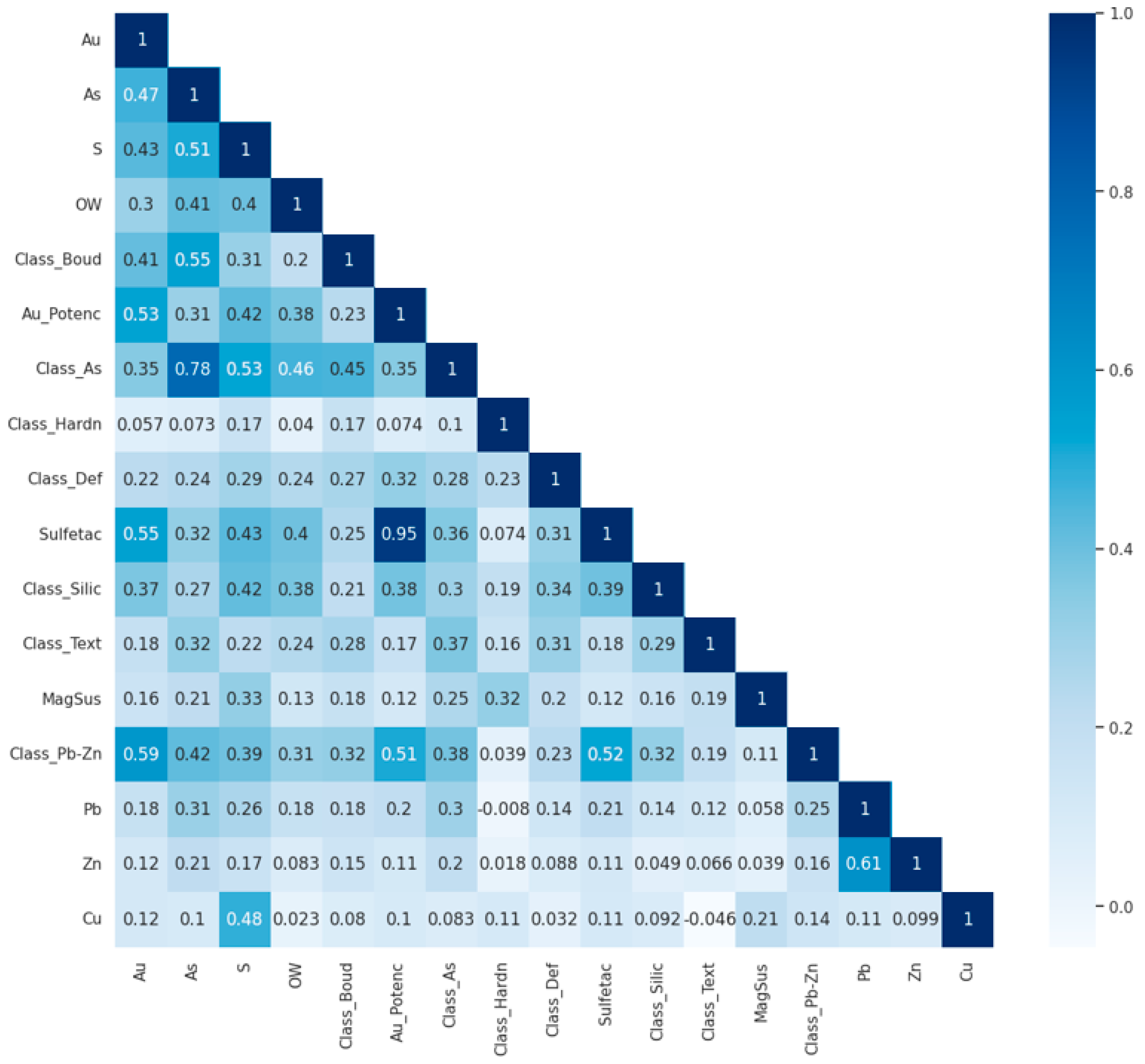
A correlation matrix was used to evaluate the relationships between the chemical and textural variables employed in the classification models (Figure 3). Categorical variables were ordinally encoded based on geological criteria—for example, frequency-based classes such as boudinage occurrence, arsenopyrite clusters, and sulfidation were classified into Low (1), Medium (2), and High (3). Although Pearson correlation was applied to both numerical and encoded categorical variables, it is important to emphasize that the matrix serves as an exploratory tool. The results should be interpreted with caution, especially for ordinal variables, as Pearson correlation assumes linear relationships and interval-scale data.

Despite this limitation, the matrix allows the visualization of general patterns and interactions among variables. A strong correlation (r = 0.95) was observed between the occurrence of sulfide clusters (Sulfetac), mainly composed of arsenopyrite and pyrite, and the variable representing the potential for gold occurrence (Au_Potenc). This relationship is consistent with the nature of refractory gold ores, where gold is often associated with sulfides, leading to lower recovery rates and the need for more complex processing techniques. Moderate correlations, between 0.5 and 0.7, occur between Pb and Zn classes (Class_Pb-Zn), such as secondary occurrences of galena and sphalerite, sulfidation, and potential occurrence of gold grains. Grade variables such as Au, As, and S are moderately to highly directly correlated with the arsenic class (Class_As), sulfidation, and Class_Boud due to the occurrence of boudins or sulfide clusters (essentially pyrite, arsenopyrite, chalcopyrite, and pyrrhotite) as a covering of these boudins. Another important correlation is the definition between ore and gangue; as expected, they are moderately associated with the contents, but with a significant contribution from the arsenic class, silicification, and potential for the occurrence of gold grains (Au_Potenc).

The As variable is a variable that controls mineralization together with the Au grade. Ref. [65] discussed the direct relationship between the mineral association of gold particles and arsenic content, along with an increase in the association with arsenopyrite and gold accessibility. However, very low relationships were observed between the Pb, Zn, and Cu content and hardness classes (Class_Hardn) and deformation classes (Class_Def).

The statistical analysis of the dataset is presented in

Table 4. Descriptive Statistics and Frequency Distribution of Variables Used in ML Modeling.

		Variables for Training Before Preprocessing					Variables for Training After Preprocessing
Variables	Unit	Mean	Stdev	Min	Median	Max	Mean	Stdev	Min	Median	Max
Au	g/t	0.405	0.361	0.01	0.32	4.58	1.9 × 108	1.0	1.1	−0.23	11.6
As	g/t	1543	1480	2.0	1098	9960	3.4 × 109	1.0	1.0	−0.30	5.75
S	%	0.94	0.372	0.1	0.9	3.13	1.1 × 108	1.0	2.2	−0.12	5.83
MAG		0.799	0.818	0.01	0.50	6.3	1.3 × 108	1.0	0.9	−0.37	6.71
Pb	ppm	59.1	123.2	1.01	23.0	2019	2.8 × 108	1.0	0.4	−0.29	15.9
Zn	ppm	96.9	110.6	1.02	76.0	2161	4.5 × 10	1.0	0.8	−0.19	18.7
Cu	ppm	38.6	12.1	0.26	37.1	150	5.0 × 109	1.0	3.1	−0.13	9.15
Frequency (%)
	Low	Med	High
Class_Boud	50.9	26.9	22.2
Au_Potenc	38.7	28.8	32.5
Class_As	44.4	31.6	24.0
Class_Hard	13.6	14.8	71.6
Class_Def	53.1	40.0	7.0
Sulfetac	39.3	27.2	33.4
Class_Silic	29.7	14.7	55.6
Class_Text	51.2	33.0	15.8
Class_Pb-Zn	59.8	-	40.2

, showing the statistics before and after standardization and frequency percentage for the categorical variables boudinage class, potential occurrence of gold based on sulfide agglomerations, occurrence of arsenopyrite particles, hardness having as a parameter whether it is friable or not, deformation, sulfidation, silicification, texture, and occurrence of secondary sulfides such as galena, pyrrhotite, and sphalerite (Class_Pb-Zn).

Standardization is a feature scaling method in which data values are rescaled to fit a distribution between 0 and 1 using mean and standard deviation as a basis for finding specific values. This operation ensures that different features have a similar contribution to machine learning models, preventing variables with different scales influencing the output results.

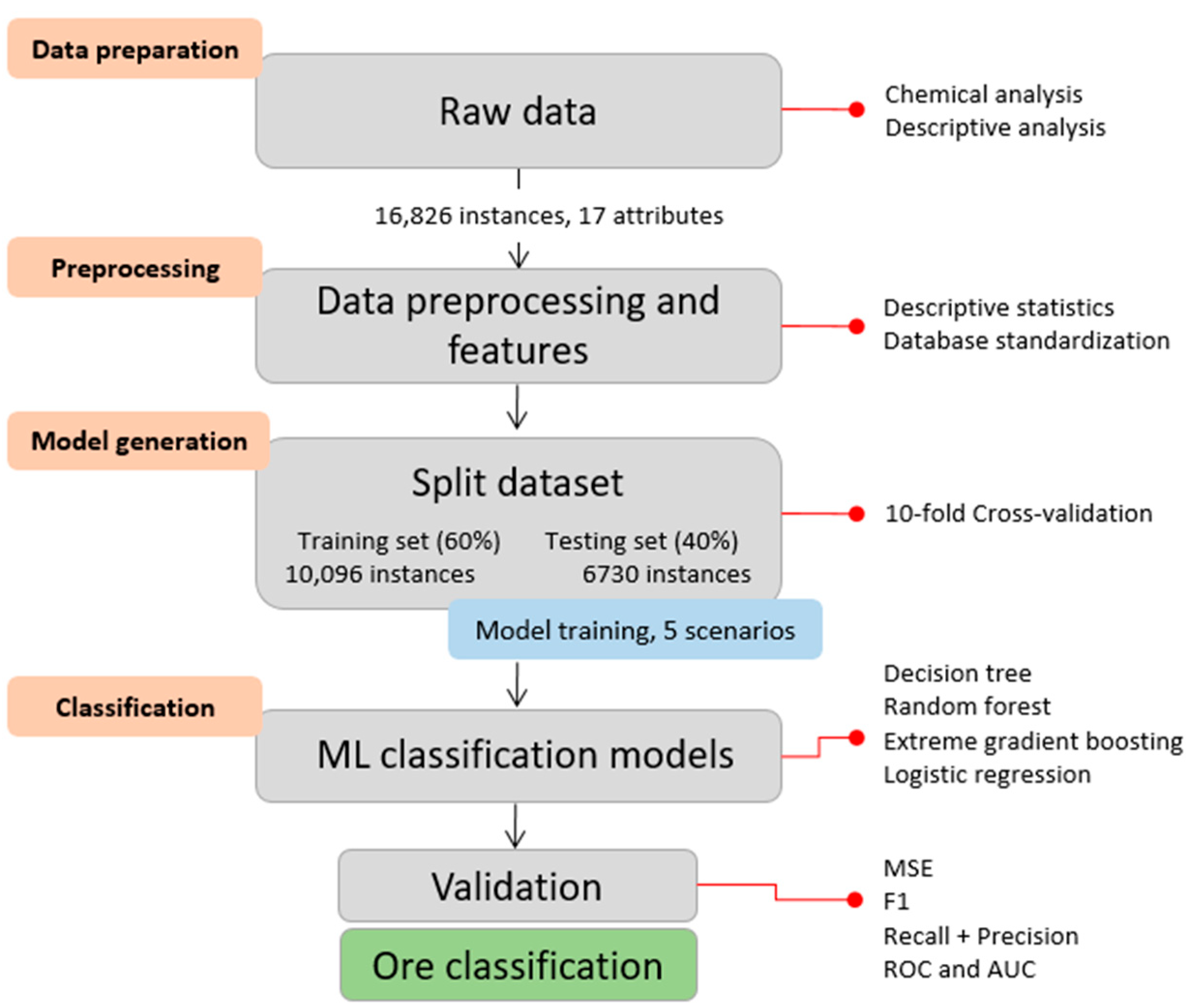
The hyperparameters for each supervised model tested to classify ore and gangue in the four selected scenarios are summarized in

Table 5. Different scenarios used for the model.

Model	Hyperparameters	Scenario C1	Scenario C2	Scenario C3	Scenario C4
DT	max_depth	6	10	6	6
	min_samples_split	2	3	2	2
	min_samples_leaf	1	1	2	1
	random_state	200	200	0	200
RF	num. of estimators	200	300	200	200
	max_depth	10	10	7	10
	max_features	sqrt	sqrt	sqrt	sqrt
	random_state	50	0	0	50
AdaBoost	num. of estimators	100	200	100	200
	base estimator	tree	tree	tree	tree
	max_depth
	learning rate	0.1	0.1	0.1	1
	random_state	0	0	0	0
	algorithm	samme	samme	samme	samme
XGBoost	num. of estimators	100	100	100	100
	max_depth	7	9	7	5
	learning_rate	0.1	0.1	0.1	0.1
	gamma	0	0.4	0.4	0.1
	base estimator	tree	tree	tree	tree
LR	C	0.01	100	0.01	0.1
	penalty	L2	L2	L2	L2
	Solver	lbfgs	lbfgs	lbfgs	lbfgs
	max_iterations	1000	1000	1000	1000

. The optimal hyperparameters for ensemble learners (AdaBoost, XGBoost, RF, and DT) are typically composed of a tree-based estimator, with a wide range of learning rates and number of estimators (trees), among the scenarios constructed.

Considering the tree estimator hyperparameter for the four models, the RF presented a higher number of estimators, mainly in scenario 2, with a reduction in the other scenarios. Similar behavior occurred with the AdaBoost, XGBoost, and DT models, with estimators of around 100. An exception can be observed in scenarios 2 and 4 for the AdaBoost model.

Another hyperparameter that presented low variation was the learning rate. The models presented around 0.1 with the exception of the AdaBoost model, which presented a rate varying to 1.

The “max depth” in ML refers to the parameter that limits the maximum depth based on DT estimators. The variation in values means that the model will not perform more divisions beyond this limit, helping to avoid overfitting and excessive model complexity. The value for the maximum depth can significantly impact the model’s performance. Different values were found between 5 and 10 throughout, with lower values for the DT model for scenarios 1, 3, and 4 and scenario 4 for the XGBoost algorithm.

To evaluate the performance of the algorithm, a 10-fold cross-validation was employed to obtain a generalized model that does not overfit on training data. In the cross-validation of the training, the original samples were randomly partitioned into ten equal-sized subsets. One subset was selected as the validation set for testing the model, while the remaining nine subsets served as the training data. This process was repeated ten times, with each of the ten subsets used exactly once as the validation data. The results show that the RF algorithm, in relation to classification accuracy, had slightly better results than XGBoost in all four scenarios analyzed.

4.2. Predictive Performance of ML Models

The evaluation performed in the training and validation stages of all supervised models is shown in

Table 6. Scoring of five model regression performances based on accuracy, precision, recall, and MSE after training and cross-validation (10 folds).

	Training Dataset
	Accuracy				Precision				Recall				MSE
	C1	C2	C3	C4	C1	C2	C3	C4	C1	C2	C3	C4	C1	C2	C3	C4
DT	0.93	0.87	0.92	0.81	0.92	0.84	0.90	0.78	0.93	0.87	0.91	0.82	0.07	0.13	0.08	0.19
RF	0.94	0.90	0.93	0.88	0.93	0.87	0.93	0.86	0.93	0.89	0.92	0.89	0.06	0.10	0.06	0.11
ADA	0.94	0.82	0.93	0.82	0.95	0.80	0.94	0.80	0.91	0.76	0.89	0.78	0.06	0.18	0.07	0.18
XGB	0.97	0.93	0.95	0.86	0.98	0.93	0.96	0.85	0.96	0.91	0.92	0.84	0.03	0.07	0.05	0.13
LR	0.80	0.76	0.79	0.76	0.77	0.73	0.76	0.74	0.80	0.76	0.80	0.77	0.20	0.24	0.21	0.23
	Cross-Validation (10 Folds)
	Accuracy				Precision				Recall				MSE
	C1	C2	C3	C4	C1	C2	C3	C4	C1	C2	C3	C4	C1	C2	C3	C4
DT	0.93	0.79	0.92	0.79	0.95	0.88	0.94	0.90	0.95	0.80	0.95	0.78	0.07	0.21	0.08	0.21
RF	0.94	0.82	0.93	0.82	0.96	0.88	0.93	0.89	0.95	0.86	0.97	0.84	0.06	0.18	0.07	0.18
ADA	0.93	0.82	0.93	0.81	0.92	0.84	0.92	0.86	0.99	0.91	0.99	0.89	0.07	0.18	0.07	0.19
XGB	0.94	0.83	0.93	0.82	0.93	0.86	0.93	0.86	0.98	0.91	0.98	0.89	0.07	0.17	0.07	0.18
LR	0.80	0.76	0.78	0.76	0.90	0.88	0.90	0.89	0.80	0.76	0.78	0.75	0.20	0.24	0.22	0.24

. In general, the XGBoost models achieved the highest classification scores, followed by the RF, AdaBoost, DT, and finally LR algorithms. Furthermore, among all the scenarios trained, scenario 1 typically achieved the highest metrics, and scenario 4 produced the lowest scores and the largest differences in prediction in the classification of the models. Higher precision and recall values were followed by lower mean absolute error (MSE) values. Finally, the metrics achieved in this evaluation show the best results for the XGBoost scenario 1 model, with an MSE of 0.03 in the training phase. In the evaluated training metrics, the exception occurs in scenario C4 where the RF algorithm slightly outperformed XGBoost.

The results of the ML predictions are shown in

Table 7. Scoring of five model classification performances based on accuracy, precision, recall, and MSE after test.

	Test
	Accuracy				Precision				Recall				MSE
	C1	C2	C3	C4	C1	C2	C3	C4	C1	C2	C3	C4	C1	C2	C3	C4
DT	0.93	0.86	0.92	0.80	0.90	0.83	0.90	0.78	0.91	0.87	0.91	0.83	0.07	0.14	0.08	0.19
RF	0.94	0.91	0.94	0.90	0.93	0.89	0.93	0.87	0.92	0.91	0.92	0.91	0.06	0.09	0.06	0.10
ADA	0.93	0.83	0.93	0.81	0.94	0.81	0.94	0.78	0.88	0.76	0.88	0.76	0.07	0.17	0.07	0.18
XGB	0.96	0.93	0.95	0.94	0.96	0.94	0.95	0.94	0.93	0.91	0.91	0.93	0.05	0.06	0.05	0.05
LR	0.79	0.75	0.79	0.76	0.76	0.71	0.76	0.73	0.79	0.75	0.79	0.77	0.21	0.25	0.21	0.23

, considering the entire set of 6730 instances tested. When comparing the five models, the results indicate proximity between the accuracy values achieved by the RF and XGBoost models in the classification. In general, the scenario used with the largest number of variables (scenario C1) also presented the highest scores among all algorithms. In addition, the results achieved also suggested reductions in these scores as the number of variables decreased and in the absence of the variable As (scenarios C2 and C4).

The classification accuracy is the ratio between the number of correct predictions and the total number of input samples. The four scenarios analyzed achieved between 0.75 and 0.96 accuracy, that is, correct predictions. Scenario 1 reached a maximum value of 96% with the intermediate scenarios 3, 4, and 2, presenting a reduction in accuracy compared to scenario C1. Finally, among the algorithms tested, LR presented low precision for the four scenarios, with accuracy ranging from 0.75 (C2) to 0.79 (C1 and C3).

Precision score is a metric that measures the frequency with which a machine learning model correctly predicts the positive class based on the total number of instances in the dataset. The simulation data obtained show that precision had little variation between the RF, AdaBoost, and XGBoost algorithms in scenario C1, going from 0.96 in XGBoost and 0.94 in AdaBoost to 0.93 in RF. The XGBoost algorithm performed best in class (C1), but, on the other hand, had low precision in LR, ranging from 0.71 in class C2 to 0.76 in class C3.

Recall score analysis is a metric that measures how often a machine learning model correctly identifies positive instances (true positives) from all real positive samples in the dataset, giving the correct number of all effective tests that are actually predicted correctly. Among the best classifications, more than 90% were predicted correctly in all four scenarios of XGBoost and RF. The exception was for class C3, where the RF algorithm performed better than XGBoost. Poor performance occurred using the AdaBoost and LR algorithms, showing between 0.76 and 0.88 and 0.75 and 0.79, respectively.

MSE is the mean squared error that is used as the loss function for least squares regression. It is the sum, over all data points, of the square of the difference between the predicted and actual target variables, divided by the number of data points. We can highlight two limitations, one being its sensitivity to outliers; MSE is sensitive to outliers due to the squared error. This can cause extreme values to have a significant impact on the model. To minimize this risk, data standardization is used, as applied in the study. The other is scale dependence, as the magnitude of MSE depends on the scale of the target variable. This can make it challenging to compare MSE values across different datasets. The results presented show a low MSE value for XGBoost in scenario C1 with an average of 0.05. The LR algorithm presented MSE values above the average variation of the other algorithms (>0.20).

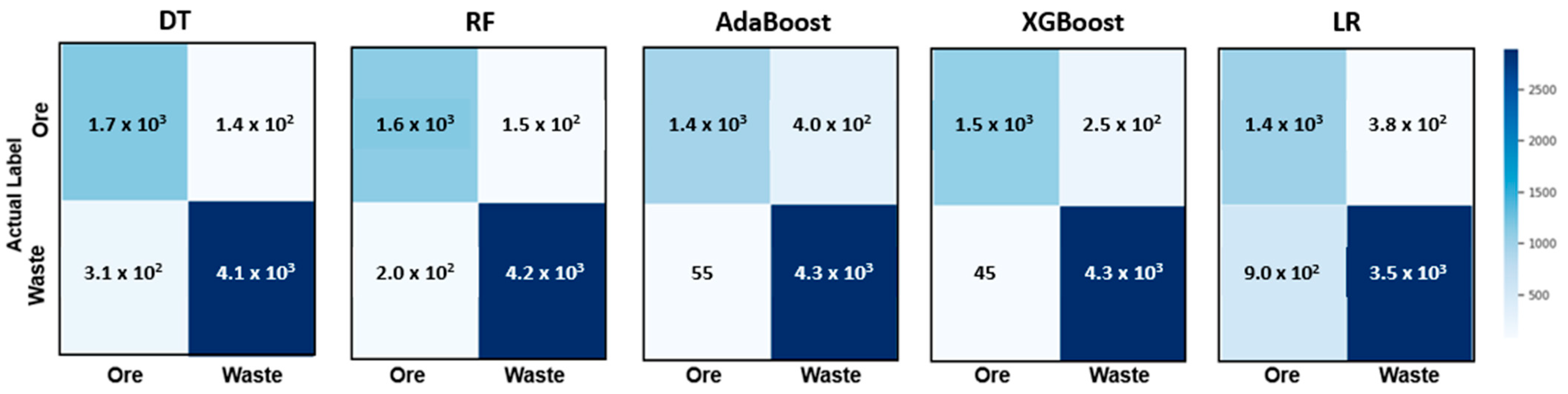
Figure 4 presents the predictions through the confusion matrix for each model for the scenario that contains all input variables (C1). The matrix shows the distribution of the inputs in terms of their original classes and their predicted classes. The matrix is a good tool for visualizing the performance of the classification algorithm in terms of accuracy. The results show that the XGBoost algorithm presented the best performance by assigning the correct predictions (true positive and true negative) for 96% of the estimated base.

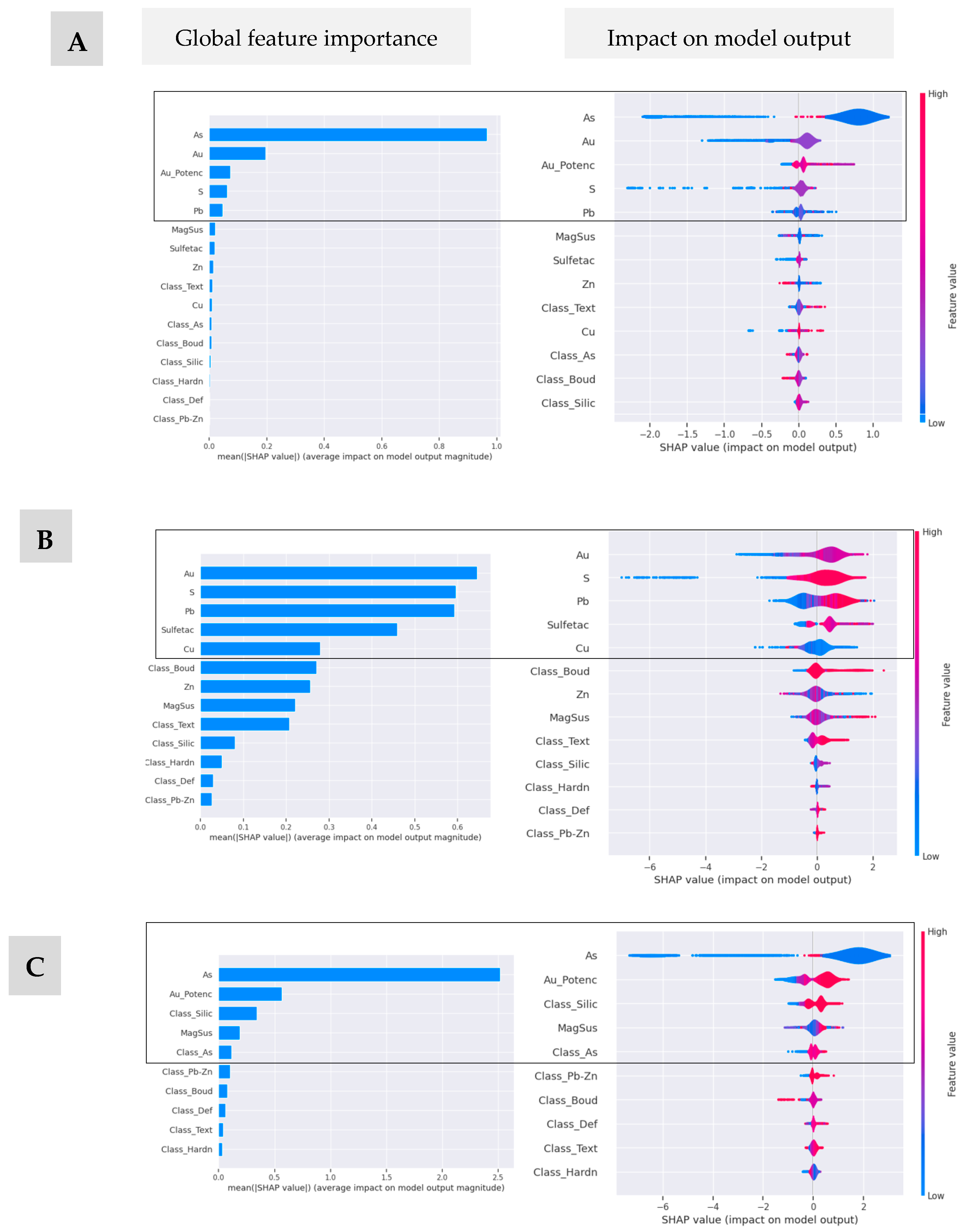
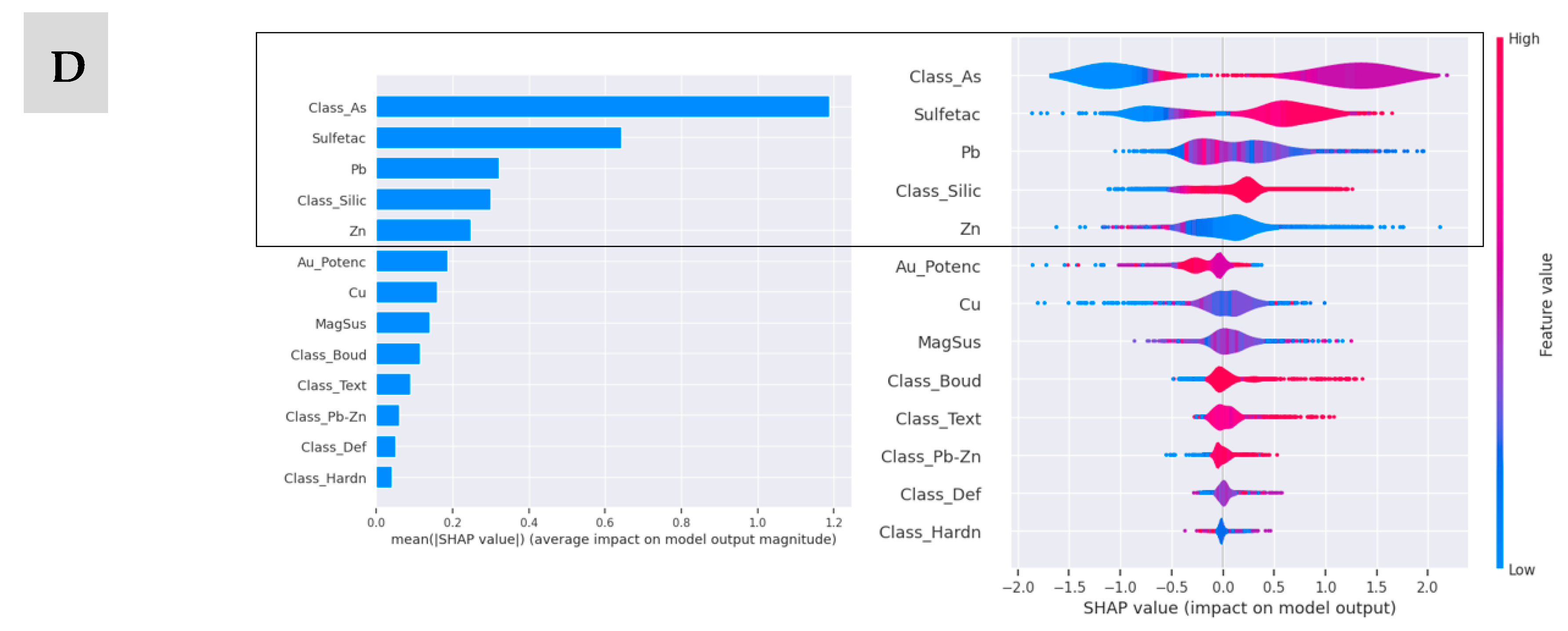
One of the SHAP aspects is the understanding of how a considerable number of numerical and categorical variables (samples) can additively provide explanations for the classified models, since the global and local analysis of the importance of resources can provide insights into the prediction of mineralized levels.

The SHAP values were used to highlight important features and their impact on the classification, which, in a way, can assist in a more detailed analysis of the variable. The results indicate that the variable As was prominent in the predictions, mainly in scenarios C1 and C3. The arsenic class (Class_As), present mainly in scenario C4, had a significant positive weight in the classification. Regarding the impact on the output model, for scenarios C1 and C3, the variable As has a moderate impact in relation to the other input variables. In scenario C2, the variable Au together with S and Pb had a moderate to high positive impact on the prediction of the output model. Finally, in scenario C4, there is a distribution in the impact weights under the classification model among the variables Class_As, Sulfetac, Pb, Class_Silic, and Zn. Important contributions are observed for sulfidation (Sulfetac), potential for gold occurrence in a favorable formation context, such as predominance of boudinage, deformation, and sulfidation. Figure 5 shows the average impact on model output magnitude and impact on model output for the XGBoost algorithm, which presented the best performance.

In general, some relationships of importance between the variables, the weights in the contribution of the predictions between them are difficult to be perceived by decision makers but are explored and analyzed through these implementations.

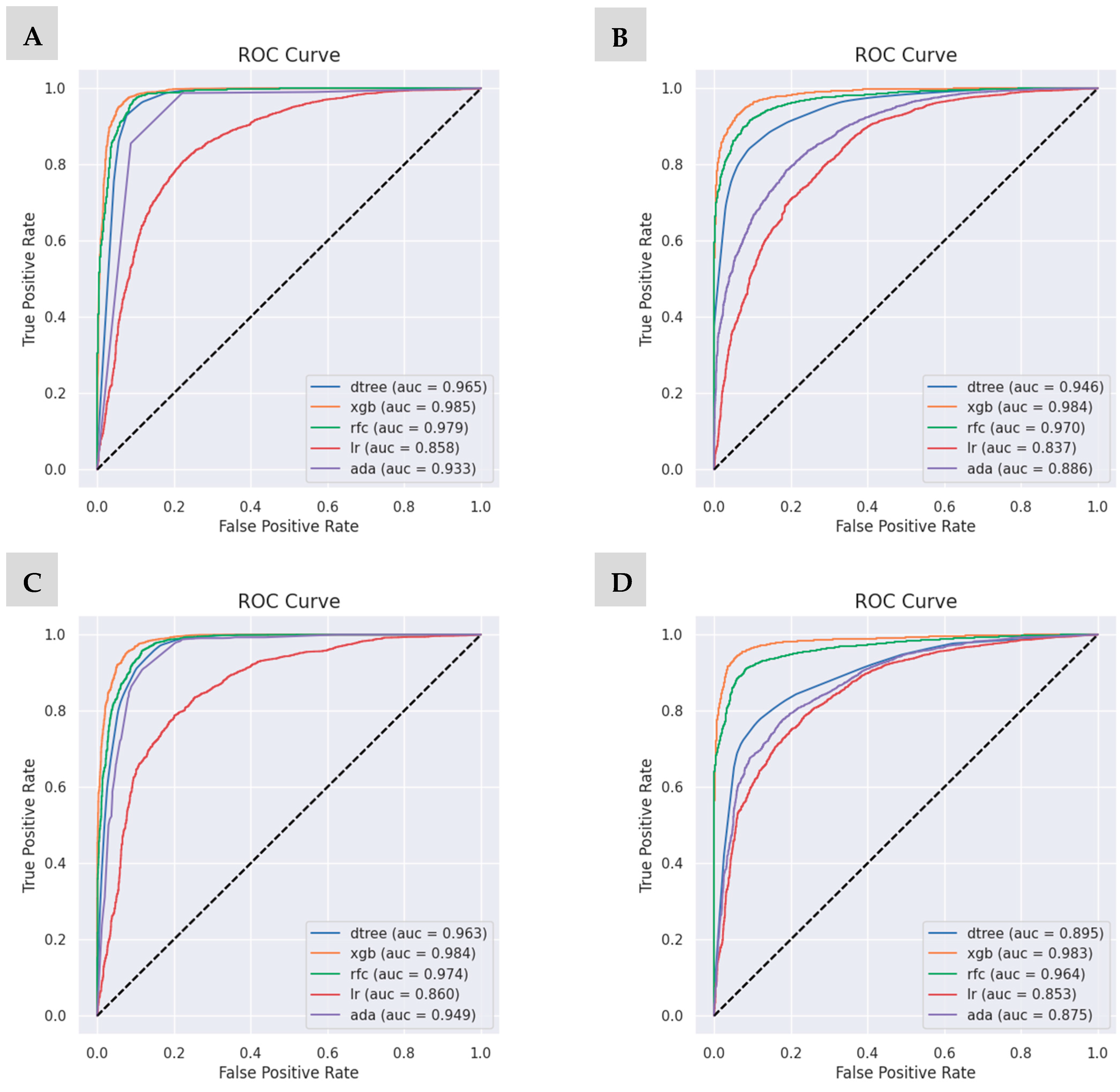
The AUC and ROC curves are used to evaluate the model classification performance of the tested algorithms and are shown in Figure 6. AUC measures the ability of a binary classifier to distinguish classes and is used as a summary of the ROC curve. In addition, it also measures the quality of the model’s predictions, regardless of the classification threshold.

The results show that the XGBoost approach, scenario C1, obtained the highest AUC of 0.985, indicating that the algorithm performs best in the ore/gangue classification for the set of samples studied but with little variation in the other scenarios tested, as well as RF. The LR algorithm together with AdaBoost had the worst performance, also varying across the scenarios. Scenario C2 showed low performance due to the absence of the lowest weight on the arsenic variable in the prediction

5. Discussion

A total of 16,826 instances were used in the study, with 6730 tested (40% of the dataset). Seventeen input variables were considered, combining numerical (grades) and categorical data (textural and mineralogical descriptions). A key challenge was the subjectivity in categorical descriptions, such as texture and mineral predominance. Five supervised ML algorithms were evaluated across four scenarios (Table 3), using both numerical and categorical inputs. Scenario C1, which included all variables, achieved the best classification scores. Scenarios C2 and C4 excluded arsenic-related variables (As and Class_As) to assess their impact. Accuracy dropped to 0.93 (C2) and 0.94 (C4), confirming arsenic plays a significant predictive role. Scenario C3 tested the exclusion of Au, S, Pb, Zn, and Cu, further supporting the influence of arsenic. SHAP analysis confirmed As, Au, Sulfetac, Au_Potenc, and Class_As as the most impactful variables, aligning with correlation analysis (e.g., Au-As r = 0.47; S-As r = 0.51; Au-S r = 0.43).

Among the algorithms, XGBoost outperformed others, achieving up to 0.96 accuracy in scenario C1. Its strength lies in handling complex interactions, especially those involving arsenic and gold. In scenario C4, where major chemical elements were excluded, categorical features like Class_As, sulfidation, and Class_Silic played a key role.

Tree-based models (DT, RF, XGBoost, and AdaBoost) demonstrated superior performance due to their boosting mechanisms and tree-splitting strategies. This finding aligns with [66], which showed that RF had the best predictive performance in a similar mineralogical dataset. According to [38], gold is primarily associated with arsenopyrite and pyrite, with secondary associations involving silicates, carbonates, and other sulfides. Increased As and S levels correlate with higher gold content due to sulfide presence. This is evident in the correlation matrix (Figure 3) and SHAP analyses. Furthermore, the presence of secondary minerals like galena and sphalerite (Class_Pb-Zn) also contributes locally to gold prediction.

The deposit under study is a relevant example that corroborates the modeling approach. This world-class orogenic gold deposit is characterized by low-grade, large-scale mineralization where gold is closely associated with arsenopyrite and pyrite within meta-sedimentary rocks. In this context, arsenic acts as a reliable geometallurgical indicator, confirming the importance of As-related variables observed in the SHAP analysis. Furthermore, the textural features, such as sulfidation degree and rock hardness, play a critical role in gold recovery, especially due to the fine and disseminated nature of the mineralization. These factors reinforce the predictive relevance of categorical variables, even in scenarios where Au content is excluded from the model.

Lastly, high gold grades do not always indicate viable mineralization due to factors such as hardness and low sulfidation, which affect recovery in grinding and flotation processes. Thus, arsenic and gold remain central to mineralization control, as confirmed across all scenarios.

6. Conclusions

Four supervised algorithms that use decision trees as a basis were tested to solve classification problems. Only one model was tested (LR) based on the binomial distribution. In general, the use of classification algorithms is a simple and effective approach to build a classification structure that can predict values from complex input data. The XGBoost model, based on decision trees, obtained the best result with an accuracy of 0.96 in scenario C1, 0.93 for C2, 0.95 for scenario C3, and 0.94 for scenario C4. The other three models, DT, RF, and AdaBoost obtained better performances compared with LR. To evaluate and validate the results, the performance curves metric MSE, precision, recall, and ROC-AUC were used. The differentiation between the scenarios was considered, as well as the distribution of numerical variables, represented by the different sample contents, and the categorical variables, represented by the frequency distributions of the intrinsic characteristics for each variable. There were no significant differences when observing the ROC-AUC results for the XGBoost and RF decision tree-based algorithms for the scenarios evaluated. However, the XGBoost algorithm presented values above 0.98 in all scenarios. The LR algorithm consistently presented lower scores, with values below 0.85 in all scenarios, representing the worst performance.

The multivariate relationships indicate a moderate correlation between the mineralized level (ore) with sulfidation, Class_As, and the content of As, S, and Au, not indicating a strong relationship with other variables. This characteristic of the mineralized levels in relation to the occurrence of S minerals, sulfidation, and frequency of As is related to the type of ore defined in the beneficiation processes, which can be classified as free-milling or refractory. Free-milling gold ores are defined as those in which more than 90% of the gold can be recovered by leaching via conventional cyanidation. Refractory ores present low gold recovery or acceptable recovery with the significant use of reagents or more complex treatment processes.

In conclusion, the results highlight the importance of applying explainable machine learning models to predict mineral levels based on numerical variables, represented by grades, and categorical variables, by frequency classes obtained by description of drillholes. The local and global impact variables, obtained by SHAP analysis, proved to be a useful tool to improve the performance of operations, supporting decision makers due to their local and global predictive capacity. In fact, the numerical variables, represented by grades, have greater weight in the application of the algorithms, but they can be used with the categorical variables to provide more robustness in the final prediction. The classification result in scenario C1 shows the complement between the numerical and categorical variables in the analyses. The XGBoost classifier outperformed other algorithms, showing great possibility of implementation in analysis routines.

References

1. Chryssoulis, S.L.; Mcmullen, J. Mineralogical investigation of gold ores. In Advances in Gold Ore Processing, Developments in Mineral Processing; Adams, M.D., Wills, B.A., Eds.; Elsevier: Amsterdam, The Netherlands, 2005; Volume 15, pp. 21–71. [Google Scholar]
2. Schach, E.; Buchmann, M.; Tolosana-Delgado, R.; Leißner, T.; Kern, M.; Van Den Boogaart, G.; Rudolph, M.; Peuker, U.A. Multidimensional characterization of separation processes—Part 1: Introducing kernel methods and entropy in the context of mineral processing using SEM-based image analysis. Miner. Eng. 2019, 137, 78–86. [Google Scholar] [CrossRef]
3. Shouwastra, R.P.; Smith, A.J. Devepments in mineralogical techniques—What about mineralogists? Miner. Eng. 2011, 24, 1224–1228. [Google Scholar] [CrossRef]
4. Chryssoulis, S.L.; Mcintyre, N.S.; Mycroft, J.R. Determination of gold in natural sulphide minerals using X-ray photoelectron spectroscopy. Can. Mineral. 1993, 31, 231–240. [Google Scholar]
5. Marsden, J.; House, I. The Chemistry of Gold Extraction; Ellis Horwood: London, UK, 1992. [Google Scholar]
6. Fisher, L.; Gazley, M.F.; Baensch, A.; Barnes, S.J.; Cleverley, J.; Duclaux, G. Resolution of Geochemical and Lithostratigraphic Complexity: A Workflow for Application of Portable X-Ray Fluorescence to Mineral Exploration. Geochem. Explor. Environ. Anal. 2014, 14, 149–159. [Google Scholar] [CrossRef]
7. Gazley, M.F.; Tutt, C.M.; Fisher, L.A.; Latham, A.R.; Duclaux, G.; Taylor, M.D.; de Beer, S.L. Objective geological logging using portable XRF geochemical multi-element data at Plutonic Gold Mine, Marymia Inlier, Western Australia. J. Geochem. Explor. 2014, 143, 74–83. [Google Scholar] [CrossRef]
8. Becker, M.; Jardine, M.A.; Miller, J.A.; Harris, M. X-Ray Computed Tomography: A Geometallurgical Tool for 3D Textural Analysis of Drill Core? In Proceedings of the 3rd AusIMM International Geometallurgy Conference, Perth, Australia, 15–17 June 2016; pp. 231–240. [Google Scholar]
9. Bonnici, N.K. The Mineralogical and Textural Characteristics of Copper-Gold Deposits Related to Mineral Processing Attributes. Ph.D. Thesis, University of Tasmania, Hobart, Tasmania, 2012; p. 498. [Google Scholar]
10. Nguyen, A.J.; Nguyen, J.K.; Manlapig, E. A New Semi-Automated Method to Rapidly Evaluate the Processing Variability of the Ore Body. In Proceedings of the Third AusIMM International Geometallurgy Conference, Perth, Australia, 15–17 June 2016; pp. 145–151. [Google Scholar]
11. Cracknell, M.; Parbhakar-Fox, A.; Jackson, L.; Savinova, E. Automated acid rock drainage indexing from drill core imagery. Minerals 2018, 8, 571. [Google Scholar] [CrossRef]
12. Lamberg, P. Particles—The bridge beteween geology and metallurgy. In Proceedings of the Conference in Mineral Engineering, Lulea, Sweden, 8–9 February 2011; pp. 1–16. [Google Scholar]
13. Ersoy, A.; Waller, M.D. Textural characterization of rocks. Eng. Geol. 1995, 39, 123–136. [Google Scholar] [CrossRef]
14. Ikotun, A.M.; Ezugwu, A.E.; Abualigah, L.; Abuhaija, B.; Heming, J. K-means clustering algorithms: A comprehensive review, variants analysis, and advances in the era of big data. Inf. Sci. 2023, 622, 178–210. [Google Scholar] [CrossRef]
15. Deutsch, C.V.; Lan, Z. The beta distribution for categorical variables at different support. In Progress in Geomathematics; Springer: Berlin/Heidelberg, Germany, 2008; pp. 445–456. [Google Scholar]
16. Rossi, M.E.; Deutsch, C.V. Mineral Resource Estimation; Springer Science & Business Media: Berlin/Heidelberg, Germany, 2013; p. 332. [Google Scholar] [CrossRef]
17. Chaube, S.; Goverapet Srinivasan, S.; Rai, B. Applied machine learning for predicting the lanthanide-ligand binding affinities. Sci. Rep. 2020, 10, 14322. [Google Scholar] [CrossRef]
18. Jain, D.; Chaube, S.; Khullar, P.; Srinivasan, S.G.; Rai, B. Bulk and surface DFT investigations of inorganic halide perovskites screened using machine learning and materials property databases. Phys. Chem. Chem. Phys. 2019, 21, 19423–19436. [Google Scholar] [CrossRef]
19. Kaushik, J.; Dodagoudar, G.R. Explainable machine learning model for liquefaction potential assessment of soils using XGBoost-SHAP. Soil Dyn. Earthq. Eng. 2023, 165, 1–22. [Google Scholar] [CrossRef]
20. Zheng, L.; Wang, C.; Chen, X.; Song, Y.; Meng, Z.; Zhang, R. Evolutionary machine learning builds smart education big data platform: Data-driven higher education. Appl. Soft Comput. 2023, 136, 1–10. [Google Scholar] [CrossRef]
21. Haykin, S. Redes neurais artificiais. In Princípios e Pratica; Bookman: Porto Alegre, Brazil, 2001. [Google Scholar]
22. Kohonen, T. Self-Organizing Maps, 2nd ed.; Springer: Berlin, Germany, 1997. [Google Scholar]
23. Fraser, S.J.; Dickson, B.L. A new method for data integration and integrated data interpretation: Self-organizing maps. In Proceedings of the 5th Decennial International Conference on Mineral Exploration, Toronto, ON, Canada, 9–12 September 2007; Expanded Abstracts. pp. 907–910. [Google Scholar]
24. Taha, K. Semi-supervised and un-supervised clustering: A review and experimental evaluation. Inf. Syst. 2023, 114, 1–34. [Google Scholar] [CrossRef]
25. Kaelbling, L.P.; Littman, M.L.; Moore, A.W. Reinforcement learning: A survey. J. Artif. Intell. Res. 1996, 4, 237–285. [Google Scholar] [CrossRef]
26. Carrasco, P.; Chilès, J.P.; Séguret, S.A. Additivity, metallurgical recovery, and grade. In Proceedings of the 8th International Geostatistics Congress, Santiago, Chile, 1–5 December 2008. [Google Scholar]
27. Coward, S.; Vann, J.; Dunham, S.; Stewart, M. The primary-response framework for geometallurgical variables. In Proceedings of the Seventh International Mining Geology Conference, Perth, Australia, 17–19 August 2009; pp. 109–113. [Google Scholar]
28. Keeney, L. The Development of a Novel Method for Integrating Geometallurgical Mapping and Orebody Modelling. Ph.D. Thesis, The University of Queensland, Brisbane, Australia, 2010. [Google Scholar]
29. Keeney, L.; Walters, S.G. A methodology for geometallurgical mapping and orebody modelling. In Proceedings of the 1st AusIMM International Geometallurgy Conference, Brisbane, Australia, 5–7 September 2011; pp. 217–225. [Google Scholar]
30. Deutsch, J.L.; Palmer, K.; Deutsch, C.V.; Szymanski, J.; Etsell, T.H. Spatial modeling of geometallurgical properties: Techniques and a case study. Nat. Resour. Res. 2016, 25, 161–181. [Google Scholar] [CrossRef]
31. Sepúlveda, E.; Dowd, P.A.; Xu, C. Fuzzy clustering with spatial correction and its application to geometallurgical domaining. Math. Geosci. 2018, 50, 895–928. [Google Scholar] [CrossRef]
32. Bhuiyan, M.; Esmaieli, K.; Ordóñez-Calderón, J.C. Application of data analytics techniques to establish geometallurgical relationships to Bond work index at the Paracutu Mine, Minas Gerais Brazil. Minerals 2019, 9, 295–302. [Google Scholar] [CrossRef]
33. Rajabinasab, B.; Asghari, O. Geometallurgical domaining by cluster analysis: Iron ore deposit case study. Nat. Resour. Res. 2019, 28, 665–684. [Google Scholar] [CrossRef]
34. Rincon, J.; Gaydardzhiev, S.; Stamenov, L. Coupling comminution indices and mineralogical features as an approach to a geometallurgical characterization of a copper ore. Miner. Eng. 2019, 130, 57–66. [Google Scholar] [CrossRef]
35. Koch, P.H.; Lund, C.; Rosenkranz, J. Automated drill core mineralogical characterization method for texture classification and modal mineralogy estimation for geometallurgy. Min. Eng. 2019, 136, 99–109. [Google Scholar] [CrossRef]
36. Russell, S.J.; Norvig, P. Artificial Intelligence: A Modern Approach, 4th ed.; Pearson: Upper Saddle River, NJ, USA, 2020; p. 1136. [Google Scholar]
37. McCoy, J.T.; Auret, L. Machine learning applications in minerals processing: A review. Min. Eng. 2019, 132, 95–109. [Google Scholar] [CrossRef]
38. Costa, F.R.; Nery, G.P.; Carneiro, C.C.; Kahn, H.; Ulsen, C. Mineral characterization of low grade ore to support geometallurgy. J. Mater. Res. Technol. 2022, 21, 2841–2852. [Google Scholar] [CrossRef]
39. Costa, F.R.; Carneiro, C.C.; Ulsen, C. Imputation of gold recovery data from low grade gold ore using artificial neural network. Minerals 2023, 13, 340. [Google Scholar] [CrossRef]
40. Lishchuk, V.; Lund, C.; Ghorbani, Y. Evaluation and comparison of different machine learning methods to integrate sparse process data into a spatial model in geometallurgy. Min. Eng. 2019, 134, 156–165. [Google Scholar] [CrossRef]
41. Shapley, L.S. A value for n -person games. In The Shapley Value: Essays in Honor of Lloyd S. Shapley; Roth, A.E., Ed.; Cambridge University Press: Cambridge, UK, 1988; pp. 31–40. [Google Scholar] [CrossRef]
42. Lehmann, E.L.; George, C. Theory of Point Estimation, 2nd ed.; Springer: New York, NY, USA, 1998. [Google Scholar]
43. Ting, K.M. Confusion matrix. In Encyclopedia of Machine Learning; Sammut, C., Webb, G.I., Eds.; Springer US: Boston, MA, USA, 2010; p. 209. [Google Scholar] [CrossRef]
44. Navin, M.; Pankaja, R. Performance analysis of text classification algorithms using confusion matrix. Int. J. Eng. Tech. Res. 2016, 4, 75–78. [Google Scholar]
45. Sammut, C.; Webb, G.I. Encyclopedia of Machine Learning and Data Mining; Springer: New York, NY, USA, 2017. [Google Scholar]
46. Maimon, O.; Rokach, L. Ensemble of decision trees for mining manufacturing data sets. In:Soft Computing for Knowledge Discovery and Data Mining; Springer: Boston, MA, USA, 2008; pp. 195–217. [Google Scholar] [CrossRef]
47. Sáez, J.A.; Galar, M.; Luengo, J.; Herrera, F. Tackling the problem of classification with noisy data using multiple classifier systems: Analysis of the performance and robustness. Inf. Sci. 2013, 247, 1–20. [Google Scholar] [CrossRef]
48. Priyam, A.; Gupta, R.; Rathee, A.; Srivastava, S. Comparative analysis of decision tree classification algorithms. Int. J. Curr. Eng. Technol. 2013, 3, 334–337. [Google Scholar]
49. Breiman, L. Random forests. Mach Learn 2001, 45, 5–32. [Google Scholar] [CrossRef]
50. Shah, K.; Patel, H.; Sanghvi, D.; Shah, M. A comparative analysis of logistic regression, random forest and KNN models for the text classification. Augment. Hum. Res. 2020, 5, 1–16. [Google Scholar] [CrossRef]
51. Raschka, S.; Mirjalili, V. Python Machine Learning, 3rd ed.; Packt Publishing Ltd.: Birmingham, UK, 2019. [Google Scholar]
52. Freund, Y.; Schapire, R.E. A desicion-theoretic generalization of on-line learning and an application to boosting. In Computational Learning Theory; Vitanyi, P., Ed.; Springer: Berlin/Heidelberg, Germany, 1995; pp. 23–37. [Google Scholar]
53. Chen, T.; Guestrin, C. XGBoost: A Scalable Tree Boosting System. In Proceedings of the 22nd ACM SIGKDD International Conference on Knowledge Discovery and Data Mining, San Francisco, CA, USA, 13–17 August 2016; pp. 785–794. [Google Scholar] [CrossRef]
54. Friedman, J.H. Greedy function approximation: A gradient boosting machine. Ann. Stat. 2001, 29, 1189–1232. [Google Scholar] [CrossRef]
55. Bisong, E. Logistic Regression. In Building Machine Learning and Deep Learning Models on Google Cloud Platform; Apress: Berkeley, CA, USA, 2019; pp. 243–250. [Google Scholar] [CrossRef]
56. Lundberg, S.; Lee, S.I. An Unexpected Unity Among Methods for Interpreting Model Predictions. In Proceedings of the 29th Conference on Neural Information Processing Systems (NeurIPS 2016), Barcelona, Spain, 5–10 December 2016; Lee, D.D., Sugiyama, M., Luxburg, U.V., Guyon, I., Garnett, R., Eds.; Curran Associates, Inc.: Red Hook, NY, USA, 2016; pp. 1–6. [Google Scholar] [CrossRef]
57. Lundberg, S.M.; Lee, S.I. A unified approach to interpreting model predictions. In Proceedings of the 31st Conference on Neural Information Processing Systems (NIPS), Long Beach, CA, USA, 4–9 December 2017; Guyon, I., Luxburg, U.V., Bengio, S., Wallach, H., Fergus, R., Vishwanathan, S., Garnett, R., Eds.; Curran Associates, Inc.: Long Beach, CA, USA, 2017; pp. 4768–4777. [Google Scholar] [CrossRef]
58. Liu, X.; Aldrich, C. Explaining anomalies in coal proximity and coal processing data with Shapley and tree-based models. Fuel 2023, 335, 126891. [Google Scholar] [CrossRef]
59. Lundberg, S.M.; Erion, G.G.; Lee, S.I. Consistent Individualized Feature Attribution for Tree Ensembles. arXiv 2018, arXiv:1802.03888. [Google Scholar] [CrossRef]
60. Lundberg, S.M.; Erion, G.G.; Chen, H.; DeGrave, A.; Prutkin, J.M.; Nair, B.; Katz, R.; Himmelfarb, J.; Bansal, N.; Lee, S.I. From local explanations to global understanding with explainable AI for trees. Nat. Mach. Intell. 2020, 2, 56–67. [Google Scholar] [CrossRef] [PubMed]
61. Van der Walt, S.; Colbert, S.C.; Varoquaux, G. The NumPy Array: A Structure for Efficient Numerical Computation. Comput. Sci. Eng. 2011, 13, 22–30. [Google Scholar] [CrossRef]
62. Mckinney, W. Pandas: A Foundational Python Library for Data Analysis and Statistics. Python High Perform. Sci. Comput. 2011, 14, 1–9. [Google Scholar]
63. Pedregosa, F.; Varoquaux, G.; Gramfort, A.; Michel, V.; Thirion, B. Scikit-learn: Machine Learning in Python. J. Mach. Learn. Res. 2011, 12, 2825–2830. [Google Scholar]
64. Hunter, J.D. Matplotlib: A 2D Graphics Environment. Comput. Sci. Eng. 2007, 9, 90–95. [Google Scholar] [CrossRef]
65. Costa, F.R.; Carneiro, C.C.; Ulsen, C. Self-Organizing Maps Analysis of Chemical–Mineralogical Gold Ore Characterization in Support of Geometallurgy. Mining 2023, 3, 230–240. [Google Scholar] [CrossRef]
66. Costa, F.R.; Carneiro, C.C.; Ulsen, C. Predicting gold accessibility from mineralogical characterization using machine learning algorithms. J. Mater. Res. Technol. 2024, 29, 668–677. [Google Scholar] [CrossRef]
Figure 1. Definition of the confusion matrix. The matrix is organized into real data and predicted data, categorized by rows and columns and combining true positive (TP) data, false positive (FP) data, false negative (FN) data, and true negative (TN) data.
Geosciences 15 00248 g001
Figure 2. Flowchart of activities performed until ore classification.
Geosciences 15 00248 g002
Figure 3. Correlation matrix of numerical and categorical variables.
Geosciences 15 00248 g003
Figure 4. Confusion matrix for Scenario C1 showing the distribution of predicted vs. actual classes for each ML algorithm.
Geosciences 15 00248 g004
Figure 5. Importance of the features for the XGBoost model implemented to predict ore, considering different scenarios by SHAP values. (A) scenario C1; (B) scenario C2; (C) scenario C3; and (D) scenario C4.
Geosciences 15 00248 g005aGeosciences 15 00248 g005b
Figure 6. Comparison of the ROC curves between different models in the four-scenario dataset. (A) scenario C1; (B) scenario C2; (C) scenario C3; and (D) scenario C4.
Geosciences 15 00248 g006