Topographic Control of Wind- and Thermally Induced Circulation in an Enclosed Water Body

Abstract

The dynamics of large lake circulations are strongly modulated by wind forcing, thermal gradients, and shoreline topography, yet their integrated effects remain insufficiently quantified. To address this, numerical simulations were conducted in Lake Biwa to clarify the mechanisms underlying wind- and thermally driven gyres, with a focus on the influence of bathymetric asymmetry. In wind-driven cases, zonal and meridional wind stress gradients were imposed, revealing that cyclonic wind shear generated strong surface vorticity (up to 2.0 × 10⁻⁶ s⁻¹) in regions with gently sloped shores, while steep slopes suppressed anticyclonic responses. Cyclonic forcing induced upwelling in the lake center, with baroclinic return flows stabilizing the vertical circulation structure. In windless thermal experiments, surface temperature gradients of ±2.5 °C were applied to simulate seasonal heating and cooling. Cyclonic circulation predominated in warm seasons due to convergence and heat accumulation along gently sloping shores, whereas winter cooling produced divergent flows and anticyclonic gyres. The southern and eastern lake margins, characterized by mild slopes, consistently enhanced convergence and vertical mixing, while steep western and northern slopes limited circulation intensity. These results demonstrate that shoreline slope asymmetry plays a decisive role in regulating both wind- and thermally induced circulations, offering insights into physical controls on transport and stratification in enclosed lake systems.

1. Introduction

In large stratified lakes and semi-enclosed seas, basin-scale horizontal circulations resembling oceanic gyres are widely recognized as emergent features shaped by the interplay between external forcings—such as wind stress, surface heat fluxes, and the Coriolis effect—and internal controls, including vertical stratification and complex bottom topography. These gyre-like flows are not merely passive responses to external drivers; rather, they actively regulate the basin’s physical and ecological dynamics by modulating horizontal transport, vertical mixing, nutrient distribution, oxygenation processes, and primary production across spatial and temporal scales [1].

In the North American Great Lakes, particularly in Lakes Michigan, Huron, and Ontario, persistent cyclonic gyres have been observed during the spring stratification period. These gyres are often initiated by wind-driven geostrophic adjustment after the establishment of a thermal bar that suppresses vertical mixing. Lagrangian drifter studies and remote sensing have consistently documented these circulations, revealing spatial extents of tens to hundreds of kilometers and lifetimes ranging from weeks to months [2,3,4].

Similarly, in large European lakes such as Lake Geneva, numerical modeling has demonstrated the importance of Rossby waves, density fronts, and slope-driven flows induced by shoreline geometry in the emergence of large-scale gyres [5]. In semi-enclosed marginal seas like the Baltic and Black Seas, Earth’s rotation and salinity stratification foster quasi-steady mesoscale eddies, coastal jets, and internal wave activity. These features exert a profound influence on long-range material transport and vertical oxygen exchange, particularly in hypoxic bottom layers [6,7].

In Japan, Lake Biwa—the country’s largest freshwater lake—exhibits robust gyre structures, especially within its deep northern basin, where thermal stratification develops during the warm season. Observational data from moored buoys, acoustic Doppler current profilers (ADCPs), and satellite-derived surface temperature imagery have repeatedly identified the formation of clockwise gyres from spring through autumn [8]. These gyres tend to be concentrated in the central northern basin and are associated with sloping isopycnals, indicating a quasi-geostrophic balance [9].

Two primary physical mechanisms have been proposed to explain the formation of these gyres in Lake Biwa. First, wind-driven circulation, where prevailing northwesterly winds induce surface Ekman transport toward the lake center, creates horizontal pressure gradients that establish a geostrophic return flow—a dynamic analogous to Sverdrup circulation in the ocean [10]. Second, thermally driven circulation, wherein diurnal heating and nocturnal cooling along the nearshore zones generate lateral temperature gradients that drive buoyancy-induced, cross-shore convection cells, contributing to horizontal recirculation [11].

Previous studies have attempted to quantify the role of wind stress, thermal forcing, shoreline geometry, and stratification intensity using field data and idealized simulations [12,13,14,15]. However, the extent to which these forcing mechanisms interact nonlinearly under realistic meteorological and bathymetric conditions to initiate, maintain, and regulate gyre structures remains insufficiently understood.

The aim of this study is to elucidate the dynamical mechanisms underlying the formation and maintenance of gyres in Lake Biwa by conducting three-dimensional hydrodynamic simulations based on realistic topographic and meteorological inputs [16]. Sensitivity experiments were performed to isolate the effects of wind and thermal forcing, and their respective contributions to gyre development were evaluated.

2. Methodology

2.1. Numerical Simulation

In this study, the fundamental equations of the three-dimensional flow field model [16] are formulated based on the Boussinesq approximation and the hydrostatic assumption in the vertical direction. The governing equations consist of the momentum equations, the continuity equation, and the advection–diffusion equation for temperature and are given as follows:

$$\begin{array}{c}{\displaystyle \frac{\partial u}{\partial t}}+u{\displaystyle \frac{\partial u}{\partial x}}+v{\displaystyle \frac{\partial u}{\partial y}}+w{\displaystyle \frac{\partial u}{\partial z}}-fv=-{\displaystyle \frac{1}{{\rho }_0}}{\displaystyle \frac{\partial p}{\partial x}}+A_h{\displaystyle \frac{{\partial }^{2}u}{\partial x^2}}+A_h{\displaystyle \frac{{\partial }^{2}u}{\partial y^2}}+A_z{\displaystyle \frac{{\partial }^{2}u}{\partial z^2}}-{\displaystyle \frac{g}{\rho }}{\int }_z^0{\displaystyle \frac{\partial \rho }{\partial x}}dz\end{array}$$

(1)

$$\begin{array}{c}{\displaystyle \frac{\partial v}{\partial t}}+u{\displaystyle \frac{\partial v}{\partial x}}+v{\displaystyle \frac{\partial v}{\partial y}}+w{\displaystyle \frac{\partial v}{\partial z}}+fu=-{\displaystyle \frac{1}{{\rho }_0}}{\displaystyle \frac{\partial p}{\partial y}}+A_h{\displaystyle \frac{{\partial }^{2}v}{\partial x^2}}+A_h{\displaystyle \frac{{\partial }^{2}v}{\partial y^2}}+A_z{\displaystyle \frac{{\partial }^{2}v}{\partial z^2}}-{\displaystyle \frac{g}{\rho }}{\int }_z^0{\displaystyle \frac{\partial \rho }{\partial y}}dz\end{array}$$

(2)

$$0=-{\displaystyle \frac{1}{{\rho }_0}}{\displaystyle \frac{\partial p}{\partial z}}-{\displaystyle \frac{\rho }{{\rho }_0}}g$$

(3)

$${\displaystyle \frac{\partial u}{\partial x}}+{\displaystyle \frac{\partial v}{\partial y}}+{\displaystyle \frac{\partial w}{\partial z}}=0$$

(4)

$$\begin{array}{c}{\displaystyle \frac{\partial T}{\partial t}}+u{\displaystyle \frac{\partial T}{\partial x}}+v{\displaystyle \frac{\partial T}{\partial y}}+w{\displaystyle \frac{\partial T}{\partial z}}=K_h{\displaystyle \frac{{\partial }^{2}T}{\partial x^2}}+K_h{\displaystyle \frac{{\partial }^{2}T}{\partial y^2}}+K_z{\displaystyle \frac{{\partial }^{2}T}{\partial z^2}}\end{array}$$

(5)

where u, v, w are the velocities in the x, y, z directions (m/s), respectively; T is the water temperature (K); p is the pressure (N/m²); $\rho$ is the lake density (kg/m³); ${\rho }_0$ is the reference lake density (=103 kg/m³); g is the gravitational acceleration (=9.8 m/s²); f is the Coriolis parameter (=8.37 × 10⁻⁵/s); A_h is the horizontal eddy viscosity (=1.0 m²/s); K_h is the horizontal eddy diffusion coefficient (=1.0 m²/s); A_z is the vertical eddy viscosity (m²/s); and K_z is the vertical eddy diffusion coefficient (m²/s). The terms on the left-hand side of the momentum equations represent the local acceleration and nonlinear advection of momentum and the Coriolis force. The right-hand side includes the pressure gradient force and turbulent momentum diffusion represented by the horizontal (A_h) and vertical (A_v) eddy viscosity coefficients. The last terms in Equations (1) and (2) account for the baroclinic pressure gradient, which arises from horizontal density variations under stratification. The horizontal eddy viscosity and eddy diffusion coefficient values described above have been shown to play a decisive role in the shape of the gyre in Lake Biwa.

The Richardson number, a dimensionless parameter expressing flow stability under stratification, is employed to calculate A_z and K_z. For the vertical eddy viscosity and eddy diffusion coefficient, they are defined as

$$\begin{array}{c}Ri=-{\displaystyle \frac{g}{{\rho }_0}}{\displaystyle \frac{\frac{\partial \rho }{\partial z}}{{\left(\frac{\partial U_w}{\partial z}\right)}^2}}\end{array}$$

(6)

$$\begin{array}{c}{A}_z={\displaystyle \frac{0.0001}{\left(1.0+5.2Ri\right)}}, K_z={\displaystyle \frac{0.0001}{{\left(1.0+\frac{10}{3}\times Ri\right)}^{\frac{3}{2}}}}\end{array}$$

(7)

where $U_w=\sqrt{u^2+v^2}$ is the horizontal velocity (m/s).

In summer, a thermocline typically forms between 10 and 20 m depth in Lake Biwa. Meteorological data for calculating surface heat fluxes and wind-induced surface shear stress were obtained from the Japan Meteorological Agency (JMA) mesoscale numerical forecast analysis. Air temperature, atmospheric pressure, wind direction and speed, and relative humidity over Lake Biwa were derived from the JMA’s Grid Point Value Meso-Scale Model (GPV MSM), which provides data at a spatial resolution of approximately 5 km (0.0625° longitude × 0.05° latitude) and a temporal resolution of one hour. These variables were horizontally interpolated onto each surface mesh of the hydrodynamic model. Hourly solar radiation data were acquired from the Hikone Meteorological Observatory (35°16′30″ N, 136°14′36″ E) and assumed to be spatially uniform over the lake. Figure 1 shows representative air temperature and wind speed from the Hikone Meteorological Observatory.

River inflows were excluded from the simulation to minimize the influence of external forcing. These effects, such as river inflow, precipitation, and evaporation, are discussed in Koue et al. [17]. The numerical simulation was conducted over a one-year period, from 1 April 2007 to 31 March 2008. Although volumetric inflows were omitted, seasonal-scale energy exchanges at the lake surface were explicitly reproduced using heat budget calculations [18]. Shortwave radiation was attenuated exponentially in the water column as a function of turbidity, and longwave radiation was corrected for cloud cover. In addition, sensible and latent heat fluxes were calculated using a bulk formula based on vertical gradients of air temperature and specific humidity, as well as wind speed. These heat fluxes directly influenced vertical stratification and density structure in the lake. Consequently, thermally driven circulation in the lake was appropriately represented under the given boundary conditions.

2.2. Simulation Cases

To isolate and systematically assess the physical responses of Lake Biwa to wind and thermal forcing, simplified pseudo-weather conditions for air temperature and wind speed were applied within a high-resolution three-dimensional hydrodynamic model (Figure 2). The model domain spans the entire lake, with a horizontal extent of 36 km × 65.5 km discretized by a uniform 500 m structured grid [16]. Vertically, the water column is resolved into 86 layers from the surface to a maximum depth of 107.5 m, with a finer layer thickness (0.5 m) near the surface to accurately capture thermal stratification, gradually increasing to 2.5 m at depth. A staggered grid system is used to solve for temperature, density, pressure, and velocity fields. The coordinate system is oriented with the x- and y-axes aligned west–east and south–north, respectively, and the z-axis directed upward.

The model’s spatial resolution exceeds that of the JMA mesoscale atmospheric model (5 km grid), enabling explicit representation of key topographic features such as basin morphology and sub-basin boundaries. While the pseudo-weather forcing does not retain the full statistical properties of real meteorological variability—such as temporal autocorrelation and stochastic fluctuations—it provides a controlled framework for identifying dominant physical mechanisms. By intentionally excluding time-varying meteorological and hydrological disturbances, the simulations allow a clear interpretation of the lake’s intrinsic dynamical responses to wind- and heat-driven processes.

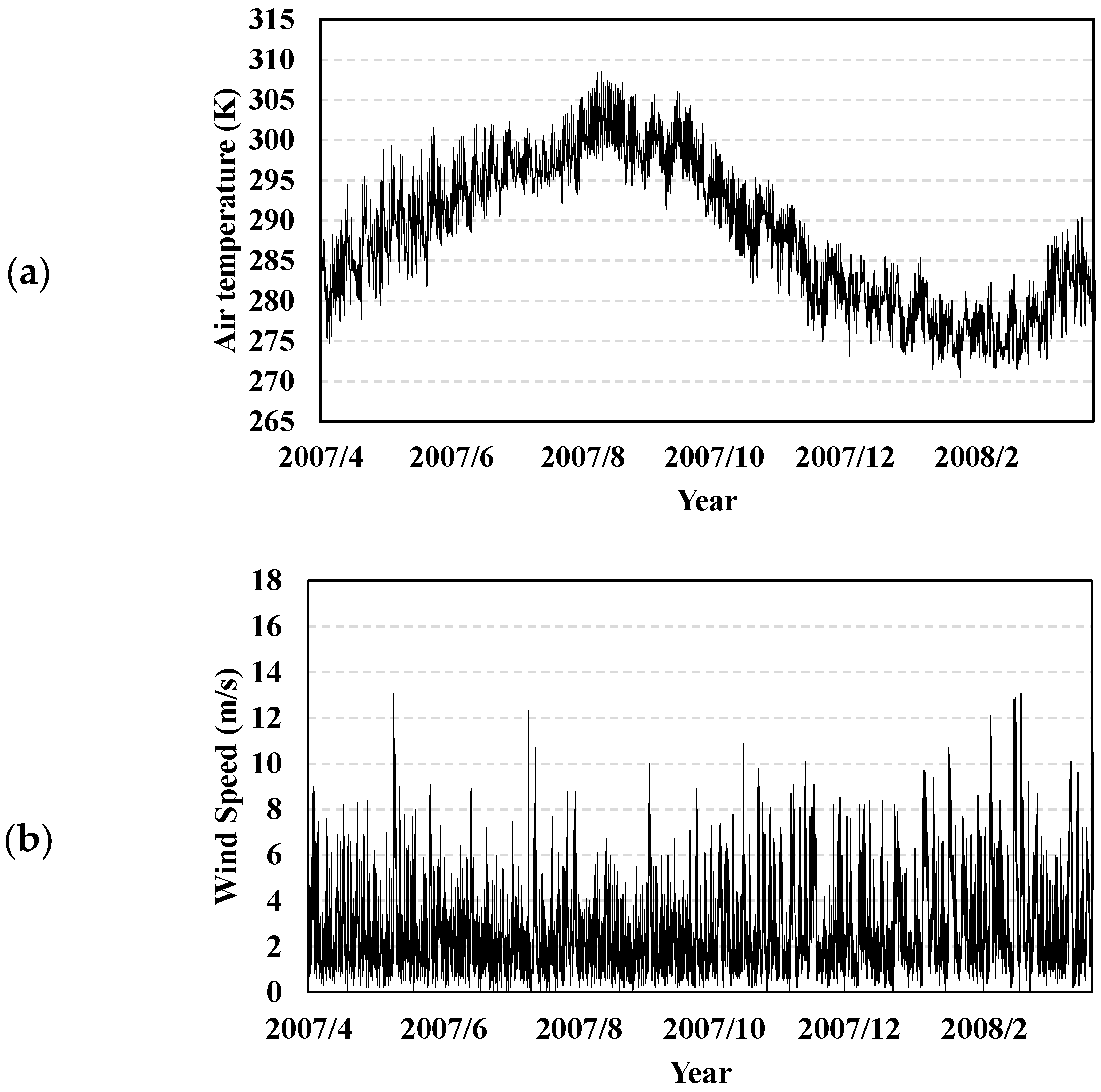
• In the Baseline case, observed values were used for wind speed, wind direction, and air temperature.
• In the WS0_AT25°C case, the wind speed was set to 0 m/s, and the air temperature was fixed at 25 °C; no wind direction was specified.
• In the WSoriginal_AT25°C case, the observed wind speed and wind direction were used, while the air temperature was fixed at 25 °C.
• In the WSeast0towest5m/s_AT25°C and WSeast0towest-5m/s_AT25°C cases, a wind speed gradient from 5 m/s to 0 m/s was imposed from west to east, with the wind direction set to northward and southward, respectively. The air temperature was fixed at 25°C.
• In the WSeast5towest0m/s_AT25°C and WSeast-5towest0m/s_AT25°C cases, a wind speed gradient from 5 m/s to 0 m/s was imposed from east to west, with the wind direction set to northward and southward, respectively. The air temperature was fixed at 25 °C.
• In the WSsouth0tonorth5m/s_AT25°C and WSsouth0tonorth-5m/s_AT25°C cases, a wind speed gradient from 5 m/s to 0 m/s was imposed from north to south, with the wind direction set to eastward and westward, respectively. The air temperature was fixed at 25 °C.
• In the WSsouth5tonorth0m/s_AT25°C and WSsouth-5tonorth0m/s_AT25°C cases, a wind speed gradient from 5 m/s to 0 m/s was imposed from south to north, with the wind direction set to eastward and westward, respectively. The air temperature was fixed at 25 °C.
• In the WS0_AToriginal case, the wind speed was set to 0 m/s, and the observed air temperature was used.
• In the WS0_ATeast+2.5west-2.5°C and WS0_ATeast-2.5west+2.5°C cases, the wind speed was set to 0 m/s, and a horizontal air temperature gradient of +2.5 °C to −2.5 °C and −2.5 °C to +2.5 °C was imposed from east to west, respectively.
• In the WS0_ATsouth+2.5north-2.5°C and WS0_ATsouth-2.5north+2.5°C cases, the wind speed was set to 0 m/s, and a horizontal air temperature gradient of +2.5 °C to −2.5 °C and −2.5 °C to +2.5 °C was imposed from south to north, respectively.

The simulation conditions for each case are summarized in

Table 1. List of simulation cases.

Case	Wind Speed	Wind Direction	Air Temperature
Baseline	Original	Original	Original
WS0_AT25°C	0	-	Constant 25 °C
WSeast0towest5m/s_AT25°C	5 m/s to 0 m/s gradient from west to east	Southerly
WSeast5towest0m/s_AT25°C	5 m/s to 0 m/s gradient from east to west	Southerly
WSsouth0tonorth5m/s_AT25°C	5 m/s to 0 m/s gradient from north to south	Westerly
WSsouth5tonorth0m/s_AT25°C	5 m/s to 0 m/s gradient from south to north	Westerly
WS0_AToriginal	0	-	Original
WS0_ATeast+2.5west-2.5°C			Observed +2.5 °C to −2.5 °C gradient from east to west
WS0_ATeast-2.5west+2.5°C			Observed +2.5 °C to −2.5 °C gradient from west to east
WS0_ATsouth+2.5north-2.5°C			Observed +2.5 °C to −2.5 °C gradient from south to north
WS0_ATsouth-2.5north+2.5°C			Observed +2.5 °C to −2.5 °C gradient from north to south

.

3. Results and Discussion

To quantitatively evaluate the horizontal circulating flow for each simulation case, the vorticity was calculated using the following equation:

$$\begin{array}{c}\omega ={\displaystyle \frac{\partial v}{\partial x}}-{\displaystyle \frac{\partial u}{\partial y}}\end{array}$$

(8)

ω > 0 indicates the counterclockwise gyre, and ω < 0 indicates the clockwise gyre.

For the analysis, average vorticity values are calculated for spring (1 April to 30 June), summer (1 July to 30 September), fall (1 October to 31 December), and winter (1 January to 31 March) and compared for each simulation case. The area where the mean vorticity is calculated is the area where the first gyre, which is a stable flow, is observed (Figure 3). The mean vorticity in the surface layer (0.5–10 m) in the northern part in each season is calculated in the region for a square with a side length of 12 km.

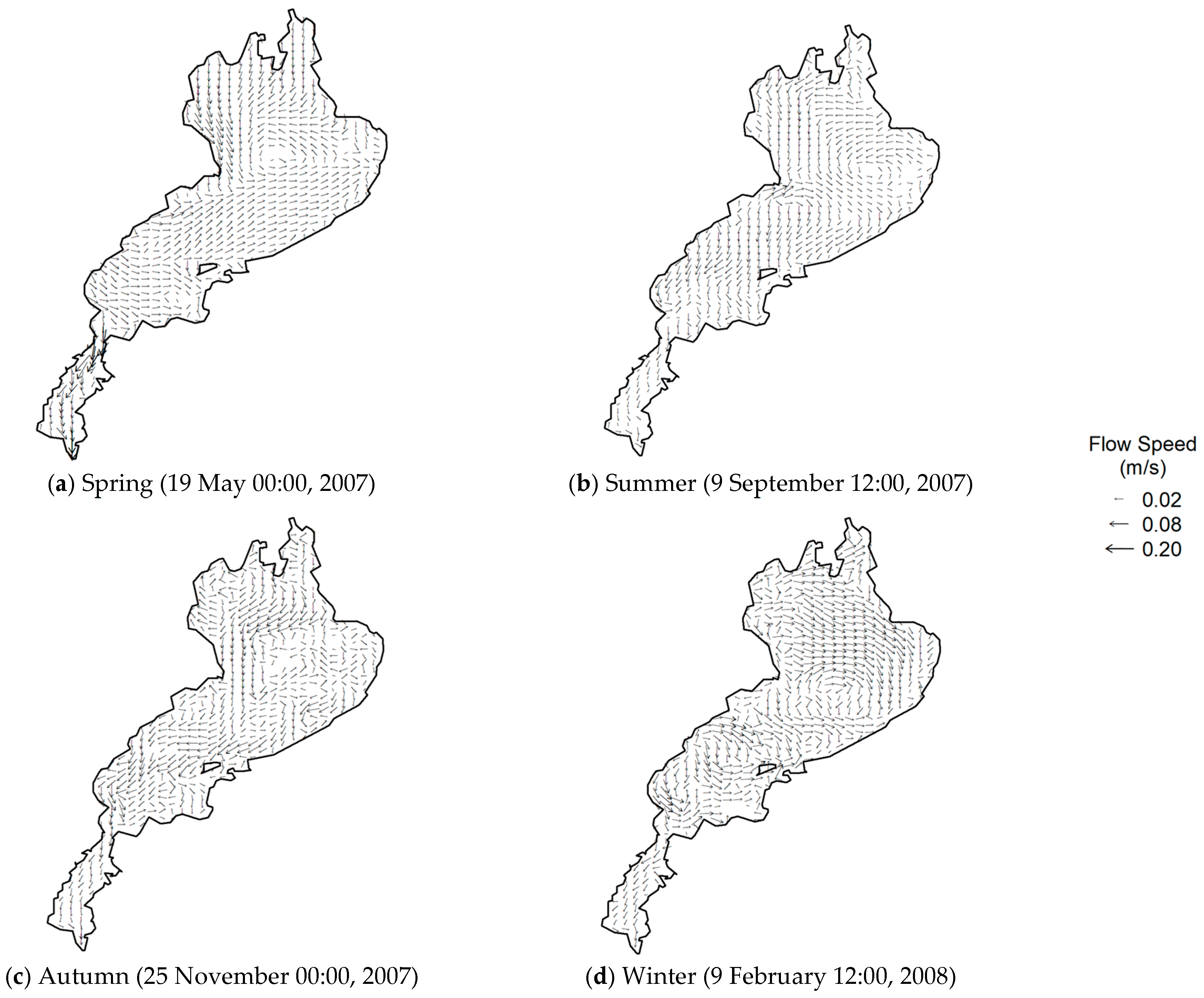
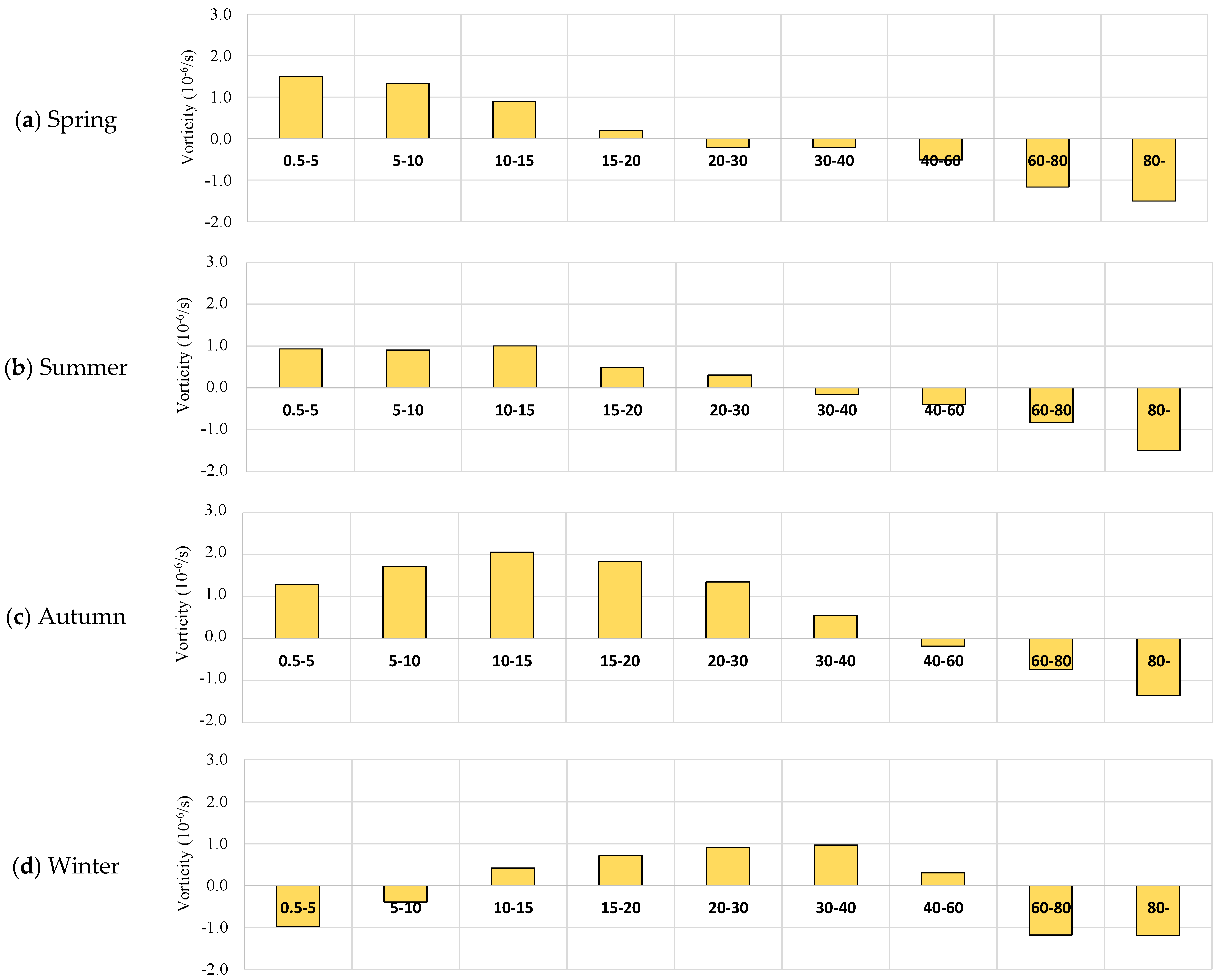
3.1. The Flow Field in the Case of Baseline Case

Figure 4 illustrates the representative surface flow fields for each season under baseline conditions using observed meteorological data. During the weakly stratified (spring) and stratified (summer) periods, a counterclockwise primary circulation with a maximum diameter of approximately 10 km forms at the lake’s center, with peak surface velocities reaching approximately 10–15 cm/s. Additionally, during the stratified (summer) season, a clockwise secondary circulation appears in the southwestern part of the lake, and a temporarily unstable tertiary circulation is also observed. In winter, a clockwise recirculation flow dominates across the lake.

Figure 5 presents the vertical distribution of vorticity (1/s) by season in the baseline case. The average vorticity values within the computational domain shown in Figure 3 were evaluated across nine depth layers: 0.5–5 m, 5–10 m, 10–15 m, 15–20 m, 20–30 m, 30–40 m, 40–60 m, 60–80 m, and deeper than 80 m. In the spring, the vorticity in the surface layer (0.5–15 m) is approximately 1.5 × 10⁻⁶ s⁻¹, with a dominant counterclockwise circulation. From summer to autumn, the positive vorticity intensifies and reaches a maximum of 2.0 × 10⁻⁶ s⁻¹ in the 20–30 m depth range near the thermocline. In winter, the vorticity becomes negative, and a clockwise gyre is formed at the surface with a vorticity of −1.0 × 10⁻⁶ s⁻¹. Below the thermocline (10–20 m depth), vorticity values of the opposite sign to those in the surface layer are observed, indicating a reversed circulation at depth.

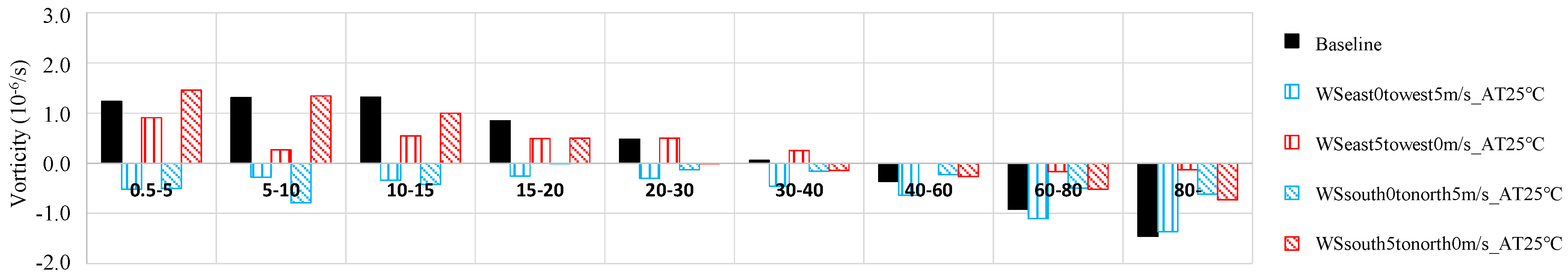
3.2. Wind-Driven Gyres: Directional Asymmetry and Topographic Modulation Under Spatially Varying Wind Fields

To investigate wind-driven circulation in Lake Biwa, numerical simulations were conducted by applying surface shear stress induced by spatially varying wind fields. The simulations were designed with linear wind speed gradients ranging from 5 m/s to 0 m/s, oriented either zonally (east–west) or meridionally (south–north). Four cases were considered based on combinations of wind direction and wind speed gradient orientation (see Table 1). For each case, seasonal variations in surface vorticity (units: s⁻¹) were evaluated.

Figure 6 shows the seasonally averaged (from spring to autumn) vorticity distributions for each scenario. The results reveal that in cases where counterclockwise wind stress vortices dominate—namely “WSeast5towest0m/s_AT25°C” and “WSsouth5tonorth0m/s_AT25°C”—the absolute values of vorticity peaked at 1.5 × 10⁻⁶ s⁻¹ and 2.0 × 10⁻⁶ s⁻¹, respectively. These elevated vorticity values are attributed to the greater shear gradient induced by the westerly wind compared to the southerly wind in the current configuration.

Conversely, in the clockwise vortex-dominated cases (“WSeast0towest5m/s_AT25°C” and “WSsouth0tonorth5m/s_AT25°C”), vorticity magnitudes were relatively lower, approximately −0.5 × 10⁻⁶ s⁻¹ and −1.0 × 10⁻⁶ s⁻¹, respectively. This asymmetry is not solely due to wind direction but also reflects the influence of lakebed topography. Specifically, the gentler slopes on the eastern and southern shores compared to the western and northern shores are hypothesized to affect both the development and intensity of the circulation patterns. This study qualitatively demonstrates the role of topographic asymmetry in enhancing or suppressing wind-driven vortices. In particular, the sloping bathymetry along the eastern and southern margins supports circulation retention through mechanisms analogous to topographic friction and steering effects [19].

Moreover, in the presence of counterclockwise wind stress vortices, a stronger and more stable horizontal circulation was consistently established compared to their clockwise counterparts. The larger vorticity magnitudes in these cases promoted the divergence of surface water masses, inducing upwelling in the central basin. This upwelling brings lighter surface waters to higher levels, enhancing vertical stratification and sustaining a stable circulation regime. Such conditions confer baroclinic stability to the lake’s vertical structure and are consistent with theoretical expectations for enclosed water bodies under wind forcing [8,17,20,21].

In contrast, clockwise wind stress vortices led to convergence at the lake center, triggering downwelling that advected denser waters upward. This vertical transport weakens stratification and reduces the overall stability of the circulation system.

Analysis of the vorticity structure within the thermocline (depths below 20 m) further revealed a compensatory deep flow opposite in direction to the surface current in counterclockwise cases. This counter-flow was associated with mean vorticity values in the range of −0.5 × 10⁻⁶ to −1.0 × 10⁻⁶ s⁻¹ and played a stabilizing role in the vertical circulation and stratification.

Together, these results underscore the importance of both wind stress asymmetry and lakebed morphology in modulating vorticity generation and circulation stability in enclosed lakes. In particular, cyclonic wind stress aligned with gently sloping shorelines promotes persistent, high-vorticity circulation regimes that enhance vertical stratification and reinforce large-scale gyres.

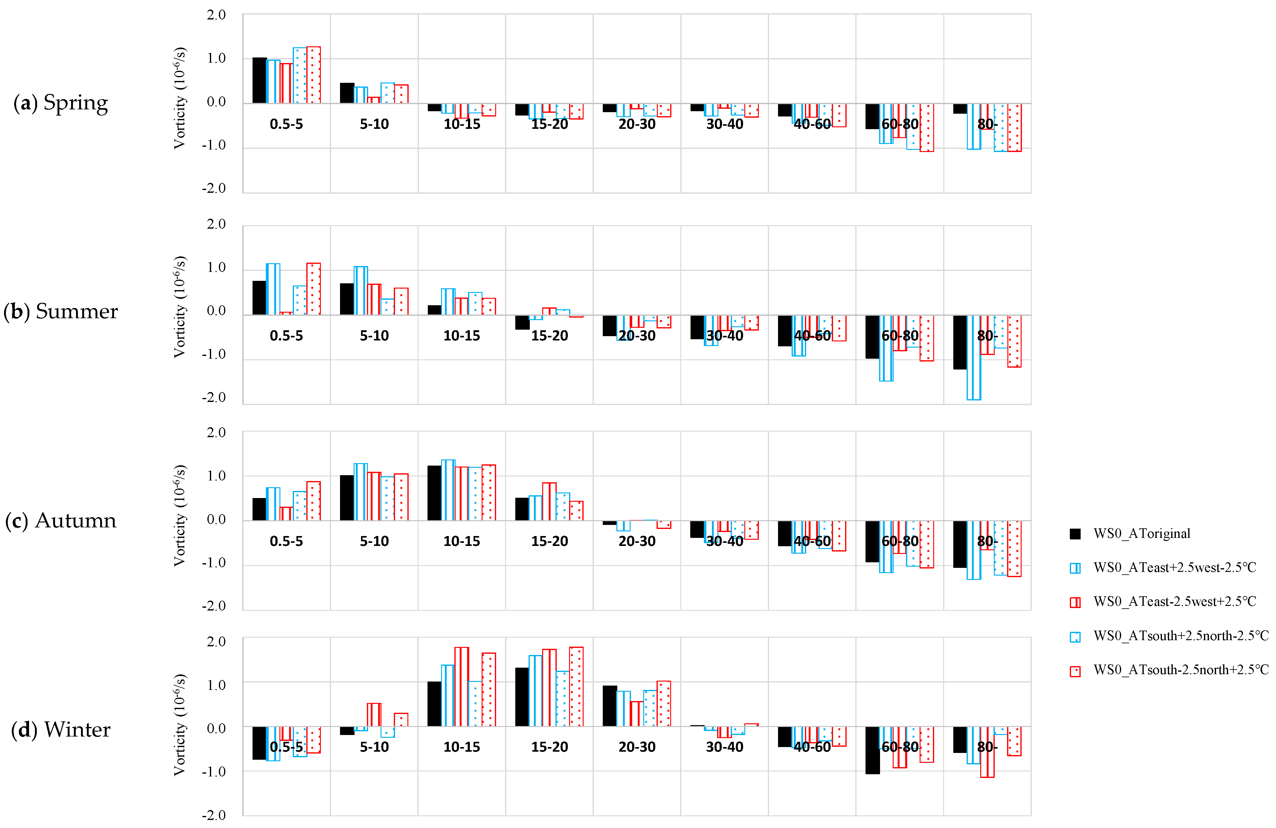
3.3. Thermal Gradient-Driven Gyres: Seasonal Reversals and Topographic Modulation Under Windless Conditions

To investigate lake circulation driven solely by thermal forcing, numerical simulations were conducted under windless conditions, thereby eliminating the influence of wind stress. In all simulations, the wind velocity within the computational domain was set to 0 m/s. Temperature distributions were prescribed based on observational data, and horizontal thermal gradients of ±2.5 °C were imposed. Four simulation cases were designed by applying these gradients in distinct directions: “WS0_ATeast+2.5west−2.5°C” (a gradient from east to west), “WS0_ATeast−2.5west+2.5°C” (west to east), “WS0_ATsouth+2.5north−2.5°C” (south to north), and “WS0_ATsouth−2.5north+2.5°C” (north to south).

Figure 7 presents the seasonal mean vorticity fields for each simulation case. In cases with an east–west thermal gradient, the north–south direction remained thermally uniform, and vice versa. Regardless of gradient direction, the simulations consistently revealed the development of cyclonic (counterclockwise) surface vorticity during spring, summer, and autumn and anticyclonic (clockwise) vorticity during winter.

This seasonal reversal of vorticity suggests the presence of thermally driven geostrophic circulation within the lake. Horizontal temperature gradients induce density gradients, generating pressure gradient forces. In the Northern Hemisphere, such pressure gradients are balanced by the Coriolis force, resulting in a flow that places warmer water masses to the left, thereby forming a cyclonic circulation. During winter, surface cooling promotes offshore-to-coastal flows, leading to the dominance of anticyclonic circulation.

In particular, during spring, summer, and autumn, coastal heating promotes vertical mixing and thermal accumulation near the shore, generating convergent flows from the shoreline to offshore. These flows intensify cyclonic surface vorticity. In contrast, divergent flows develop in winter, accompanied by anticyclonic surface vorticity. The Coriolis force acting on these flows is the principal driver behind the observed seasonal reversals in vorticity direction.

Although the direction of rotation was consistent across all simulation cases, the magnitude of vorticity varied depending on the orientation of the applied thermal gradient. In spring, summer, and autumn, stronger vorticity was observed in “WS0_ATeast+2.5west−2.5°C” compared to “WS0_ATeast−2.5west+2.5°C,” and in “WS0_ATsouth−2.5north+2.5°C” compared to “WS0_ATsouth+2.5north−2.5°C.” Quantitatively, peak surface vorticity reached 1.0 × 10⁻⁶ s⁻¹ in both “WS0_ATeast+2.5west−2.5°C” and “WS0_ATsouth−2.5north+2.5°C.” These cases correspond to warming along the eastern and southern shores, respectively, where gentle slopes and morphological asymmetry promote enhanced vertical mixing and local thermal accumulation, thereby strengthening convergence and the resulting geostrophic balance.

Conversely, in “WS0_ATeast−2.5west+2.5°C” and “WS0_ATsouth+2.5north−2.5°C,” the peak vorticity remained below 0.8 × 10⁻⁶ s⁻¹. This weakening is attributed to the topographic conditions along the western and northern shores, which suppress thermal accumulation and limit the development of strong thermal gradients and convergence zones.

Furthermore, the simulations revealed the formation of negative vorticity at depth during spring, summer, and autumn, ranging from −1.0 × 10⁻⁶ s⁻¹ to −2.0 × 10⁻⁶ s⁻¹. These subsurface anticyclonic flows appear to compensate for the cyclonic surface circulation. The transition depth between positive and negative vorticity was shallowest in spring, deepening through summer and autumn, and exceeded 30 m in some cases during autumn. This seasonal deepening reflects changes in the lake’s thermal stratification, with temperature differences extending to greater depths in autumn, thereby intensifying the deep counter-rotating flow.

In sum, these windless simulations demonstrate that horizontal temperature gradients alone can drive seasonally reversing circulation, with shoreline morphology modulating both intensity and spatial coherence. Enhanced thermal response along gently sloped shores generates stronger convergence, greater vorticity, and more robust stratification, even under spatially uniform heat input.

4. Conclusions

The mechanisms underlying wind- and thermally induced circulation in Lake Biwa were systematically evaluated through high-resolution numerical simulations. For the wind-driven cases, four scenarios were designed by applying linearly sheared wind stresses in both zonal and meridional directions, and seasonal mean vorticity distributions were analyzed. Maximum cyclonic vorticity reached 1.5 × 10⁻⁶ s⁻¹ (westerly winds) and 2.0 × 10⁻⁶ s⁻¹ (southerly winds) under conditions where cyclonic wind stress gradients dominated. These intensified responses were found to result from the combination of strong shear gradients and asymmetric lakebed topography. In contrast, under anticyclonic wind stress, markedly weaker vorticity was observed, and the spatial suppression of circulation was attributed not only to wind direction but also to the presence of steep slopes along the western and northern shores.

Under cyclonic forcing, strong horizontal gyres developed, producing surface divergence and associated upwelling in the lake center. This vertical structure contributed to enhanced stratification and increased baroclinic stability, accompanied by compensatory counter-flows in the deeper layers (−0.5 to −1.0 × 10⁻⁶ s⁻¹), which supported the overall stability of the circulation system. The results qualitatively demonstrated that both wind shear orientation and shoreline topography exert critical control on the strength and structure of wind-driven vorticity fields.

Thermally induced circulation was further evaluated by conducting windless simulations with imposed horizontal surface temperature gradients of ±2.5 °C in four configurations. From spring to autumn, cyclonic surface vorticity consistently emerged, whereas anticyclonic vorticity prevailed in winter. This seasonal reversal was consistent with the formation of geostrophic flows: convergent transport from coastal regions toward the center, induced by surface heating, enhanced cyclonic circulation during warmer months. Conversely, surface cooling in winter generated divergent flows, leading to anticyclonic circulation.

In scenarios where elevated temperatures were applied along the eastern and southern shores—regions characterized by gently sloping bathymetry—vorticity intensified up to 1.0 × 10⁻⁶ s⁻¹. These areas facilitated thermal accumulation and vertical mixing, promoting convergence and the development of strong cyclonic gyres. In contrast, thermal forcing along the steep western and northern shores yielded weaker responses (<0.8 × 10⁻⁶ s⁻¹), indicating suppression of convergence by steep bathymetry. In deeper layers, compensatory anticyclonic return flows (−1.0 to −2.0 × 10⁻⁶ s⁻¹) developed, with their vertical extent increasing seasonally, exceeding 30 m in autumn.

These findings revealed that shoreline slope asymmetry plays a pivotal role in shaping the formation and stability of both wind- and thermally driven circulations. In particular, the gently sloped southern and eastern shores were shown to promote convergence and upwelling, thereby enhancing internal circulation. While the simulations offer a conceptual framework for understanding how surface forcing interacts with bathymetry under idealized conditions, limitations such as the exclusion of hydrological inputs and the use of pseudo-weather forcing constrain its immediate predictive use. Nevertheless, the results provide a valuable diagnostic basis for future studies aiming to couple physical circulation with ecosystem processes, thereby informing more comprehensive models for lake management.

References

1. Cushman-Roisin, B.; Beckers, J.M. Introduction to Geophysical Fluid Dynamics: Physical and Numerical Aspects; Academic Press: Cambridge, MA, USA, 2011. [Google Scholar]
2. Bennington, V.; McKinley, G.A.; Kimura, N.; Wu, C.H. General circulation of Lake Superior: Mean, variability, and trends from 1979 to 2006. J. Geophys. Res. 2010, 115, C12015. [Google Scholar] [CrossRef]
3. Beletsky, D.; Schwab, D.J. Modeling circulation and thermal structure in Lake Michigan: Annual cycle and interannual variability. J. Geophys. Res. 2001, 106, 19745–19771. [Google Scholar] [CrossRef]
4. Huang, A.; Rao, Y.R.; Lu, Y.; Zhao, J. Hydrodynamic modeling of Lake Ontario: An intercomparison of three models. J. Geophys. Res. 2010, 115, C12076. [Google Scholar] [CrossRef]
5. Hamze-Ziabari, S.M.; Lemmin, U.; Foroughan, M.; Reiss, R.S.; Barry, D.A. Chimney-Like Intense Pelagic Upwelling in the Center of Basin-Scale Cyclonic Gyres in Large Lake Geneva. J. Geophys. Res. Ocean. 2023, 128, e2022JC019592. [Google Scholar] [CrossRef]
6. Stanev, E.V.; Chtirkova, B. Interannual change in mode waters: Case of the Black Sea. J. Geophys. Res. Ocean. 2021, 126, e2020JC016429. [Google Scholar] [CrossRef]
7. Oguz, T.; Besiktepe, S. Observations on the Rim Current structure, CIW formation and transport in the western Black Sea. Deep. Sea Res. Part I Oceanogr. Res. Pap. 1999, 46, 1733–1753. [Google Scholar] [CrossRef]
8. Ishikawa, K.; Kumagai, M.; Vincent, W.F.; Tsujimura, S.; Nakahara, H. Transport and accumulation of bloom-forming cyanobacteria in a large, mid-latitude lake: The gyre-Microcystis hypothesis. Limnology 2002, 3, 87–96. [Google Scholar] [CrossRef]
9. Imberger, J. Flux paths in a stratified lake: A review. In Physical Processes in Lakes and Oceans; American Geophysical Union: Washington, DC, USA, 1998; pp. 1–17. [Google Scholar]
10. Endoh, S. Diagnostic analysis of water circulations in Lake Biwa. J. Oceanogr. Soc. Jpn. 1978, 34, 250–260. [Google Scholar] [CrossRef]
11. Oonishi, Y. Development of the current induced by the topographic heat accumulation (I) The case of the axisymmetric basin. J. Oceanogr. Soc. Jpn. 1975, 31, 243–254. [Google Scholar] [CrossRef]
12. Lemmin, U. Insights into the dynamics of the deep hypolimnion of Lake Geneva as revealed by long-term temperature, oxygen, and current measurements. Limnol. Oceanogr. 2020, 65, 2092–2107. [Google Scholar] [CrossRef]
13. Reiss, R.S.; Lemmin, U.; Barry, D.A. Wind-induced hypolimnetic upwelling between the multi-depth basins of Lake Geneva during winter: An overlooked deepwater renewal mechanism? J. Geophys. Res. Ocean. 2022, 127, e2021JC018023. [Google Scholar] [CrossRef]
14. Reiss, R.S.; Lemmin, U.; Cimatoribus, A.A.; Barry, D.A. Wintertime Coastal Upwelling in Lake Geneva: An Efficient Transport Process for Deepwater Renewal in a Large, Deep Lake. J. Geophys. Res. Ocean. 2020, 125, e2020JC016095. [Google Scholar] [CrossRef]
15. MacIntyre, S.; Romero, J.R.; Kling, G.W. Spatial-temporal variability in surface layer deepening and lateral advection in an embayment of Lake Victoria, East Africa. Limnol. Oceanogr. 2002, 47, 656–671. [Google Scholar] [CrossRef]
16. Koue, J.; Shimadera, H.; Matsuo, T.; Kondo, A. Evaluation of Thermal Stratification and Flow Field Reproduced by a Three-Dimensional Hydrodynamic Model in Lake Biwa, Japan. Water 2018, 10, 47. [Google Scholar] [CrossRef]
17. Koue, J.; Shimadera, H.; Matsuo, T.; Kondo, A. Analysis of the effects of climate change on the gyre in Lake Biwa, Japan. J. Hydroinform. 2023, 25, 243–257. [Google Scholar] [CrossRef]
18. Kondo, J. Fundamentals of the surface heat balance. In Meteorology of Water Environment; Asakura Publishing: Tokyo, Japan, 1994; Chapter 6; pp. 132–159. (In Japanese) [Google Scholar]
19. Schwab, D.J.; Beletsky, D. Relative effects of wind stress curl, topography, and stratification on large-scale circulation in Lake Michigan. J. Geophys. Res. Ocean. 2003, 108, 3044. [Google Scholar] [CrossRef]
20. Csanady, G.T. Wind-induced barotropic motions in long lakes. J. Phys. Oceanogr. 1973, 3, 429–438. [Google Scholar] [CrossRef]
21. Gill, A.E. Atmosphere-Ocean Dynamics; Number 30 in International Geophysics Series; Academic Press: Cambridge, MA, USA, 1982. [Google Scholar]
Figure 1. Time changes in (a) air temperature and (b) wind speed at Hikone Meteorological Observatory.
Geosciences 15 00244 g001
Figure 2. Computational domain and bathymetry of Lake Biwa with a 500 m horizontal resolution.
Geosciences 15 00244 g002
Figure 3. Area for calculating the mean value of vorticity.
Geosciences 15 00244 g003
Figure 4. Surface flow field for each season in the baseline case.
Geosciences 15 00244 g004
Figure 5. Mean seasonal vorticity in the baseline case.
Geosciences 15 00244 g005
Figure 6. Mean vorticity in “Baseline”, “WS0_AT25°C”, “WSeast0towest5m/s_AT25°C”, “WSeast5towest0m/s_AT25°C”, “WSsouth0tonorth5m/s_AT25°C”, and “WSsouth5tonorth0m/s_AT25°C” cases.
Geosciences 15 00244 g006
Figure 7. Mean seasonal vorticity in “WS0_AToriginal”, “WS0_ATeast+2.5west−2.5°C”, “WS0_ATeast−2.5west+2.5°C”, “WS0_ATsouth+2.5north−2.5°C”, and “WS0_ATsouth−2.5north+2.5°C” cases.
Geosciences 15 00244 g007