Article

New Data from Minor Mountainous Lakes as High-Resolution Geological Archives of the Northern Apennines, Italy: Lake Moo

1
CNR-ISMAR—Consiglio Nazionale Delle Ricerca, Istituto di Scienze Marine, Via Gobetti 101, 40129 Bologna, Italy
2
Geological, Seismic and Soil Service, Emilia-Romagna Region, Viale Della Fiera 8, 40127 Bologna, Italy
*
Author to whom correspondence should be addressed.
Geosciences 2025, 15(6), 217; https://doi.org/10.3390/geosciences15060217
Submission received: 16 March 2025 / Revised: 28 May 2025 / Accepted: 8 June 2025 / Published: 11 June 2025
(This article belongs to the Section Hydrogeology)

Abstract

Sedimentary basins developed in mountain belts are natural traps of catchment erosion products and can produce comprehensive palaeoflood records that extend beyond instrumental or historical data. This study investigates the Lake Moo plain (1120 m a.s.l.), located in the Mt. Ragola (1712 m a.s.l.) ophiolitic massif in the Northern Apennines (Italy), which serves as an excellent case study for inferring the chronology of past flood events due to its position relative to the dominant atmospheric flow and its favorable geological and geomorphological characteristics. The Northern Apennines is a relatively understudied region regarding the reconstruction of past Holocene flood activity through the analysis of lake sediments and peat bogs, compared with areas like the Alps. The main objective of this research was to analyze sediment cores taken from a lake situated in a catchment area dominated by ultramafic rock lithologies and associated residual weathering cover deposits. This allowed us to detect and characterize past flood events in the Ligurian–Emilian Apennines. A multidisciplinary approach, integrated with reference data on geology, geomorphology, pedology, and petrography, enabled a more detailed description of the changes in the hydrologic cycle. Collectively, these data suggest that periods of increased past flood activity were closely linked to phases of rapid climate change at the scale of the Ligurian–Emilian Apennines. The preliminary results suggest that floods occurring during periods of temperature drops have distinct characteristics compared with those during temperature rises.

1. Introduction

Recent lake sediments [1,2,3,4,5,6,7,8,9,10,11,12,13,14,15] and fossil lacustrine deposits [16,17,18] have been extensively used as archives for reconstructing the recurrence rates and intensities of past flood events, alongside other proxies such as tree rings [19], speleothems [20,21], and alluvial fans and cones [22]. In this context, the Northern Apennines have received relatively less attention concerning Holocene flood activity. Only [23] provides a first overview of the periods of enhanced alluvial activity that occurred after the glacial retreat in the Apennine chain. The author’s data show that alluvial phases recorded at high altitudes are correlated with the expansion of the Alpine and Apennine glaciers and that their frequency and length varied during the Holocene. Furthermore, the correlation between the alluvial phases and climatic events recorded in the Northern Apennine seems to rule out a major role of the anthropogenic impacts, although present, on the environmental changes.
Until then, the peatlands in the Northern Apennines were mainly used to reconstruct vegetation dynamics. A comprehensive bibliographic review of the several palynological studies that document the main Holocene environmental dynamics of the Northern Apennines are within [24,25,26]. At higher altitudes, during the lower Holocene (between 13,500 and 10,500 B.P.) the landscape in the Northern Apennines was initially characterized by high pollen percentages of Pinus (sylvestris and uncinata) and subsequently by Betula. Between 10,500 and 6500 B.P., Abies dominated the woodlands and the vegetation remained stable until ca. 6500 cal B.P., when Abies pollen percentages showed an abrupt decrease and were slowly replaced by beech. This process was probably not synchronous in the region and began first in the east and proceeded successively to the west. According to [27], this westward shift in the beech tree is related to a change in air mass circulation patterns over the Northern Apennines. Then, the Fagus established itself at the treeline until today.
The region has experienced a series of localized extreme precipitation events in recent years, particularly in the ridge sector of the hydrographic basin, leading to significant flooding that has affected both urban and industrial centers in the plains (e.g., the Baganza valley flood on 12–13 October 2014 and the Nure–Trebbia–Ceno valleys flood on 13–14 September 2015). This study focuses on the Lake Moo plain (44°37′29″ N, 9°32′25″ E) in the upper Nure Valley in the Emilia Apennines (Figure 1), near the boundary between the Emilia-Romagna and Liguria regions (Piacenza province, Italy). This site was selected for its vulnerability to flooding, both during the Holocene [28,29] and more recently (September 2015), as several flood events originating from the streams flowing into the lake have also impacted the central plain area, including the lake basin. Geologically, the investigated area is dominated by the Mt. Ragola ophiolitic massif and strongly deformed clayey complexes belonging to the External Ligurides [30,31,32]. Finally, the Lake Moo area (Figure 1) is included in the Natura 2000 network, code IT4020008-ZSC-Monte Ragola, Lago Moò, Lago Bino [33], and has been classified as a geological site of regional importance [34].
The Lake Moo plain has been the subject of pollen stratigraphic research for local vegetation reconstructions [35]. In [35], the authors took a 13 m long sediment core, and the sediments were found to be barren of pollen above 4.40 m depth due to fluvial erosion and torrential transport. From the depths of 4.55 and 13.20 m, the obtained pollen diagram showed a low concentration and, therefore, the results must be considered indicative.
Only recently, after the 2015 flood that struck the study area, has the Lake Moo plain been the subject of new research [28,29]. This study was conducted in a very small catchment at altitudes above 1100 m a.s.l. to investigate how the hydrological cycle changes, induced by Holocene climatic oscillations, in this mountain sector of the Ligurian–Emilian Apennines. Based on different lab techniques, this work demonstrated that a multianalytical approach is necessary to detect past flood events from sediment cores taken from lakes located in catchment areas characterized by ophiolitic rock outcrops and associated residual weathering cover deposits, beyond the limits of historical and instrumental data.
To better identify the variability in sedimentation, magnetic susceptibility measurements, X-ray pictures, and non-destructive geochemical measurements using X-Ray Fluorescence Core Scanner (XRF-CS) were performed on the cores. X-ray fluorescence core scanning (XRF-CS) is a high-resolution, non-destructive geochemical technique used to analyze the elemental composition of sediment cores. It allows for the precise measurement of multiple elements across fine-scale sediment layers, providing valuable insights into sediment provenance and depositional processes. In the context of flood events, XRF-CS enables the identification of specific geochemical signatures associated with such events, distinguishing them from background sedimentation. The ability to scan cores at high resolution makes XRF-CS particularly effective for detecting rapid depositional events like floods, which often produce distinct geochemical patterns within the sediment record [36,37].

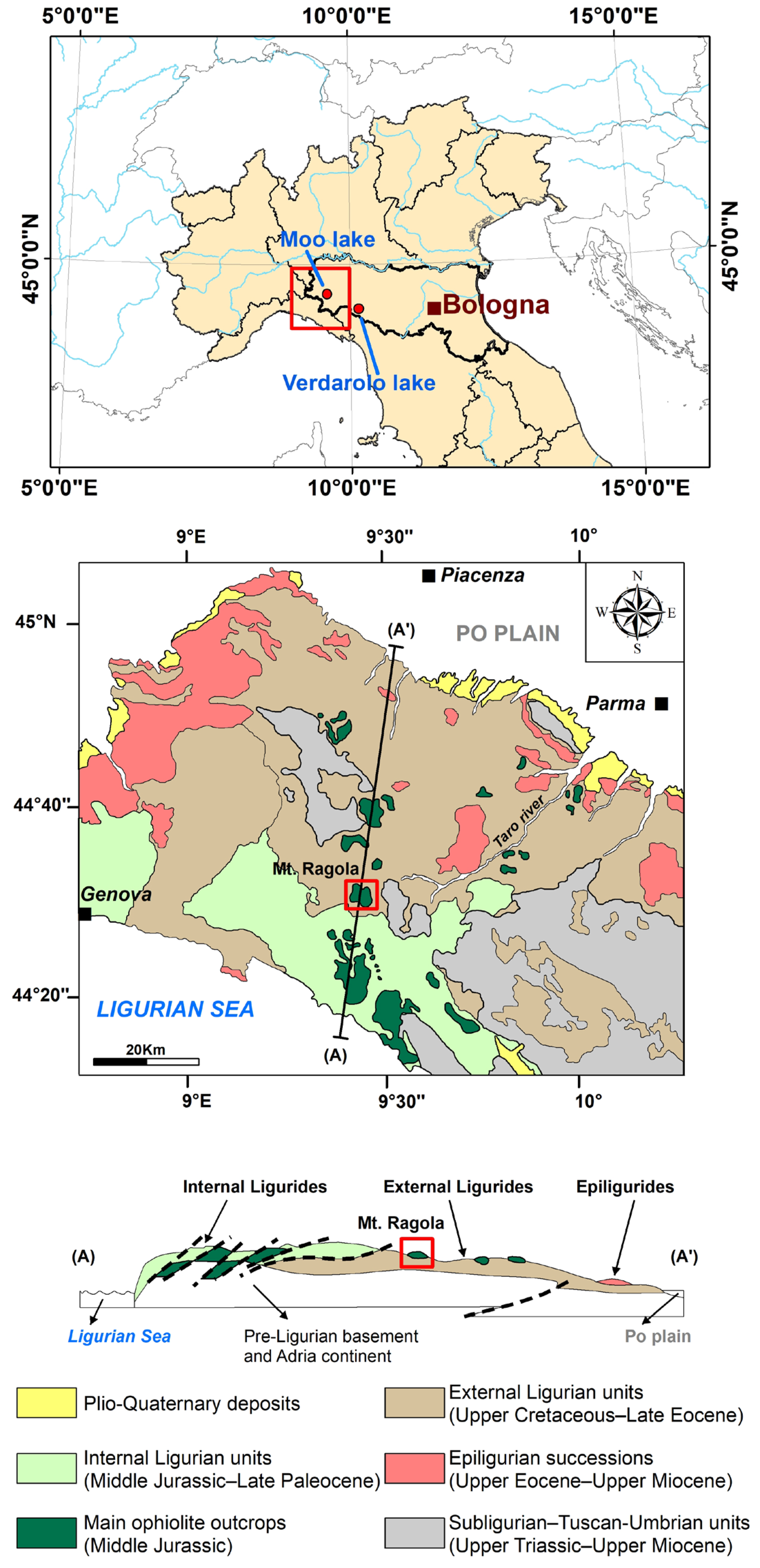
2. Geological and Geomorphological Setting

The study area is characterized by extensively deformed serpentinite masses of kilometer-sized dimensions that represent the accreted fragments of the Ligure–Piemontese oceanic basin separating the European and Adria plates during the Middle–Upper Jurassic [30,31] (Figure 2). Mt. Ragola consists of serpentinized mantle tectonites and appears as an orographic culmination of the External Ligurian units of the Northern Apennines [32]. The Mt. Ragola ultramafic massif covers an area of about 24 km2, is about 300 m thick, and is bordered by low-permeability deposits which are predominantly characterized by polygenic breccias (Mt. Ragola Complex, Late Santonian–Early Campanian [32], made of heterometric blocks of limestone or marly limestone embedded in a fine-grained matrix).
From a geomorphological point of view, the peatbog is in a depression formed by processes related to the Last Glacial Maximum [38]. On the other hand, [29] and the public database [39] interpreted the lake plain as the product of gravity processes mainly triggered by the incision of the Nure stream [32]. The geomorphology is likely enhanced by the superposition of lithological units with strong mechanical contrast, such as ophiolites and the underlying clayey unit [32]. The contact between these two units dips 5% toward the N–NE [29].
At the catchment scale, the ultramafic soils are commonly characterized by thicknesses ranging between a minimum of 15 cm and a maximum of 50 cm and poor horizon differentiation [40,41]. They are also defined as “AC soils” because the O horizon is commonly absent or a few millimeters thick and the poorly developed A horizon (topsoil) is directly in contact with the C horizon (subsoil). Cobbles and boulders are common throughout the entire profile. In the Lake Moo plain, marsh deposits (silty with occasional fine pebbles) are present and the organic matter is mostly concentrated at the top of the A horizon (topsoil) in the northeast sector and alluvial fan deposits (polygenic pebble–sand couplets) in the southern sector (Figure 3).
Considering the criteria indicated by references [3,6], Lake Moo shares several advantageous characteristics for the reconstruction of Holocene flood activity [28,29]:
-
Steep slopes (average inclination of 24°) composed of deposits highly susceptible to erosion (i.e., polygenic and monogenic breccias with a pelitic matrix—the Mt. Ragola Complex [32]);
-
Absence of lacustrine basins in the upstream part of the catchment;
-
Small drainage basin area (1.94 km2);
-
One dominant inflow into the lake;
-
Lack of regulated flow structures;
-
Lack of natural pre-lake sediment storage zones.
All these features make Lake Moo an ideal site to investigate past flood changes in the mountain sector of the Ligurian–Emilian Apennines.

3. Materials and Methods

3.1. Geospatial Data

All territorial data are available in vector digital format, organized and managed in a database with two types of software:
(1) ESRI 2018 AcrGIS 10.6.1 Redlands, CA Environmental Systems Research Institute. All this information is georeferenced in RDN2008 UTM zone 32 N;
(2) A free and open-source geographic information system: QGIS 3.42.0 “Munster” and was released on 21 February 2025.
Orthophotographs and DEMs have been acquired by the Geological, Seismic, and Soil Service, analyzed in GIS environment (georeferenced to the RDN2008 UTM zone 32N), with colored orthophotographs from A.G.E.A., with a 30–50 cm average pixel size and pictures taken between May and June 2011.

3.2. Coring and Analytical Methods

The field work aimed to core into the sediments filling the basin of the Lake Moo plain. Once extracted, the sediment cores were transported to the laboratory, stored in a refrigerated cell, and sectioned for subsequent petrophysical and geochemical analyses.
The coring was performed using a motorized percussion corer with a micro-stratigraphic casing (Topcorer 40). A total of three sediment cores were extracted under saturated conditions, reaching depths of (C1) 311 cm, (C2) 553 cm, and (C3) 556 cm below the ground surface (Figure 3). The cores recovered continuously and without interruptions along the entire depth. Sediment compaction, caused by coring-induced compression and water loss due to the weight of the core itself, resulted in recoveries of (C1) 87%—271 cm, (C2) 75%—405 cm, and (C3) 81%—452 cm, respectively (Table 1).
The cores were sectioned into 1 m long segments and placed in PVC liners. Once the protective casing was opened, the cores were photographed and prepared for subsequent geochemical and petrophysical analyses performed at the CNR-ISMAR laboratories.
To better identify the variability in sedimentation, magnetic susceptibility measurements, X-ray projections, and non-destructive geochemical measurements using X-Ray Fluorescence Core Scanner (XRF-CS) were performed on the cores.
The magnetic susceptibility measurement was acquired using a 6 cm diameter Bartington induction loop with a 2 cm step and a 10 s reading time. The measured data is corrected for both the sensor diameter and the core diameter, as well as for the background value and instrument drift, by taking empty readings both before and during the scan, following the measurement standard of the paleomagnetism laboratory at ISMAR CNR, Bologna. A total of 557 magnetic susceptibility measurements were performed.
The X-ray images of each core segment were acquired by acquiring three successive, partially overlapping exposures. This data is important because the exposure of the cores to X-rays allows for the differentiation of areas with coarser-grained material from those with finer-grained material, even in regions not visible to the naked eye. In Figure 4, the X-ray images of the first segment (the deepest one) of the Lake Moo C2 core are shown as an example. In the X-ray images, the lighter areas correspond to the less “transparent” portions to X-rays, which are the coarser layers, while the darker areas represent the finer layers with a higher water content.
The XRF-CS is used to investigate the variability in the geochemical composition of stratigraphic sections for paleoenvironmental and paleoclimatic purposes, for the identification of paleosols or volcanic ash, to study the mobilization and re-precipitation of elements sensitive to redox conditions, and to assess the presence of trace metals. The laboratory is equipped with a third-generation Avaatech XRF-CS, enabling high-resolution scanning of induced fluorescence. X-ray fluorescence core scanning is a non-destructive, automated methodology that analyzes elements from Al to U in the periodic table over a wide range of concentrations (from ppm to 100%). It can measure cores split longitudinally, U-channels, rock sections, speleothems, and discrete samples, with a variable resolution between 1 cm and 0.1 mm. The maximum effective sample length is 1600 mm, with a maximum width of 140 mm. This analytical technique is highly efficient as it requires no sample treatment other than the preparation of a flat surface. The core scanner is also equipped with an ultra-high-resolution digital camera (up to 70 microns) that captures images in visible and ultraviolet light using specific software for color analysis.
XRF-CS geochemical measurements were conducted at the CNR-ISMAR Core Repository, in Bologna. A total of 3156 XRF measurements were performed on the extracted cores [C1 n.253(x3); C2 n.383(x3); C3 n.416(x3)]. For each core, given their length, it was decided to use a 1 cm spacing between measurements with an acquisition window of 1 cm, following the laboratory’s standard acquisition protocol. In this way, the entire length of the core was scanned, acquiring 3 exposures at different electrical voltages, each with different excitation times. The different applied voltages covered various elements in the periodic table, according to the following scheme:
1st scan: 10 s exposure, 10 kV, 400 μA for Al, Si, P, S, Cl, K, Ca, Ti, V, Cr, Mn, and Fe;
2nd scan: 20 s exposure, 30 kV, 400 μA for Fe, Co, Ni, Cu, Zn, Br, Rb, Sr, Zr, Mo, and Pb;
3rd scan: 35 s exposure, 50 kV, 450 μA for Ag, Cd, Sn, Te, and Ba.

3.3. Lake Sediment Coring and Paleoflood Reconstruction

To identify and interpret flood event layers in a sediment core, we employed a combination of visual and instrumental analyses. The first step involved a visual inspection of the core, followed by X-ray imaging, which highlighted the alternation between fine- and coarse-grained areas. An initial instrumental proxy for the floods was obtained through magnetic susceptibility, with peaks linked to significant variations in granulometry and composition. XRF-CS signals were then used to distinguish flood layers based on site-specific geochemical elements. Using geochemical data, trends in element concentrations and their ratios were analyzed, both confirming previous results and uncovering previously overlooked patterns. The use of element ratios allows for the analysis of the trends of these elements without considering the absolute compositional variations and the ‘noise’ effect from the variation in other elements. Additionally, using the natural logarithm of the ratio (ln[elemA/elemB]) to obtain the log ratio of element variations enables the linearization of relationships, normalizing the distribution and reducing the influence of outliers. The geochemical data collected with XRF-CS for detailed-scale analysis were analyzed based on the extensive bibliography [36,37,42] and, in detail, based on the results of studies on the effects of weathering on the mobility of elements in the same serpentinites, conducted in a nearby area [43]. Results from [43] highlight that the elements Ti, Ga, Al, and Zr are prevalently immobile. For prevalently to tendentially mobile elements, the degree of mobility increases in the following order: Mn and Cr = Fe < V and Zn and Co < Ni < Si < Mg < Ca. Instead of Zr/Ti and Zr/Rb ratios, commonly used in the literature [36,37,42] as proxies for grain size variation and flood identification, we found the Ni/Ti ratio is particularly useful, as it reflects the relationship between the relatively mobile Ni and the predominantly immobile Ti. The geologic age model of the three sediment cores is based on four newly acquired radiocarbon ages obtained at the ETH Zurich laboratory. Radiocarbon determinations were calibrated using OxCal v4.4.4 [44] and Atmospheric data IntCal20 from [45].

4. Results

4.1. Core Analysis

4.1.1. X-Ray Imaging

All three cores show large sectors that are opaque to X-rays, typically attributed to flood events, where higher energy allows the transport and subsequent deposition of coarser fragments and particles.
Core C3, the southernmost, displays two large sectors, approximately 80 cm in length, that are completely opaque to X-rays, appearing almost white, with a coarse composition tending towards gravel. Starting from the surface, there is a 10 cm layer transparent to X-rays, likely corresponding to the current soil. This is followed by approximately 70 cm of relatively continuous sand, appearing gray to X-rays. From 80 to 170 cm, the first white X-ray cluster of distinctly coarse material appears. This is followed by 20 cm of intercalated layers of sand and finer material. From 190 to 280 cm, the second white X-ray cluster of distinctly coarse material appears. After this, the core contains an intercalation of sandy and fine layers, continuing until the base of the core, which tends to become thinner with depth.
Core C1, positioned between the other two cores, shows coarse material clusters in which continuous white X-ray portions are interspersed with finer, gray X-ray sections. After the first 20 cm, which are the shallowest, the first of two coarser sectors, approximately 100 cm in length, begins. Here, distinctly coarse segments, entirely white to X-rays, are intercalated with grayish X-ray levels, comprising alternating lighter and darker layers. From 130 to 167 cm, a relatively continuous section of material that is transparent to X-rays is observed. A second cluster of coarse material develops between 167 and 180 cm where there is a very thin, white X-ray level of coarse material. From 210 cm to the bottom of the core, the third coarse cluster begins, which, as in the first, includes portions of distinctly coarse grain size material (white to X-rays) intercalated with less coarse, sandy levels (grayish to X-rays).
In core C2, the most distal, northernmost, and closest to the current lacustrine environment, three main coarse clusters are identified. In these sectors, the distinctly coarse, white X-ray material is limited to two segments of about 10 cm at the top of the two clusters. The first 110 cm of the core consists of fine material, which is relatively transparent to X-rays. From 110 to 200 cm, the first coarse cluster appears, with the coarsest material at the top, gradually transitioning to intercalated finer material, grayish to X-rays, towards the bottom. From 200 to 221 cm, a section composed of intercalated fine material follows. A second cluster of coarse material develops between 221 and 267 cm. Finally, from 315 to 350 cm, the third coarse cluster appears, with the coarsest material at the top, continuing with intercalated coarse and fine material, alternating between gray and dark layers.
In summary, all three cores show alternations of material from distinctly coarse to fine under X-rays. In all the cores, two main coarse grain size material clusters can be identified. The coarse clusters differ significantly between the cores. From south to north, the material transitions from being completely coarse to including more fine intercalations. The portions of coarse material decrease as one moves northward.

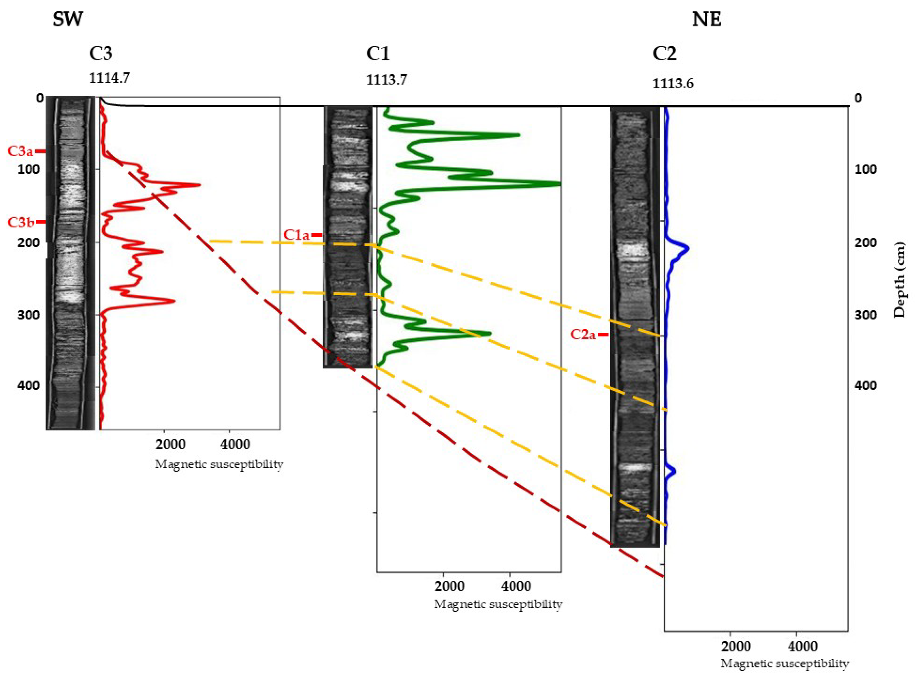
4.1.2. Magnetic Susceptibility Analysis

In all three cores, sectors are observed where peak values are recorded by the magnetic susceptibility curves. Values nearly an order of magnitude higher are found in the intermediate core C1 and the more southern core C3. The stratigraphic interval between the two clusters present in each core increases as one moves northward, towards the most distal core (Figure 5).

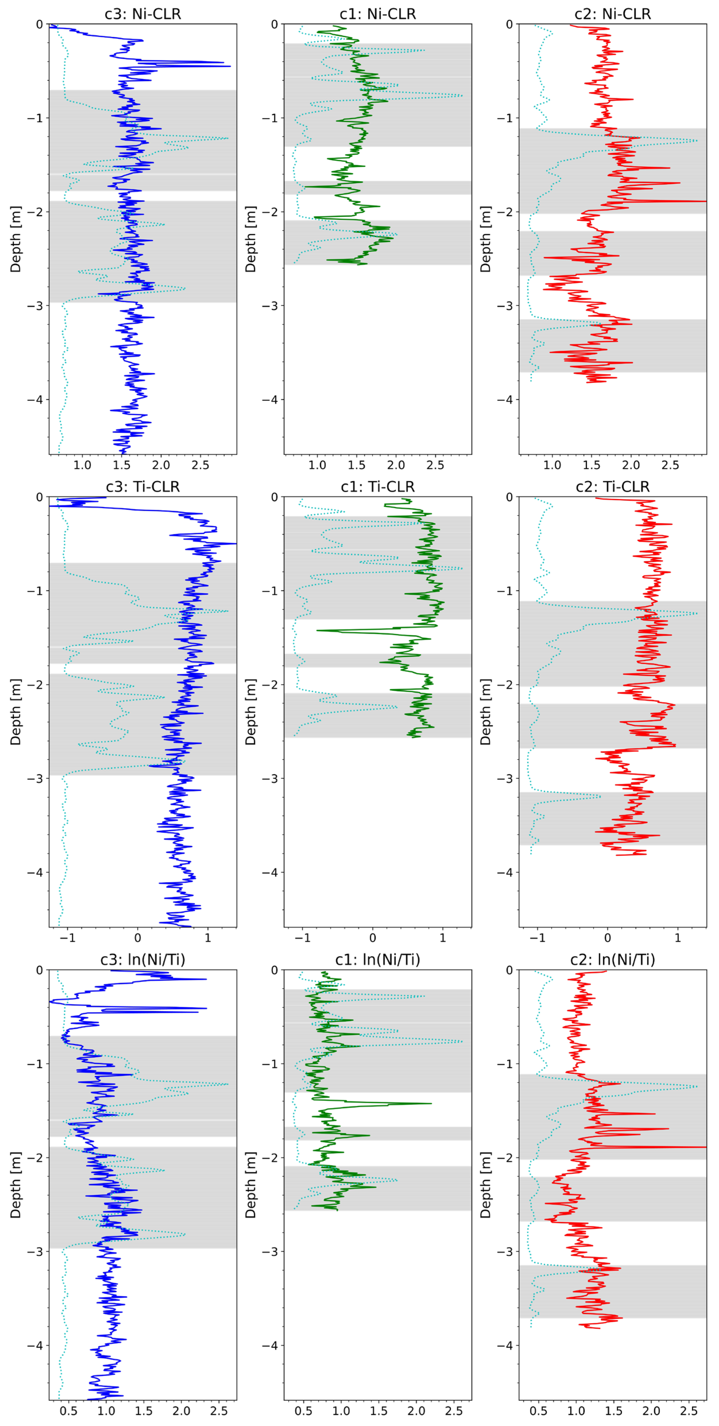
4.1.3. XRF Core Scanner

XRF signals can be used to discriminate flood layers among all identified event layers based on site-specific geochemical elements [36]. A single flood may be represented by multiple peaks in the element ratios because of the occurrence of multi-peaked rainfall events or the arrival at the site of flood peaks from the various sub-catchments at different times [42]. As this is valid in a medium–large basin with multiple sub-catchments, the same is valid in small basins where multiple peaks may represent a major climatic phase.
In lacustrine environments, elements like Al, Ti, and Rb are considered conservative. Their signal is least affected by changes in granulometry and provenance, and, therefore, they can be used as proxies for down-core variations in lithogenic particles relative to other components (organic matter, biogenic silica, carbonates, and other authigenic minerals) [37]. Based on the geology of the area and the associated geochemistry of weathering [43], the Ni/Ti ratio has proven particularly useful in identifying flood events, among other potential elements and ratios (Figure 6).
In C3 (left panel in Figure 6), Ni remains consistent across the entire core. A deviation is noticeable around 300 cm, at the base of the deepest coarse cluster. The two coarse segments (70–300 cm) show values with a positive trend compared with the deeper part of the core (>300 cm). Ti is quite homogeneous along the core, with higher values found in the coarse segments. It exhibits a decreasing trend towards the bottom of the core. The Ni/Ti ratio, which amplifies the signal variations in both elements, confirms the division of the core into the deeper, homogeneous part and the coarse part (<300 cm), where the geochemical signal can be interpreted as a proxy for the major flood phases.
In C1 (central panel in Figure 6), the Ni signal shows fluctuations with increasing trends in two coarser grain size clusters (20–120 cm and >210 cm). In the finer intermediate part, it exhibits a decreasing trend with spikes in the central coarse portion (167–180 cm). Ti shows a regular pattern in the two coarser grain size portions. In the intermediate portion there is a decrease in the signal. This decrease is mirrored by a relative increase in Ca, whose origin could be biogenic or authigenic rather than detrital, as there is also an increase in Br, whose variation is associated with the presence of organic matter. The Ni/Ti ratio shows a positive trend in the three coarser sectors. At the top of the coarse grain size cluster, starting from the bottom, there is an initial segment of approximately 30 cm with a fairly linear trend, followed by a triple of spikes, after which a short interval is followed by another spike. These secondary spikes may represent subsequent flood events within a major flood phase. The spike at around 140 cm, corresponding to a segment of very fine sedimentation and also present in the Ti signal, may reflect a localized response to an increase in organic matter and/or carbonates.
In C2 (right panel in Figure 6), the fluctuation of Ni mirrors the variation between the finer and coarser portions of the core. The upper meter is almost linear. At the top of the coarse grain size cluster, the signal increases to higher values, and the same pattern is observed in the other coarser sectors. Ti is almost linear up to the base of the first coarse block, and the intermediate coarse grain size cluster is clearly represented. After that, a sudden drop in the signal marks the transition to a finer portion, extending down to the deeper part of the core. The Ni/Ti ratio shows fluctuations due to the previous variations, clearly isolating the three coarser blocks. In the shallower block, the same pattern as the upper portion of C1 is observed, with a triple peak followed by a single peak.
More plots with trends in the depth of elements as detected with the XRF-CS are available in Chapter S1 of Supplementary Materials.

4.1.4. Dating

To verify possible correlations between the cores, the base of the upper flood phase of each core was dated using C-14. Organic material was sampled at 70 and 176.7 cm in C3, at 129.5 cm in C1, and at 200 cm in C2. Original data are available in Chapter S2 in Supplementary Materials and the position and dating (expressed in BP, before present) of the samples are shown in Table 2.

5. Discussion

The X-ray pictures of each core taken from the Lake Moo plain together with the magnetic susceptibility profiles and radiocarbon dating were used to create a stratigraphic section (Figure 7). The stratigraphic succession is characterized by clusters of coarse-grained deposits interbedded with organic-rich silty clays and peat layers. The geochemical data indicates distinct behavior between the C3 core and the C1–C2 cores, with differences in the distribution of elements with depth, particularly within the coarse layers that represent the flood phases (Figure 6).
An important unconformity identified from the geologic age model further supports the observations by [28,29]. This unconformity helps to explain why no pollen was found above 4.4 m depth [35]. Stratigraphic, geochemical, and geochronological data suggest that the flood events recorded in C3 are separate from those recorded in C1–C2 cores and, therefore, cannot be directly correlated. The depth of the unconformity is in accordance with the spill point altitude of Lake Moo (1114 m a.s.l.) [29].
The flood deposits identified in the three sediment cores were compared with the most relevant paleotemperature datasets available in the literature for the study area and the chronological period recorded in the Lake Moo sedimentary succession [46]. The Holocene paleoclimate reconstruction conducted by [46] for the nearby Lake Verdarolo represents a key reference. Lake Verdarolo is located at 1390 m a.s.l., 270 m higher and 54 km southeast of Lake Moo, in a climatically similar context (Figure 2). The authors reconstructed the mean July air temperature using a chironomid-based inference model, developed from data extracted from more than 200 lakes in Norway and the Swiss Alps [46]. This vegetation-independent paleotemperature reconstruction is the first for the Northern Apennines and is consistent with other records from central Italy [46].
The chronological data C1a (556–520 B.P.), C2a (514–310 B.P.), and C3b (4860–4656 B.P.) are shown alongside the reconstructed mean July air temperature from Lake Verdarolo (Figure 8) [46]. The chronological data from the cores (C1a; C1b; and C3b), as presented in Figure 8, indicates the intervals during which increased flooding occurred, specifically at the base of the stratigraphically uppermost coarse layer in C3, C2, and C1.
Comparing the ages of the flood activation phases (C1a, C2a, and C3b) with local air temperature variations (Figure 8) enables the correlation of different flood phases with specific climatic stages. The upper flood phase in C3 correlates with the temperature drop following the end of the Holocene Climate Optimum (HCO), indicated by the purple square in Figure 8. During this phase, the flood deposits are more massive and coarser (amalgamated layers), with fewer fine-grained sediments. In contrast, the flood phases in C1 and C2 are characterized by intercalations of fine and intermediate granulometry, with limited intercalations of coarse sediment levels. The Ni and Ti signal shows minimal fluctuations in C3 but greater fluctuations in C1 and C2. The Ni/Ti ratio, reflecting the relationship between the relatively mobile Ni and the predominantly immobile Ti [43], spikes during major flood events and highlights these phases. Additionally, the magnetic susceptibility curve trends closely with the main cluster of coarse sediment layers, further supporting the identification of major flood events.
As indicated in the literature [28,29], additional chronological data on the increased frequency of past flood events in the study area can be integrated with the reconstructed air temperatures presented in Figure 8. These combined data highlight the following:
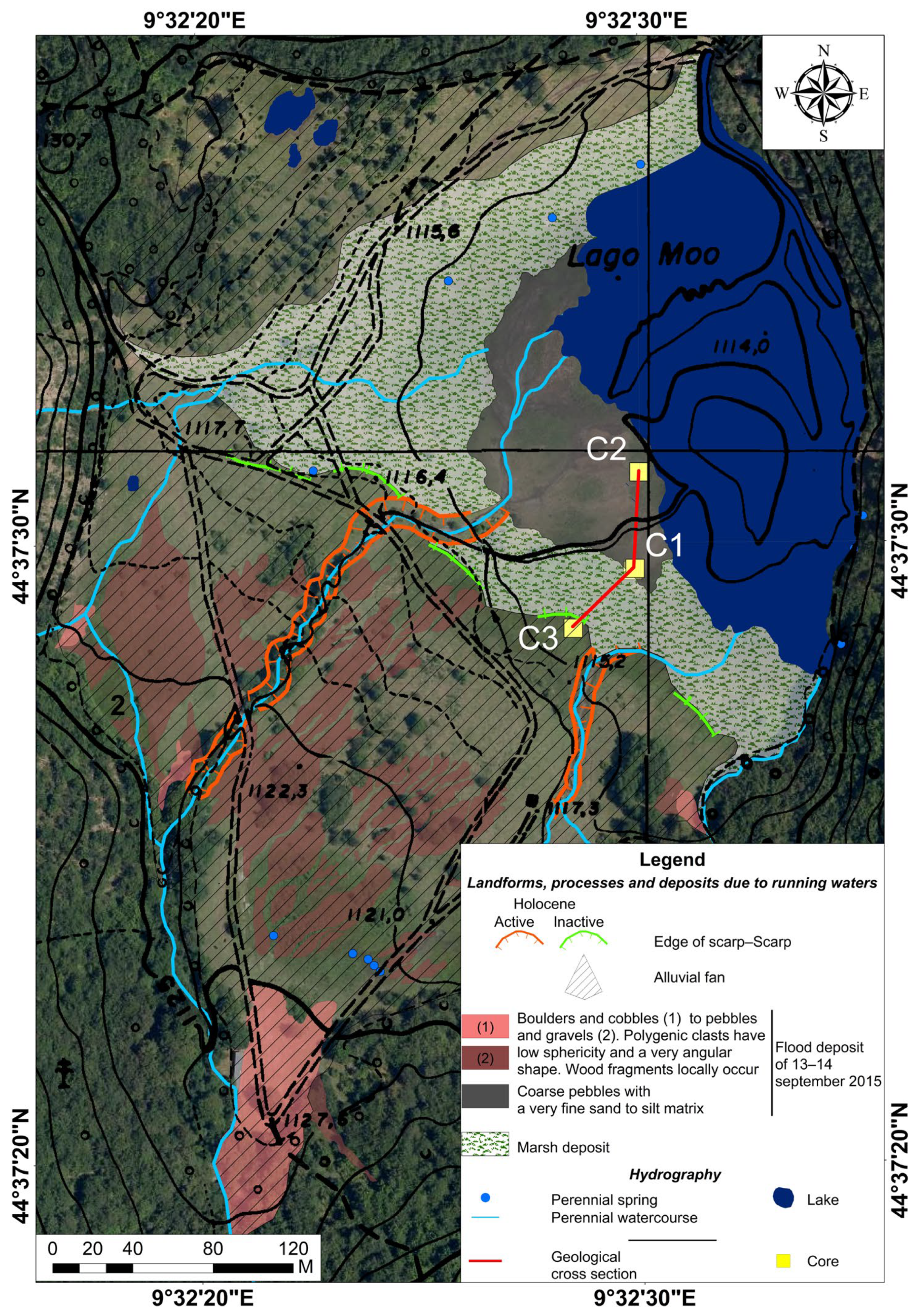
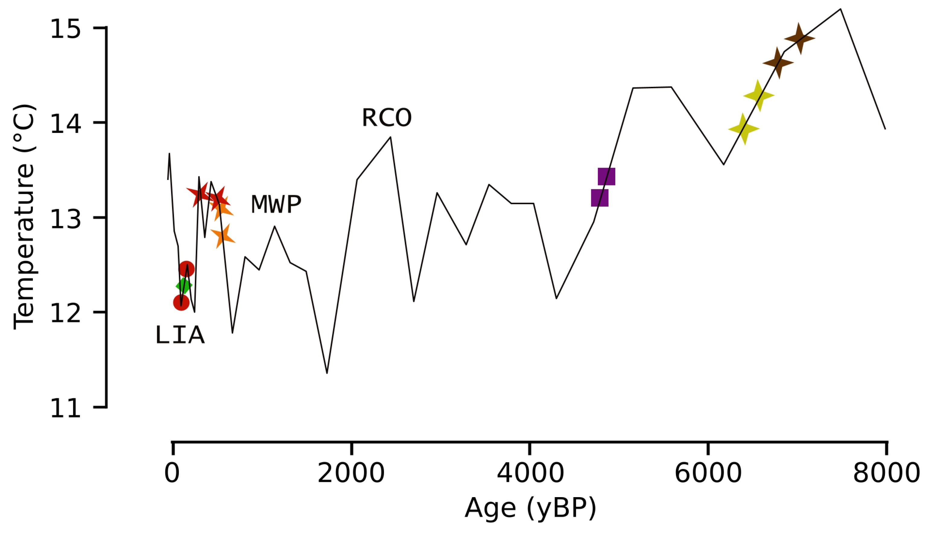
  • During the final phase of the Little Ice Age (LIA), the study area experienced several flood events (highlighted by the orange circle and green rhombus in Figure 8), which notably altered the morphology of the Lake Moo plain.
  • In agreement with the observations from the S1 borehole extracted in July 2017 at the Lake Moo plain [28], two distinct clusters of coarse material are evident at the end of the Holocene Climatic Optimum (HCO) peak (green cross (S1a: 6573–6396 B.P.) and brown cross (S1b: 7027–6785 B.P.) in Figure 8).
  • The sedimentological characteristics of samples (S1a) and (S1b) from [28] are similar to sample C3b in the present study.
At the scale of the Lake Moo plain, these data suggest that periods of increased flood activity correspond to phases of rapid Holocene climatic variability, as observed by [23] and may be associated with a pluvial phase. The analysis of historical cartography [29] reveals a series of flood events that occurred between 1828 and 1860, associated with cold and humid climatic conditions [47], during a marked temperature decline before the last peak of the Little Ice Age. Two additional wetter pluvial phases were proposed by [48]: the first at the beginning of the Sub-Atlantic period (2467 to 2728 B.P.), and the second phase in the Sub-boreal period (5000 to 4000 B.P.). The latter coincides with the increase in flood activity observed in core C3 (C3b: 4860–4656 B.P.) and is contemporaneous with a temperature decline, while the former corresponds to a period of rapid warming at the onset of the Roman Climatic Optimum (RCO). For the floods observed in C1 and C2, we hypothesize that they are related to a pluvial phase with a relative increase in temperature before the LIA temperature drop.
O6ther paleoclimate records from the Northern Apennines suggest different pluvial phases during the Holocene [21,49]. The first [21], identified in the Apuan Alps, through the stable isotope record (δ 18O) from a speleothem of the Corchia Cave in central–northern Italy, reveals intensified precipitation between ca. 7900 and 7300 cal B.P., coinciding with a rapid rise in temperature shortly before the peak of the Holocene Thermal Maximum. Similarly [49], a stratigraphic and chronological study in the Grotta Renella (Apuan Alps, central Italy) reveals increased flood frequency between ca 8.2 and 7.1 ka. These two pluvial periods are in phase with the coarse-grained layers (S1a and S1b in Figure 8) observed in S1 core from [28].

6. Conclusions

These preliminary results suggest that flood events occurring during temperature decline exhibit different sedimentological and geochemical characteristics compared with those triggered during warming phases. Future research should aim to clarify how abrupt changes in climatic parameters—such as temperature and precipitation—during the Holocene influenced the geochemical and sedimentary signatures of flood deposits, as well as their potential to reshape the mountainous landscape. To provide broader regional significance to the findings from the Lake Moo plain, similar investigations should be extended to other lacustrine environments and natural archives (e.g., tree rings, speleothems, and torrential fans) across the Northern Apennines.
The methodological approach applied in this study highlights the importance of an integrated, catchment-scale characterization of the geological, geomorphological, pedological, and petrographic settings—particularly in areas dominated by ultramafic rocks outcrops and associated residual weathering deposits. A petrological study [43] on the weathering of serpentinized ultramafic rock proved essential for interpreting the vertical geochemical variations observed in the cores. This was key for establishing stratigraphic correlations and for reconstructing the differing behaviors of flood events during the Holocene climatic oscillations. These reconstructions were further supported by rapid and effective core cross-correlation techniques, including high-resolution sediment visual analysis and non-destructive proxy measurements such as magnetic susceptibility, X-ray imaging, and non-destructive geochemical measurements using X-ray fluorescence core scanners (XRF-CS).

Supplementary Materials

The following supporting information can be downloaded at: https://www.mdpi.com/article/10.3390/geosciences15060217/s1, Figure S1: Calibration of the conventional radiocarbon date of samples; Chapter S1: XRF-CS geochemical variations with depth Core1; Chapter S2: Radiocarbon data analysis.

Author Contributions

Conceptualization, Y.N. and S.S.; methodology, Y.N. and S.S.; software, Y.N. and S.S.; validation, Y.N. and S.S.; formal analysis, Y.N. and S.S.; investigation, Y.N. and S.S.; data curation, Y.N. and S.S.; writing—original draft preparation, Y.N. and S.S.; writing—review and editing, Y.N. and S.S.; visualization, Y.N. and S.S.; supervision, Y.N. and S.S.; project administration, Y.N. and S.S. All authors have read and agreed to the published version of the manuscript.

Funding

This research was funded by the Geological Survey of Emilia-Romagna Region (Viale della Fiera 8, Bologna, Italy), grant number 2422/2021.

Data Availability Statement

The original contributions presented in this study are included in the article and the Supplementary Materials. Further inquiries can be directed at the author.

Acknowledgments

The authors would like to thank Andrea Gallerani (CNR ISMAR) and Maria Teresa De Nardo (Geological Survey Emilia-Romagna Region) for their work, as well as the two institutions: CNR ISMAR, for the facilities, and the Geological Survey Emilia-Romagna Region, for the funds provided for this research.

Conflicts of Interest

The authors declare no conflicts of interest.

References

  1. Ahlborn, M.; Armon, M.; Ben Dor, Y.; Neugebauer, I.; Schwab, M.J.; Tjallingii, R.; Shoqeir, J.H.; Morin, E.; Enzel, Y.; Brauer, A. Increased frequency of torrential rainstorms during a regional late Holocene eastern Mediterranean drought. Quat. Res. 2018, 89, 425–431. [Google Scholar] [CrossRef]
  2. Giguet-Covex, C.; Arnaud, F.; Dirk, E.; Jérôme, P.; Laurent, M.; Pierre, F.; Fernand, D.; Pierre-Jérôme, R.; Bruno, W.; Jean-Jacques, D. Frequency and intensity of high-altitude floods over the last 3.5ka in northwestern French Alps (Lake Anterne). Quat. Res. 2012, 77, 12–22. [Google Scholar] [CrossRef]
  3. Gilli, A.; Anselmetti, F.S.; Glur, L.; Wirth, S.B. Lake Sediments as Archives of Recurrence Rates and Intensities of Past Flood Events. In Dating Torrential Processes on Fans and Cones. Advances in Global Change Research; Schneuwly-Bollschweiler, M., Markus, S., Florian, R.M., Eds.; Springer: Dordrecht, The Netherlands, 2013; Volume 47, pp. 225–242. [Google Scholar] [CrossRef]
  4. Glur, L.; Wirth, S.B.; Büntgen, U.; Gilli, A.; Haug, G.H.; Schär, C.; Beer, J.; Anselmetti, F.S. Frequent floods in the European Alps coincide with cooler periods of the past 2500 years. Nat. Sci. Rep. 2013, 3, 2770. [Google Scholar] [CrossRef]
  5. Longman, J.; Ersek, V.; Veres, D.; Salzmann, U. Detrital events and hydroclimate variability in the Romanian Carpathians during the mid-to-late Holocene. Quat. Sci. Rev. 2017, 167, 78–95. [Google Scholar] [CrossRef]
  6. Schillereff, D.; Chiverrell, R.C.; Macdonald, N.; Hooke, J.M. Flood stratigraphies in lake sediments: A review. Earth-Sci. Rev. 2014, 135, 17–37. [Google Scholar] [CrossRef]
  7. Stoffel, M.; Butler, D.R.; Corona, C. Mass movements and tree rings: A guide to dendrogeomorphic field sampling and dating. Geomorphology 2013, 200, 106–120. [Google Scholar] [CrossRef]
  8. Stoffel, M.; Wyzga, B.; Marston, R.A. Floods in mountain environments: A synthesis. Geomorphology 2016, 272, 1–9. [Google Scholar] [CrossRef]
  9. Swierczynski, T.; Ionita, M.; Pino, D. Using archives of past floods to estimate future flood hazards. Eos 2017, 98. [Google Scholar] [CrossRef]
  10. Wilhelm, B.; Arnaud, F.; Sabatier, P.; Crouzet, C.; Brisset, E.; Chaumillon, E.; Disnar, J.R.; Guiter, F.; Malet, E.; Reyss, J.L.; et al. 1400 years of extreme precipitation patterns over the Mediterranean French Alps and possible forcing mechanism. Quat. Res. 2012, 78, 1–12. [Google Scholar] [CrossRef]
  11. Wilhelm, B.; Ballesteros-Cànovas, J.A.; Macdonald, N.; Toonen, W.H.J.; Baker, V.; Barriendos, M.; Benito, G.; Brauer, A.; Corella, J.P.; Denniston, R.; et al. Interpreting historical, botanical, and geological evidence to aid preparations for future floods. WIREs Water 2018, 6, e1318. [Google Scholar] [CrossRef]
  12. Wirth, S.B. The Holocene Flood History of the Central Alps Reconstructed from Lacustrine Sediments: Frequency, Intensity and Controlling Climate Factors. Ph.D. Thesis, ETH Zürich Bibliography, Zürich, Switzerland, 2013; 179p. [Google Scholar] [CrossRef]
  13. Wirth, S.B.; Glur, L.; Gilli, A.; Anselmetti, F.S. Holocene flood frequency across the Central Alps—Solar forcing and evidence for variations in North Atlantic atmospheric circulation. Quat. Sci. Rev. 2013, 80, 112–128. [Google Scholar] [CrossRef]
  14. Sabatier, P.; Moernaut, J.; Bertrand, S.; Van Daele, M.; Kremer, K.; Chaumillon, E.; Arnaud, F. A Review of Event Deposits in Lake Sediments. Quaternary 2022, 5, 34. [Google Scholar] [CrossRef]
  15. Wilhelm, B.; Amann, B.; Corella, J.P.; Rapuc, W.; Giguet-Covex, C.; Merz, B.; Støren, E. Reconstructing Paleoflood Occurrence and Magnitude from Lake Sediments. Quaternary 2022, 5, 9. [Google Scholar] [CrossRef]
  16. Zavala, C.; Pan, S. Hyperpycnal flows and hyperpycnites: Origin and distinctive characteristics. Lithol. Reserv. 2018, 30, 1–27. [Google Scholar] [CrossRef]
  17. Zavala, C.; Ponce, J.J.; Arcuri, M.; Drittanti, D.; Freije, H.; Asensio, M. Ancient Lacustrine Hyperpycnites: A Depositional Model from a Case Study in the Rayoso Formation (Cretaceous) of West-Central Argentina. J. Sediment. Res. 2006, 76, 41–59. [Google Scholar] [CrossRef]
  18. Zavala, C.; Arcuri, M.; Di Meglio, M.; Gamero Diaz, H.; Contreras, C.A. Genetic Facies Tract for the Analysis of Sustained Hyperpycnal Flow Deposits. In Sediment Transfer from Shelf to Deep Water—Revisiting the Delivery System; Slatt, R.M., Zavala, C., Eds.; AAPG Studies in Geology; AAPG: Tulsa, OK, USA, 2012; Volume 61, pp. 31–51. [Google Scholar]
  19. Ballesteros-Cánovas, J.A.; Stoffel, M.; St. George, S.; Hirschboeck, K. A review of flood records from tree rings. Prog. Phys. Geogr. 2015, 39, 794–816. [Google Scholar] [CrossRef]
  20. Regattieri, E.; Zanchetta, G.; Drysdale, R.N.; Isola, I.; Hellstrom, J.C.; Dallai, L. Late glacial to Holocene trace element record (Ba, Mg, Sr) from Corchia Cave (Apuan Alps, central Italy): Paleoenvironmental implications. J. Quat. Sci. 2014, 29, 381–392. [Google Scholar] [CrossRef]
  21. Zanchetta, G.; Isola, I.; Piccini, L.; Dini, A. The Corchia Cave (Alpi Apuane) a 2 Ma long temporal window on the earth climate. Tech. Period. Natl. Geol. Surv. Italy–ISPRA Geol. Field Trips 2011, 3, 55. (In Italian) [Google Scholar] [CrossRef]
  22. Schneuwly-Bollschweiler, M.; Stoffel, M.; Rudolf-Miklau, F. Dating Torrential Processes on Fans and Cones. Methods and Their Application for Hazard and Risk Assessment, 1st ed.; Springer: Dordrecht, The Netherlands, 2013; p. 424. [Google Scholar] [CrossRef]
  23. Giraudi, C. Coarse sediments in Northern Apennine peat bogs and lakes: New data for the record of Holocene alluvial phases in peninsular Italy. Holocene 2014, 24, 932–943. [Google Scholar] [CrossRef]
  24. Vescovi, E.; Kaltenrieder, P.; Tinner, W. Late-Glacial and Holocene vegetation history of Pavullo nel Frignano (Northern Apennines, Italy). Rev. Palaeobot. Palynol. 2010, 160, 32–45. [Google Scholar] [CrossRef]
  25. Vescovi, E.; Ammann, B.; Ravazzi, C.; Tinner, W. A new Late-glacial and Holocene record of vegetation and fire history from Lago del Greppo, northern Apennines, Italy. Veget. Hist. Archaeobot. 2010, 19, 219–233. [Google Scholar] [CrossRef]
  26. Guido, M.A.; Molinari, C.; Moneta, V.; Branch, N.; Black, S.; Simmonds, M.; Stastney, P.; Montanari, C. Climate and vegetation dynamics of the Northern Apennines (Italy) during the Late Pleistocene and Holocene. Quat. Sci. Rev. 2020, 231, 106206. [Google Scholar] [CrossRef]
  27. Leonelli, G.; Chelli, A. Spatial distribution patterns of dated landslide events in the Northern Apennines in response to Holocene regional climatic changes. Catena 2024, 236, 107705. [Google Scholar] [CrossRef]
  28. Segadelli, S.; Grazzini, F.; Rossi, V.; Aguzzi, M.; Marvelli, S.; Marchesini, M.; Chelli, A.; Francese, R.; De Nardo, M.T.; Nanni, S. Changes in high-intensity precipitation on the northern Apennines (Italy) as revealed by multidisciplinary data over the last 9000 years. Clim. Past 2020, 16, 1547–1564. [Google Scholar] [CrossRef]
  29. Segadelli, S.; Ogata, K.; Cocuccioni, M.; Gambini, S.; Martelli, L.; Morandi, L.F.; Oppo, G. Holocene Evolution of Minor Mountain Lacustrine Basins in the Northern Apennines, Italy: The Lake Moo Case Study. Geosciences 2022, 12, 272. [Google Scholar] [CrossRef]
  30. Marroni, M.; Meneghini, F.; Pandolfi, L. Anatomy of the Ligure-Piemontese subduction system: Evidence from Late Cretaceous middle Eocene convergent margin deposits in the Northern Apennines, Italy. Int. Geol. Rev. 2010, 52, 1160–1192. [Google Scholar] [CrossRef]
  31. Marroni, M.; Meneghini, F.; Pandolfi, L. A revised subduction inception model to explain the Late Cretaceous, double-vergent orogeny in the precollisional western Tethys: Evidence from the Northern Apennines. Tectonics 2017, 36, 2227–2249. [Google Scholar] [CrossRef]
  32. Elter, P.; Ghiselli, F.; Marroni, M.; Ottria, G. Note Illustrative del Foglio 197 “Bobbio” della Carta Geologica d’Italia alla Scala 1:50.000; Istituto Poligrafico e Zecca dello Stato: Rome, Italy, 1997; p. 106. [Google Scholar]
  33. Natura 2000 Network. Emilia-Romagna Region. Available online: https://ambiente.regione.emilia-romagna.it/it/parchi-natura2000/rete-natura-2000/siti/it4020008 (accessed on 7 March 2025).
  34. Geological Heritage. Emilia-Romagna Region. Available online: https://ambiente.regione.emilia-romagna.it/it/geologia/servizi-e-strumenti/cartografie-webgis/patrimonio-geologico-e-geositi (accessed on 7 March 2025).
  35. Bragio, G.; Guido, M.A.; Montanari, C. Palaeovegetational evidence in the upper Nure Valley (Ligurian-Emilian Apennines, Northern Italy). Webbia 1991, 46, 173–185. [Google Scholar] [CrossRef]
  36. Rapuc, W.; Jacq, K.; Develle, A.L.; Sabatier, P.; Fanget, B.; Perrette, Y.; Coquin, D.; Debret, M.; Wilhelm, B.; Arnaud, F. XRF and hyperspectral analyses as an automatic way to detect flood events in sediment cores. Sediment. Geol. 2020, 409, 105776. [Google Scholar] [CrossRef]
  37. Bertrand, S.; Tjallingii, R.; Kylander, M.E.; Wilhelm, B.; Roberts, S.J.; Arnaud, F.; Bindler, R. Inorganic geochemistry of lake sediments: A review of analytical techniques and guidelines for data interpretation. Earth-Sci. Rev. 2024, 249, 104639. [Google Scholar] [CrossRef]
  38. Marchetti, G.; Fraccia, R. Carta geomorfologica dell’alta Val Nure, Appennino piacentino, Scala 1:25.000. In Il Paesaggio Fisico dell’Alto Appennino Emiliano, Regione Emilia-Romagna; Carton, A., Panizza, M., Eds.; Grafis Edizioni: Bologna, Italy, 1988; p. 182. [Google Scholar]
  39. Geological, Seismic and Soil Service of the Emilia-Romagna Region: Landslide Characteristics in Emilia-Romagna. Available online: https://datacatalog.regione.emilia-romagna.it/catalogCTA/dataset/r_emiro_2013-06-17t184214 (accessed on 7 March 2020).
  40. Cortesogno, L.; Mazzucotelli, A.; Vannucci, R. Alcuni esempi di pedogenesi su rocce ultrafemiche in clima mediterraneo. Ofioliti 1979, 4, 295–312. (In Italian) [Google Scholar]
  41. Geological, Seismic and Soil Service of the Emilia-Romagna Region: Catalogue of Soil Maps and Derived Thematic Maps. Available online: https://ambiente.regione.emilia-romagna.it/en/geologia/soil/soil-knowledge/cartography (accessed on 22 April 2025).
  42. Turner, J.; Jones, A.; Brewer, P.; Macklin, M.; Rassner, S. Micro-XRF Applications in Fluvial Sedimentary Environments of Britain and Ireland: Progress and Prospects. In Micro-XRF Studies of Sediment Cores. Developments in Paleoenvironmental Research; Croudace, I., Rothwell, R., Eds.; Springer: Dordrecht, The Netherlands, 2015; Volume 17. [Google Scholar] [CrossRef]
  43. Venturelli, G.; Contini, S.; Bonazzi, A.; Mangia, A. Weathering of ultramafic rocks and element mobility at Mt. Prinzera, Northern Apennines, Italy. Mineral. Mag. 1977, 61, 765–778. [Google Scholar] [CrossRef]
  44. Bronk Ramsey, C. Bayesian Analysis of Radiocarbon Dates. Radiocarbon 2009, 51, 337–360. [Google Scholar] [CrossRef]
  45. Büntgen, U.; Sakamoto, M.; Talamo, S.; Kromer, B.; Bard, E.; Grootes, P.M.; Guilderson, T.P.; Southon, J.R.; Edwards, R.L.; Friedrich, R.; et al. The IntCal20 Northern Hemisphere Radiocarbon Age Calibration Curve (0–55 cal kBP). Radiocarbon 2020, 62, 725–757. [Google Scholar] [CrossRef]
  46. Samartin, S.; Heiri, O.; Joos, F.; Renssen, H.; Franke, J.; Brönnimann, S.; Tinner, W. Warm Mediterranean mid-Holocene summers inferred from fossil midge assemblages. Nat. Geosci. 2017, 10, 207–212. [Google Scholar] [CrossRef]
  47. Soldati, M.; Borgatti, L.; Cavallin, A.; De Amicis, M.; Frigerio, S.; Giardino, M.; Mortara, G.; Pellegrini, G.B.; Ravazzi, C.; Surian, N.; et al. Geomorphological evolution of slopes and climate changes in northern Italy during the late Quaternary: Spatial and temporal distribution of landslides and landscape sensitivity implications. Geogr. Fis. Din. Quat. 2006, 29, 165–183. [Google Scholar]
  48. Bertolini, G. Radiocarbon dating on landslides in the Northern Apennines (Italy). In Landslides and Climate Changes; Taylor & Francis: London, UK, 2007; ISBN 978-0-415-44318-0. [Google Scholar]
  49. Zhornyak, L.V.; Zanchetta, G.; Drysdale, R.N.; Hellstrom, J.C.; Isola, I.; Regattieri, E.; Piccini, L.; Baneschi, I.; Couchoud, I. Stratigraphic evidence for a “pluvial phase” between ca 8200–7100 ka from Renella cave (Central Italy). Quat. Sci. Rev. 2011, 30, 409–417. [Google Scholar] [CrossRef]
Figure 1. View of the Lake Moo landscape from the southern side. The Lake Moo plain has a surface area of about 0.15 km2 and it is located at an average height of 1120 m a.s.l.
Geosciences 15 00217 g001
Figure 2. Tectonic sketch map and geological cross-section of the Northern Apennines [modified from [30]] with location of the study area (red box).
Geosciences 15 00217 g002
Figure 3. Coring site’s location at Lake Moo plain. The profile follows a NE–SW trend and orthogonally intersects inactive alluvial fan deposits. Base map data are from Regional Technical Map 1976, contour interval = 5 m.
Geosciences 15 00217 g003
Figure 4. Example of X-ray pictures of the Lake Moo C2 core—first segment (the deepest one). The lighter areas correspond to the less “transparent” portions to X-rays, which are the coarser layers. The blue references indicate the overlap between the first projection (core2_I_1) and the second projection (core2_I-2). The orange references indicate the overlap between the second projection (core2_I-2) and the third projection (core2_I-3); A = top; B = bottom.
Geosciences 15 00217 g004
Figure 5. Magnetic susceptibility fluctuation in cores. Vertical scale (cm) and horizontal scale (susceptibility) are the same for the three cores. Notice the very low values in the core C2 (in red) on right part of the image.
Geosciences 15 00217 g005
Figure 6. XRF-CS results for Ni, Ti, and the Ni/Ti ratio in C3 (blue), C1 (green), and C2 (red). Magnetic susceptibility fluctuations are shown in light blue, with the intensity scale varying among the three cores to highlight differences along the core. Gray shadows indicate the portions of each core that represent flood phases (see text). The base of the upper flood phase in each core was dated using C-14. Data for individual elements are represented as centered log ratios [37], while the ratios are shown as the natural logarithm (ln) of the ratio between elements expressed in cps (counts per second).
Geosciences 15 00217 g006
Figure 7. Schematic sections (not to scale) show the studied stratigraphic succession derived from the correlation of the three core sediments. The trace of cross-section is shown in Figure 3. Dashed line: unconformity. Horizontal and vertical scale, 1:200. C1a: 556–520 B.P., C2a: 514–310 B.P., C3a: 7–35 B.P., C3b: 4860–4656 B.P.
Geosciences 15 00217 g007
Figure 8. Comparison of the variation in July mean air temperature (black line), reconstructed from chironomid-inferred data at the Lake Verdarolo site (from [46] see Figure 2 for location), with the ages of the reconstructed floods from this study and the literature for the same area. From this study: purple square—bottom age of the uppermost coarse layer stratigraphically in C3 (C3b: 4860–4656 B.P.); orange cross—bottom age of the uppermost coarse layer stratigraphically in C1 (C1a: 556–520 B.P.); red cross—bottom age of the uppermost coarse layer stratigraphically in C2 (C2a: 514–310 B.P.). From [29], red circle and green rhombus—reconstructed from historical cartography. From [28], green cross (S1a: 6573–6396 B.P.) and brown cross (S1b: 7027–6785 B.P.). RCO: Roman Climatic Optimum, LIA: Little Ice Age, MWP: Medieval Warm Period.
Geosciences 15 00217 g008
Table 1. Summary table of the coring conducted at Lake Moo plain, including location (WGS84GDD), depth reached, length of the recovered core, and the corresponding percentage (recovery/depth). The length of the recovered core represents the entire depth of the coring. Its shorter length compared with the “depth” is due to coring-induced compaction and water loss caused by the weight of the core itself.
Core CodeLatitudeLongitudeDepth (cm)Recovery (cm)Recovery Percentage (%)
C144.624789.5416731127187%
C244.625249.5416655340575%
C344.624559.5412855645281%
Table 2. Full list of radiocarbon sample age and description details.
Core
Code
Core
Depth (cm)
MaterialCalibrated Age B.P.
(±2 Sigma)
Calibrated Range BC/AD
(±2 Sigma)
C3a70Woody
frustules
7–35
26–35
1957–1985 CE
1976–/1985 CE
C3b176.7Woody frustules4860–4656
4754–4716
4667–4656
2910–/2706 BCE
2804–/2766 BCE
2717–/2706 BCE
C2a200Rootlets514–3101436–/1640 CE
C1a129.5Rootlets624–600
556–520
1326–1350 CE
1394–/1430 CE
Disclaimer/Publisher’s Note: The statements, opinions and data contained in all publications are solely those of the individual author(s) and contributor(s) and not of MDPI and/or the editor(s). MDPI and/or the editor(s) disclaim responsibility for any injury to people or property resulting from any ideas, methods, instructions or products referred to in the content.

