
Comparative Analysis of IMERG Satellite Rainfall and Elevation as Covariates for Regionalizing Average and Extreme Rainfall Patterns in Greece by Means of Bilinear Surface Smoothing


Abstract
1. Introduction
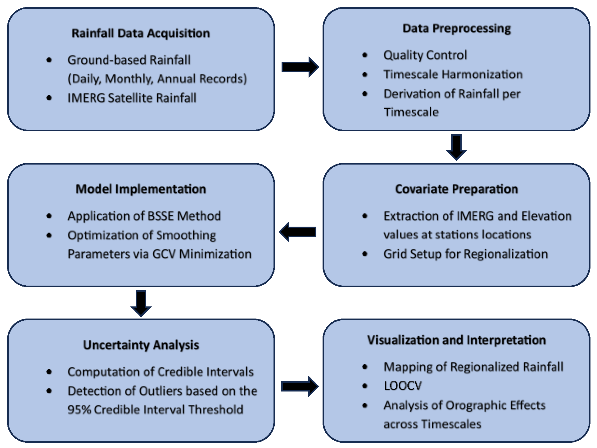
2. Methodology
2.1. Bilinear Surface Smoothing
2.2. Credible Intervals in the BSS Framework
2.2.1. Formulation Based on the BSS Framework
2.2.2. Computation of the Residual Sum of Squares
2.2.3. Estimation of the Error Variance
2.2.4. Posterior Covariance Matrix of the Fitted Surface and Credible Interval Assessment
2.3. Regionalization Performance Assessment
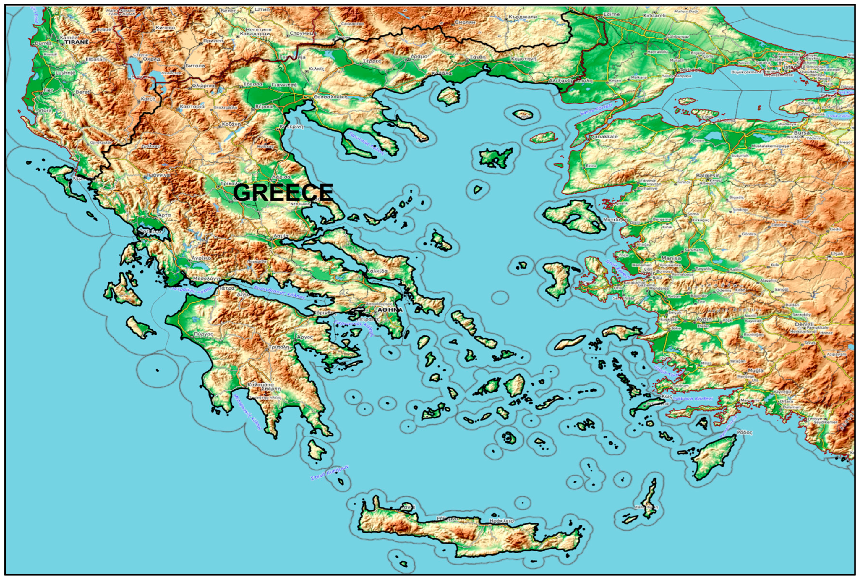
3. Study Area and Data
3.1. Study Area
3.2. Ground-Based Data
3.2.1. Daily and Monthly Records
- Stations with daily records: 61 rainfall series with over 60 years of data, 56 of which are sourced from the Hydroscope database (http://www.hydroscope.gr/, accessed on 10 February 2023) and 5 from the Greek Meteorological Service;
- Stations with monthly records within Greece: 31 rainfall series from the Global Historical Climatology Network (GHCN), each spanning more than 30 years;
- Stations with monthly records from neighboring countries: 36 stations from the GHCN, located in Turkey, North Macedonia, Bulgaria, and Albania, also with data spanning over 30 years.
3.2.2. Annual Maxima Records
- 503 daily rain gauges, with 130 situated at sites also equipped with a rain recorder;
- 280 rain recorders, providing sub-daily resolution data.
3.3. Satellite Data
3.4. Elevation Data
4. Results and Discussion
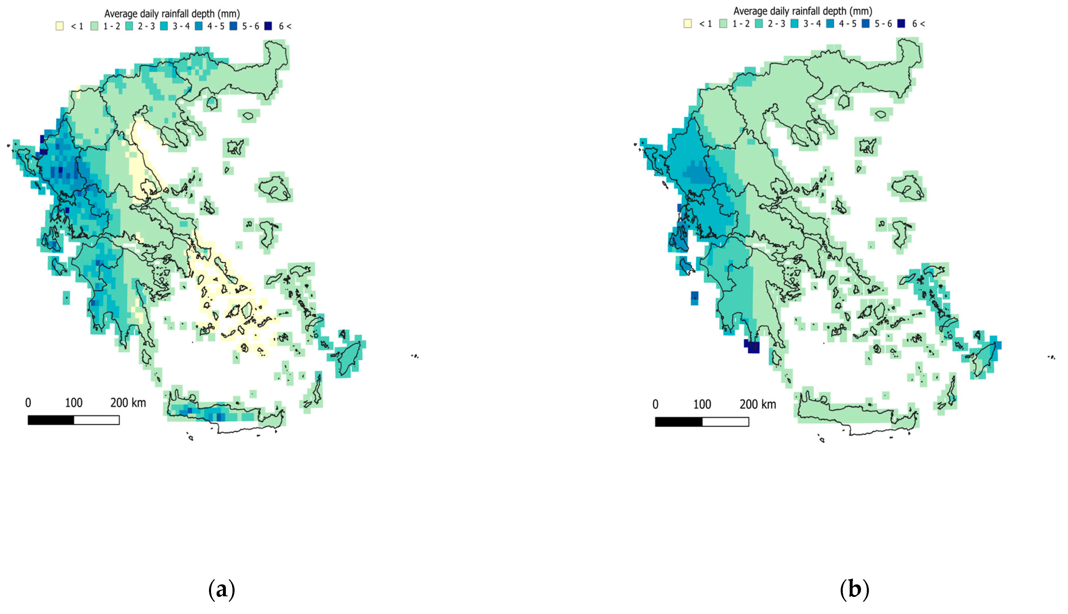
4.1. Regionalization of Average Daily Rainfall
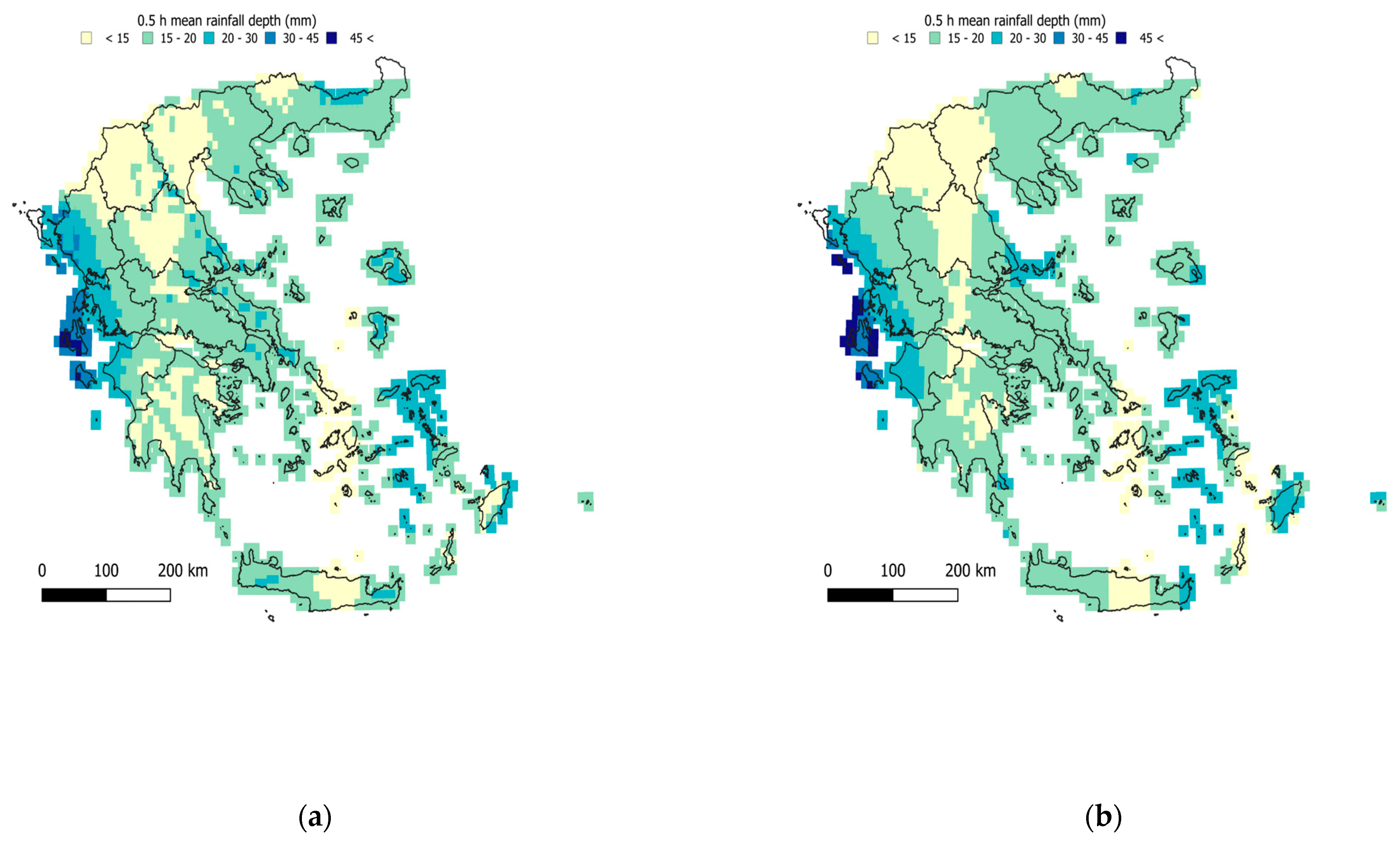
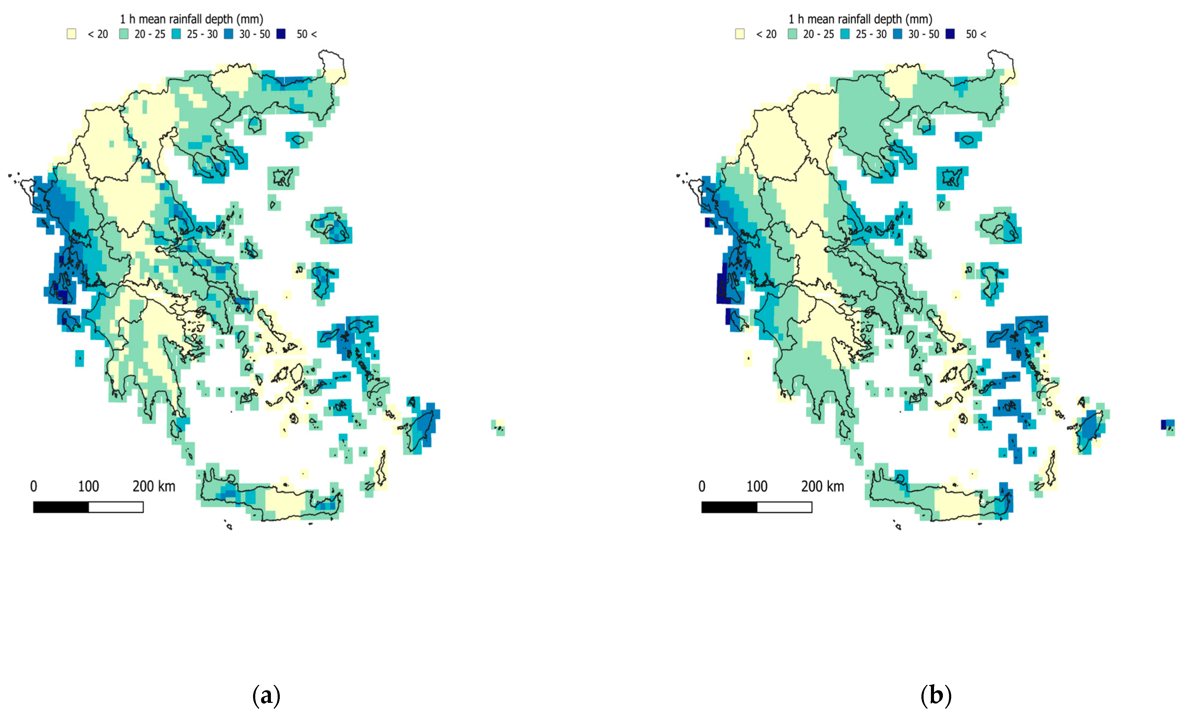
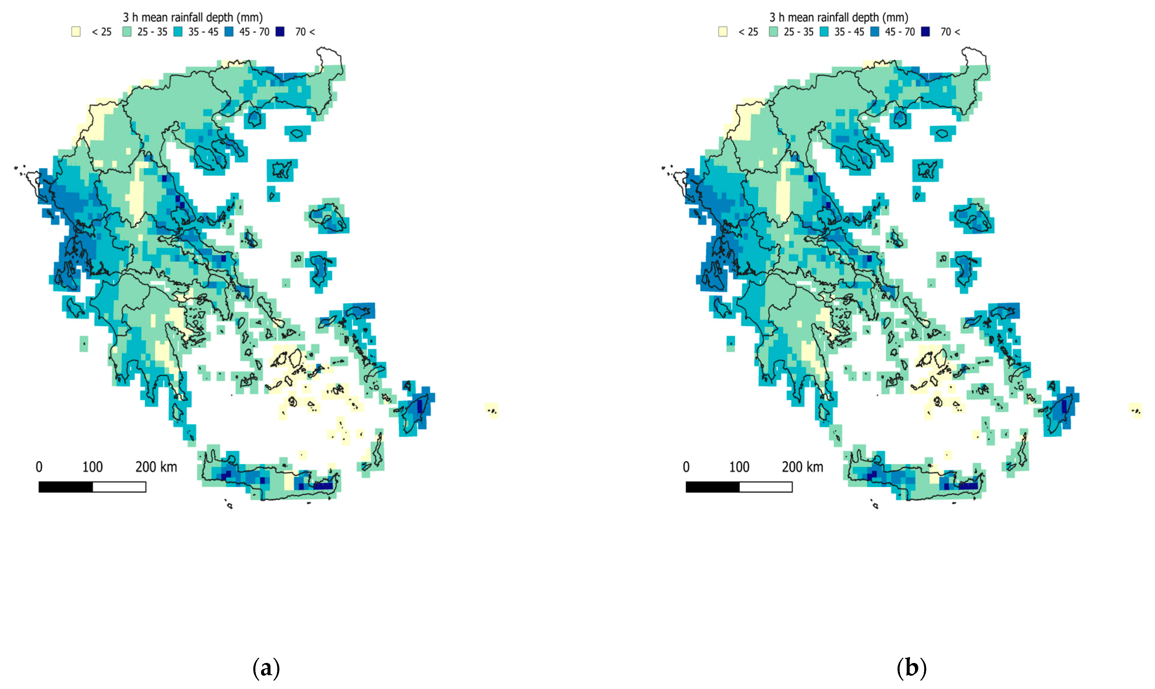
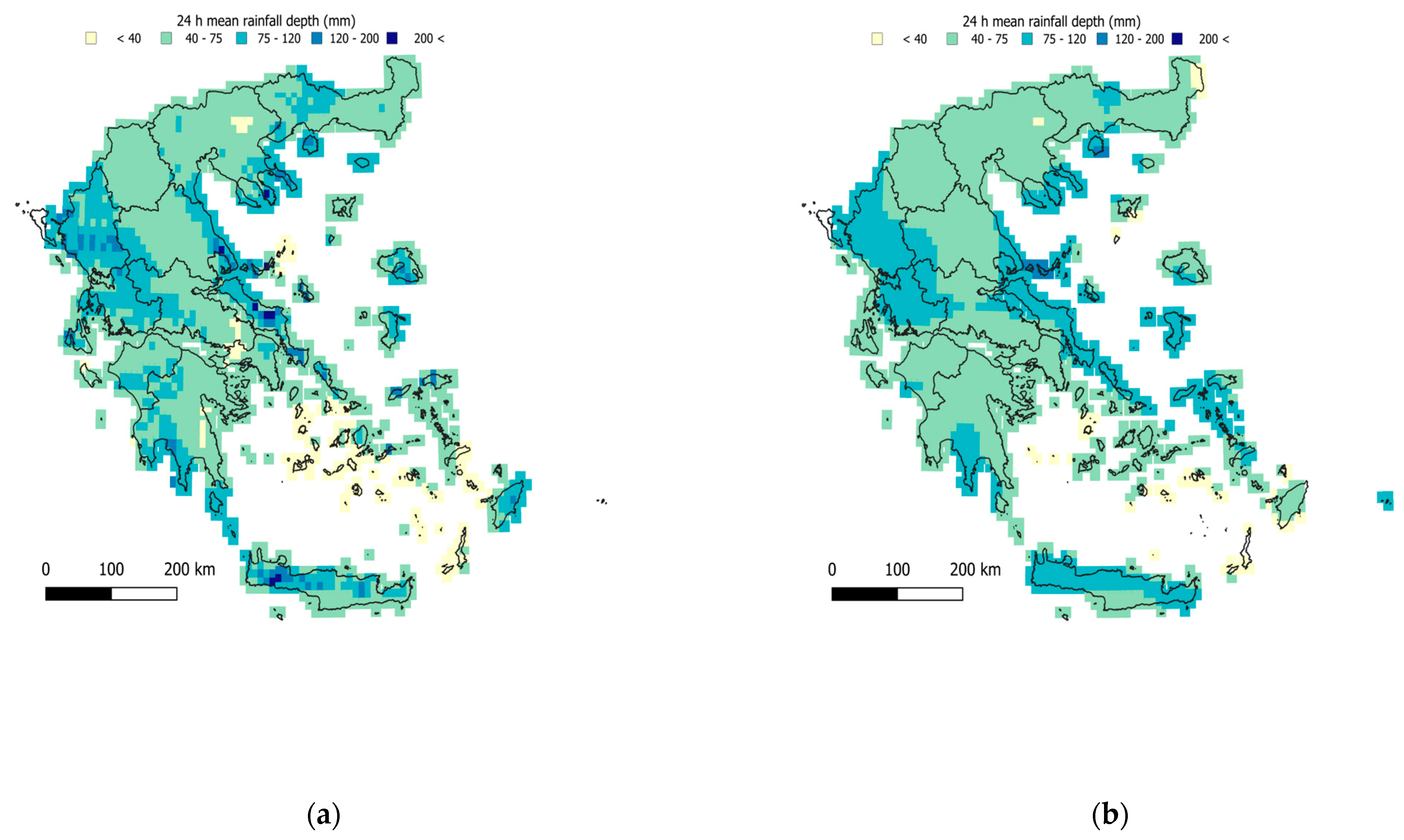
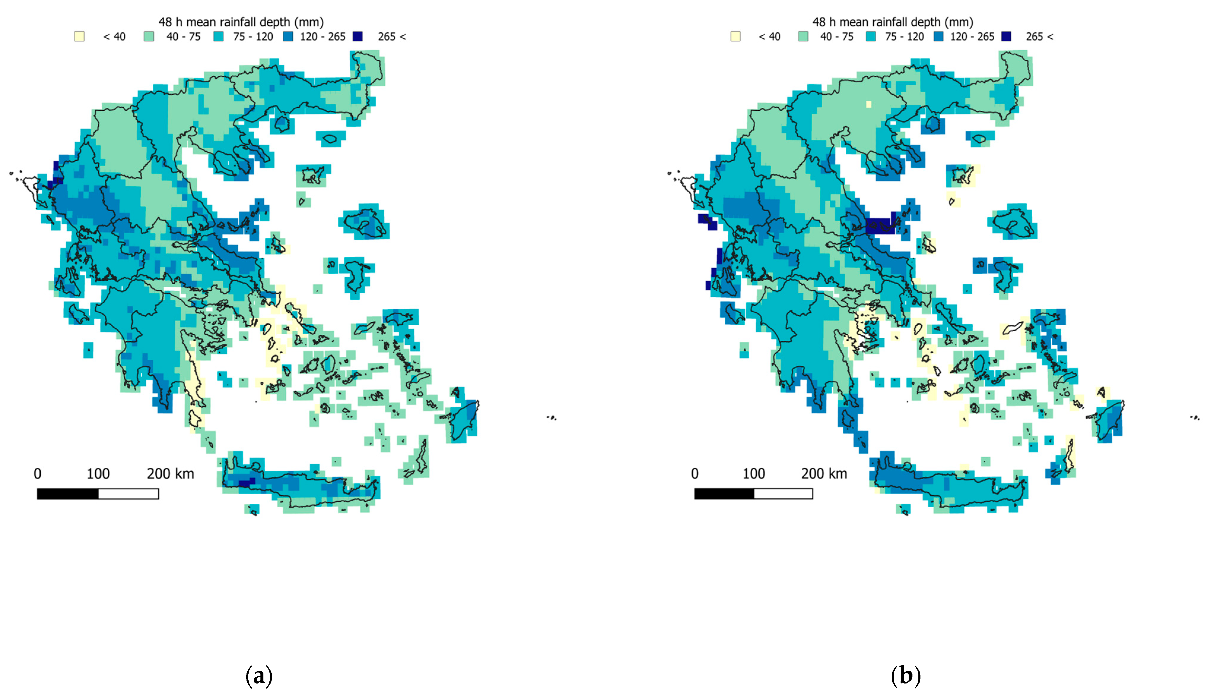
4.2. Regionalization of Average Maximum Rainfall for Different Scales
4.3. Assessment of Credible Intervals
4.4. Effect of Elevation on Multi-Scale Rainfall Patterns
5. Conclusions
Author Contributions
Funding
Data Availability Statement
Acknowledgments
Conflicts of Interest
References
- Claps, P.; Ganora, D.; Mazzoglio, P. Rainfall regionalization techniques. In Rainfall; Elsevier: Amsterdam, The Netherlands, 2022; pp. 327–350. [Google Scholar]
- Iliopoulou, T.; Malamos, N.; Koutsoyiannis, D. Regional ombrian curves: Design rainfall estimation for a spatially diverse rainfall regime. Hydrology 2022, 9, 67. [Google Scholar] [CrossRef]
- Zhang, Q.; Qi, T.; Singh, V.P.; Chen, Y.D.; Xiao, M. Regional frequency analysis of droughts in China: A multivariate perspective. Water Resour. Manag. 2015, 29, 1767–1787. [Google Scholar] [CrossRef]
- Zhao, L.; Liu, M.; Song, Z.; Wang, S.; Zhao, Z.; Zuo, S. Regional-scale modeling of rainfall-induced landslides under random rainfall patterns. Environ. Model. Softw. 2022, 155, 105454. [Google Scholar] [CrossRef]
- Crosta, G. Regionalization of rainfall thresholds: An aid to landslide hazard evaluation. Environ. Geol. 1998, 35, 131–145. [Google Scholar] [CrossRef]
- Sun, Q.; Miao, C.; Duan, Q.; Ashouri, H.; Sorooshian, S.; Hsu, K.L. A review of global precipitation data sets: Data sources, estimation, and intercomparisons. Rev. Geophys. 2018, 56, 79–107. [Google Scholar] [CrossRef]
- Huffman, G.J.; Stocker, E.F.; Bolvin, D.T.; Nelkin, E.J.; Tan, J. GPM IMERG Final Precipitation L3 Half Hourly 0.1 Degree x 0.1 Degree V06. Greenbelt 2019, MD: Goddard Earth Sciences Data and Information Services Center (GES DISC). Available online: https://gpm.nasa.gov/data/imerg (accessed on 8 November 2024).
- Hersbach, H.; Bell, B.; Berrisford, P.; Hirahara, S.; Horányi, A.; Muñoz-Sabater, J.; Nicolas, J.; Peubey, C.; Radu, R.; Schepers, D.; et al. The ERA5 global reanalysis. Q. J. R. Meteorol. Soc. 2020, 146, 1999–2049. [Google Scholar] [CrossRef]
- Saltikoff, E.; Friedrich, K.; Soderholm, J.; Lengfeld, K.; Nelson, B.; Becker, A.; Hollmann, R.; Urban, B.; Heistermann, M.; Tassone, C. An overview of using weather radar for climatological studies: Successes, challenges, and potential. Bull. Am. Meteorol. Soc. 2019, 100, 1739–1752. [Google Scholar] [CrossRef]
- Iliopoulou, T.; Koutsoyiannis, D. Have Rainfall Patterns Changed? A Global Analysis of Long-Term Rainfall Records and Re-Analysis Data; 47 pages, SR 306; The Heritage Foundation: Washington, DC, USA, 2025. [Google Scholar]
- Alfieri, L.; Avanzi, F.; Delogu, F.; Gabellani, S.; Bruno, G.; Campo, L.; Libertino, A.; Massari, C.; Tarpanelli, A.; Rains, D.; et al. High resolution satellite products improve hydrological modeling in northern Italy. Hydrol. Earth Syst. Sci. 2021, 2021, 1–29. [Google Scholar] [CrossRef]
- Thomopoulou, V.; Iliopoulou, T.; Kossieris, P.; Bariamis, G.; Tsoukalas, I.; Efstratiadis, A.; Makropoulos, C. A com-prehensive approach to building a continuous hydrologic model with Soil Moisture Accounting using Earth Observation data. Hydrol. Res. 2024, 55, 1161–1181. [Google Scholar] [CrossRef]
- Gebrechorkos, S.H.; Leyland, J.; Dadson, S.J.; Cohen, S.; Slater, L.; Wortmann, M.; Ashworth, P.J.; Bennett, G.L.; Boothroyd, R.; Cloke, H.; et al. Global scale evaluation of precipitation datasets for hydrological modelling. Hydrol. Earth Syst. Sci. 2023, 2023, 1–33. [Google Scholar] [CrossRef]
- Yonaba, R.; Belemtougri, A.; Fowé, T.; Mounirou, L.A.; Nkiaka, E.; Dembélé, M.; Komlavi, A.; Coly, S.M.; Koïta, M.; Karambiri, H. Rainfall Estimation in the West African Sahel: Comparison and Cross-Validation of Top-down vs. Bottom-up Precipitation Products in Burkina Faso. Geocarto Int. 2024, 39, 2391956. [Google Scholar] [CrossRef]
- Caloiero, T.; Pellicone, G.; Modica, G.; Guagliardi, I. Comparative analysis of different spatial interpolation methods applied to monthly rainfall as support for landscape management. Appl. Sci. 2021, 11, 9566. [Google Scholar] [CrossRef]
- Ahrens, B. Distance in spatial interpolation of daily rain gauge data. Hydrol. Earth Syst. Sci. 2006, 10, 197–208. [Google Scholar] [CrossRef]
- Zhang, W.; Liu, D.; Zheng, S.; Liu, S.; Loáiciga, H.A.; Li, W. Regional precipitation model based on geographically and temporally weighted regression kriging. Remote Sens. 2020, 12, 2547. [Google Scholar] [CrossRef]
- Malamos, N.; Koutsoyiannis, D. Bilinear surface smoothing for spatial interpolation with optional incorporation of an explanatory variable. Part 1: Theory. Hydrol. Sci. J. 2016, 61, 519–526. [Google Scholar] [CrossRef]
- Malamos, N.; Koutsoyiannis, D. Bilinear surface smoothing for spatial interpolation with optional incorporation of an explanatory variable. Part 2: Application to synthesized and rainfall data. Hydrol. Sci. J. 2016, 61, 527–540. [Google Scholar] [CrossRef]
- Pagliero, L.; Bouraoui, F.; Diels, J.; Willems, P.; McIntyre, N. Investigating regionalization techniques for large-scale hydrological modelling. J. Hydrol. 2019, 570, 220–235. [Google Scholar] [CrossRef]
- Ulrich, J.; Jurado, O.E.; Peter, M.; Scheibel, M.; Rust, H.W. Estimating IDF curves consistently over durations with spatial covariates. Water 2020, 12, 3119. [Google Scholar] [CrossRef]
- Mazzoglio, P.; Butera, I.; Claps, P. A local regression approach to analyze the orographic effect on the spatial variability of sub-daily rainfall annual maxima. Geomat. Nat. Hazards Risk 2023, 14. [Google Scholar] [CrossRef]
- Asong, Z.E.; Khaliq, M.N.; Wheater, H.S. Regionalization of precipitation characteristics in the Canadian Prairie Provinces using large-scale atmospheric covariates and geophysical attributes. Stoch. Environ. Res. Risk Assess. 2015, 29, 875–892. [Google Scholar] [CrossRef]
- Goovaerts, P. Geostatistical approaches for incorporating elevation into the spatial interpolation of rainfall. J. Hydrol. 2000, 228, 113–129. [Google Scholar] [CrossRef]
- Iliopoulou, T.; Koutsoyiannis, D.; Malamos, N.; Koukouvinos, A.; Dimitriadis, P.; Mamassis, N.; Tepetidis, N.; Markantonis, D. A stochastic framework for rainfall intensity–time scale–return period relationships. Part ΙΙ: Point modelling and regionalization over Greece. Hydrol. Sci. J. 2024, 69, 1092–1112. [Google Scholar] [CrossRef]
- Avanzi, F.; De Michele, C.; Gabriele, S.; Ghezzi, A.; Rosso, R. Orographic signature on extreme precipitation of short durations. J. Hydrometeorol. 2015, 16, 278–294. [Google Scholar] [CrossRef]
- Mazzoglio, P.; Butera, I.; Alvioli, M.; Claps, P. The role of morphology in the spatial distribution of short-duration rainfall extremes in Italy. Hydrol. Earth Syst. Sci. 2022, 26, 1659–1672. [Google Scholar] [CrossRef]
- Formetta, G.; Marra, F.; Dallan, E.; Zaramella, M.; Borga, M. Differential orographic impact on sub-hourly, hourly, and daily extreme precipitation. Adv. Water Resour. 2022, 159, 104085. [Google Scholar] [CrossRef]
- Marra, F.; Nikolopoulos, E.I.; Anagnostou, E.N.; Bárdossy, A.; Morin, E. Precipitation frequency analysis from remotely sensed datasets: A focused review. J. Hydrol. 2019, 574, 699–705. [Google Scholar] [CrossRef]
- Zhou, Y.; Matyas, C.J. Regionalization of precipitation associated with tropical cyclones using spatial metrics and satellite precipitation. GISci. Remote Sens. 2021, 58, 542–561. [Google Scholar] [CrossRef]
- Koutsoyiannis, D.; Iliopoulou, T.; Koukouvinos, A.; Malamos, N.; Mamassis, N.; Dimitriadis, P.; Tepetidis, N.; Markantonis, D. In search of climate crisis in Greece using hydrological data: 404 not found. Water 2023, 15, 1711. [Google Scholar] [CrossRef]
- Jarvis, A.; Reuter, H.I.; Nelson, A.; Guevara, E. Hole-Filled SRTM for the Globe Version 4, Available from the CGIAR-CSI SRTM 90m Database. 2008. Available online: http://srtm.csi.cgiar.org (accessed on 20 January 2023).
- Dalrymple, T. Flood-Frequency Analyses (No. 1543); US Government Printing Office: Washington, DC, USA, 1960. [Google Scholar]
- Malamos, N.; Koutsoyiannis, D. Field survey and modelling of irrigation water quality indices in a Mediterranean island catchment: A comparison between spatial interpolation methods. Hydrol. Sci. J. 2018, 63, 1447–1467. [Google Scholar] [CrossRef]
- Wahba, G.; Wendelberger, J. Some new mathematical methods for variational objective analysis using splines and cross validation. Mon. Weather. Rev. 1980, 108, 1122–1143. [Google Scholar] [CrossRef]
- Wahba, G. Bayesian “confidence intervals” for the cross-validated smoothing spline. J. R. Stat. Soc. Ser. B (Methodol.) 1983, 45, 133–150. [Google Scholar] [CrossRef]
- Dimitriadou, S.; Nikolakopoulos, K.G. Development of the Statistical Errors Raster Toolbox with Six Automated Models for Raster Analysis in GIS Environments. Remote Sens. 2022, 14, 5446. [Google Scholar] [CrossRef]
- Li, J.; Heap, A.D. A Review of Spatial Interpolation Methods for Environmental Scientists; Geoscience Australia: Canberra, Australia, 2008. [Google Scholar]
- Burrough, P.A.; McDonnell, R.A.; Lloyd, C.D. Principles of Geographical Information Systems; Oxford University Press: Oxford, UK, 2015. [Google Scholar]
- Beck, H.E.; McVicar, T.R.; Vergopolan, N.; Berg, A.; Lutsko, N.J.; Dufour, A.; Zeng, Z.; Jiang, X.; Van Dijk, A.I.J.M.; Miralles, D.G. High-Resolution (1 Km) Köppen-Geiger Maps for 1901–2099 Based on Constrained CMIP6 Projections. Sci. Data 2023, 10, 724. [Google Scholar] [CrossRef] [PubMed]
- Kazamias, A.P.; Sapountzis, M.; Lagouvardos, K. Evaluation of GPM-IMERG rainfall estimates at multiple temporal and spatial scales over Greece. Atmos. Res. 2022, 269, 106014. [Google Scholar] [CrossRef]
- Pradhan, R.K.; Markonis, Y.; Godoy, M.R.V.; Villalba-Pradas, A.; Andreadis, K.M.; Nikolopoulos, E.I.; Papalexiou, S.M.; Rahim, A.; Tapiador, F.J.; Hanel, M. Review of GPM IMERG performance: A global perspective. Remote Sens. Environ. 2022, 268, 112754. [Google Scholar] [CrossRef]


| Daily Rain Gauges | Sub-Daily Rain Recorders | ||||||||||||
|---|---|---|---|---|---|---|---|---|---|---|---|---|---|
| Timescale | 1 d | 2 d | 5 min | 10 min | 15 min | 30 min | 1 h | 2 h | 3 h | 6 h | 12 h | 24 h | 48 h |
| Number | 503 | 490 | 38 | 128 | 47 | 231 | 273 | 279 | 269 | 280 | 280 | 280 | 223 |
| Timescale | Number of Segments, mx | Number of Segments, my | τλx | τλy | τμx | τμy |
|---|---|---|---|---|---|---|
| 0.5 h | 9 | 140 | 0.884742 | 0.024031 | 0.001 | 0.001 |
| 1 h | 9 | 198 | 0.016242 | 0.009531 | 0.001 | 0.001 |
| 3 h | 9 | 254 | 0.001 | 0.001 | 0.001 | 0.001 |
| 6 h | 9 | 348 | 0.001 | 0.001 | 0.001 | 0.001 |
| 12 h | 9 | 448 | 0.001 | 0.001 | 0.001 | 0.001 |
| 24 h | 14 | 981 | 0.001 | 0.001 | 0.001 | 0.001 |
| 48 h | 14 | 387 | 0.001 | 0.001 | 0.001 | 0.001 |
| Daily Average | 6 | 147 | 0.99 | 0.001 | 0.652857 | 0.018715 |
| Surface Statistics (All Data) | Elevation | IMERG |
|---|---|---|
| MBE (mm) | 0.00 | 0.00 |
| MAE (mm) | 0.22 | 0.36 |
| RMSE (mm) | 0.31 | 0.49 |
| NSE | 0.90 | 0.74 |
| r2 | 0.90 | 0.74 |
| NRMSE (%) | 6.95 | 10.99 |
| σ (mm) | 0.89 | 0.83 |
| Surface Statistics (LOOCV) | Elevation | IMERG |
|---|---|---|
| MBE (mm) | −0.01 | 0.00 |
| MAE (mm) | 0.36 | 0.41 |
| RMSE (mm) | 0.49 | 0.55 |
| NSE | 0.74 | 0.67 |
| r2 | 0.75 | 0.67 |
| NRMSE (%) | 10.99 | 12.43 |
| Surface Statistics (All Data) | 0.5 h | 1 h | 3 h | 6 h | 12 h | 24 h | 48 h |
|---|---|---|---|---|---|---|---|
| Elevation | |||||||
| MBE (mm) | 0.00 | 0.00 | 0.00 | 0.00 | −0.01 | −0.01 | 0.00 |
| MAE (mm) | 2.75 | 3.18 | 4.01 | 5.36 | 6.95 | 7.27 | 9.01 |
| RMSE (mm) | 3.46 | 4.11 | 5.37 | 7.12 | 9.13 | 10.09 | 13.91 |
| NSE | 0.49 | 0.54 | 0.67 | 0.71 | 0.76 | 0.80 | 0.91 |
| r2 | 0.50 | 0.55 | 0.67 | 0.71 | 0.77 | 0.80 | 0.91 |
| NRMSE (%) | 13.08 | 12.68 | 8.63 | 8.10 | 6.78 | 5.23 | 5.50 |
| σ (mm) | 3.05 | 4.04 | 7.21 | 10.35 | 15.49 | 19.34 | 24.92 |
| IMERG | |||||||
| MBE (mm) | 0.00 | 0.00 | 0.00 | −0.01 | 0.00 | 0.00 | 0.00 |
| MAE (mm) | 2.99 | 3.50 | 4.18 | 4.57 | 7.56 | 9.33 | 10.58 |
| RMSE (mm) | 3.79 | 4.57 | 5.66 | 6.58 | 10.77 | 13.07 | 15.13 |
| NSE | 0.39 | 0.43 | 0.63 | 0.75 | 0.67 | 0.66 | 0.75 |
| r2 | 0.39 | 0.43 | 0.64 | 0.75 | 0.67 | 0.67 | 0.75 |
| NRMSE (%) | 14.34 | 14.12 | 9.10 | 7.49 | 7.99 | 6.78 | 5.98 |
| σ (mm) | 2.74 | 3.61 | 6.94 | 10.60 | 14.33 | 17.10 | 24.75 |
| Surface Statistics (LOOCV) | 0.5 h | 1 h | 3 h | 6 h | 12 h | 24 h | 48 h |
|---|---|---|---|---|---|---|---|
| Elevation | |||||||
| MBE (mm) | 0.05 | −0.42 | −1.84 | 0.15 | 1.61 | −0.17 | 0.21 |
| MAE (mm) | 3.51 | 4.51 | 13.54 | 8.20 | 12.77 | 11.25 | 11.52 |
| RMSE (mm) | 4.48 | 9.15 | 91.65 | 11.52 | 31.01 | 16.23 | 17.65 |
| NSE | 0.14 | −1.28 | −94.99 | 0.23 | −1.73 | 0.48 | 0.86 |
| r2 | 0.20 | 0.03 | 0.03 | 0.32 | 0.14 | 0.51 | 0.86 |
| NRMSE (%) | 16.94 | 28.23 | 147.34 | 13.10 | 23.01 | 8.42 | 6.98 |
| IMERG | |||||||
| MBE (mm) | −0.04 | −0.14 | −1.48 | −0.22 | −0.61 | −3.30 | −1.12 |
| MAE (mm) | 3.47 | 4.07 | 12.31 | 9.48 | 12.90 | 16.37 | 16.78 |
| RMSE (mm) | 4.46 | 5.38 | 78.04 | 16.47 | 24.35 | 79.25 | 28.13 |
| NSE | 0.15 | 0.21 | −68.60 | −0.57 | −0.68 | −11.42 | 0.13 |
| r2 | 0.18 | 0.23 | 0.03 | 0.16 | 0.11 | 0.04 | 0.33 |
| NRMSE (%) | 16.85 | 16.59 | 125.46 | 18.75 | 18.07 | 41.11 | 11.12 |
Disclaimer/Publisher’s Note: The statements, opinions and data contained in all publications are solely those of the individual author(s) and contributor(s) and not of MDPI and/or the editor(s). MDPI and/or the editor(s) disclaim responsibility for any injury to people or property resulting from any ideas, methods, instructions or products referred to in the content. |
© 2025 by the authors. Licensee MDPI, Basel, Switzerland. This article is an open access article distributed under the terms and conditions of the Creative Commons Attribution (CC BY) license (https://creativecommons.org/licenses/by/4.0/).
Share and Cite
Malamos, N.; Iliopoulou, T.; Dimitriadis, P.; Koutsoyiannis, D. Comparative Analysis of IMERG Satellite Rainfall and Elevation as Covariates for Regionalizing Average and Extreme Rainfall Patterns in Greece by Means of Bilinear Surface Smoothing. Geosciences 2025, 15, 212. https://doi.org/10.3390/geosciences15060212
Malamos N, Iliopoulou T, Dimitriadis P, Koutsoyiannis D. Comparative Analysis of IMERG Satellite Rainfall and Elevation as Covariates for Regionalizing Average and Extreme Rainfall Patterns in Greece by Means of Bilinear Surface Smoothing. Geosciences. 2025; 15(6):212. https://doi.org/10.3390/geosciences15060212
Chicago/Turabian StyleMalamos, Nikolaos, Theano Iliopoulou, Panayiotis Dimitriadis, and Demetris Koutsoyiannis. 2025. "Comparative Analysis of IMERG Satellite Rainfall and Elevation as Covariates for Regionalizing Average and Extreme Rainfall Patterns in Greece by Means of Bilinear Surface Smoothing" Geosciences 15, no. 6: 212. https://doi.org/10.3390/geosciences15060212
APA StyleMalamos, N., Iliopoulou, T., Dimitriadis, P., & Koutsoyiannis, D. (2025). Comparative Analysis of IMERG Satellite Rainfall and Elevation as Covariates for Regionalizing Average and Extreme Rainfall Patterns in Greece by Means of Bilinear Surface Smoothing. Geosciences, 15(6), 212. https://doi.org/10.3390/geosciences15060212