Iterative Inversion of Normal and Lateral Resistivity Logs in Thin-Bedded Rock Formations of the Polish Carpathians

Abstract

This study investigates the challenges and opportunities associated with improving the vertical resolution of normal and lateral resistivity logs in thin-bedded rock formations. The proposed iterative inversion procedure combines a finite element method forward modeling procedure with a particle swarm optimization algorithm to generate high-resolution models of the rock formation. The performance of the inversion approach was evaluated using synthetic datasets, and the results of the inversion of field data from thin-bedded formations of the Polish Carpathians are presented. This research highlights the potential of modern computational techniques to enhance the utility of historical resistivity logging data in current studies.

1. Introduction

The resistivity of rock formation is a crucial parameter measured during well logging. It is widely used in hydrocarbon exploration, groundwater studies, geotechnical engineering, and environmental surveys.

Normal and lateral tools belong to the family of multielectrode resistivity logging tools and are among the oldest logging tools to have been developed. Those tools were widely used in hydrocarbon exploration until the 1960s in the West and the 1990s in Eastern Bloc countries and still remain valuable for hydrogeological, geotechnical, and environmental surveys. Consequently, numerous boreholes exist where normal and lateral logs represent the primary or sole source of the formation resistivity data. These datasets are a unique and valuable resource that can contribute to ongoing and future prospection and research. However, due to the extremely simple construction and lack of any focusing of electric current, the resolution of the resistivity logs obtained using normal and lateral tools is inferior to those generated by modern and more advanced logging tools. In addition, lateral tools produce non-symmetric logs, which add another layer of challenges to the interpretation procedure [1,2,3,4,5,6,7,8]. Detailed information about the history, configurations, measurement, and interpretation principles of normal and lateral tools can be found in the referenced publications [8,9,10,11,12,13].

The inversion of normal and lateral resistivity logs has been studied in the past by numerous authors. The process initially relied on analytical solutions for horizontally layered media without the consideration of borehole effects, where model parameters were manually adjusted by the interpreter to fit observations [14]. This modeling approach was later paired with a ridge regression algorithm to perform the iterative inversion of normal and lateral logs [15]. The introduction of axisymmetric finite difference methods enabled more accurate forward modeling by accounting for borehole effects and more complex formation geometries [16,17,18]. This was further improved by adopting axisymmetric finite element methods, allowing for greater flexibility in model geometry [19,20]. To reduce computational demands, rapid inversion methods were developed, combining 1D and 2D inversion schemes into efficient iterative procedures [21,22]. More recent studies have integrated axisymmetric finite element modeling with conjugate gradient optimization to jointly invert short- and long-normal logs, producing blurred images of resistivity variations around the borehole and enabling the recovery of structural information from resistivity logs [23,24]. However, because advancements in well logging are primarily driven by the hydrocarbon exploration industry, and significant developments in computational technology have occurred after the widespread use of normal and lateral tools in hydrocarbon exploration has declined in Western countries, research efforts have predominantly focused on more modern resistivity logging tools [3,25].

This study explores the opportunities and challenges associated with enhancing the vertical resolution of normal and lateral resistivity logs recorded in thin-bedded rock formations in the Polish Carpathians using an iterative inversion procedure.

The sandy–shaly formations in the Polish Carpathians present unique challenges for well-logging applications. These formations are characterized by thinly bedded sequences of sandstones, mudstones, shales, and heteroliths, often with individual layers thinner than the vertical resolution of the logging tools. This thin-bedded nature leads to the averaging of log responses, potentially obscuring the true properties of the rock formation.

Two approaches have been developed to improve the accuracy of well log interpretation in thin-bedded rock formations. High-resolution methods involve constructing a detailed, deterministic formation model with estimated properties for each individual bed, whereas low-resolution methods entail developing a statistical formation model that describes the composite properties of the thin-bedded interval [26].

Over the years, several authors have addressed the problem of increasing the accuracy of formation evaluation in sandy–shaly formations in the Polish Carpathians by employing both high-resolution and low-resolution methods [27,28,29,30,31,32,33,34]. Studies aimed at enhancing the vertical resolution of resistivity logs have predominantly focused on induction logging tools, which are characterized by significantly greater vertical resolution than normal and lateral resistivity logs.

The iterative inversion algorithm described in this paper employs the finite element method (FEM) to generate synthetic resistivity logs and utilizes the particle swarm optimization (PSO), a population-based global optimization algorithm, to identify optimal solutions. The accuracy of the inversion results was evaluated through synthetic data tests, and the inversion results from field data from the Polish Carpathians are also presented.

2. Materials and Methods

2.1. Normal and Lateral Resistivity Logs

Normal and lateral logging tools comprise two circuits: a current circuit and a measurement circuit. Conventionally, the current electrodes are designated as A and B, while the potential electrodes are labelled as M and N. Three electrodes are positioned in close proximity, with the fourth electrode located at an effective infinity. In a normal configuration, the two nearest electrodes belong to different circuits, the response of the tool is symmetric, and electrode spacing is defined as the distance between these adjacent electrodes. Conversely, in a lateral configuration, the two closest electrodes are part of the same circuit, the response of the tool is non-symmetric, and the tool spacing is determined by the distance between the measurement point and the furthest of the three downhole electrodes. Generally, increasing the electrode spacing enhances the depth of investigation while diminishing the vertical resolution; thus, logging tools with larger electrode spacing are less influenced by borehole and mud filtration and more affected by adjacent beds than logging tools with smaller electrode spacing [8,12,35].

Typically, normal and lateral logging tools are deployed in sets consisting of several tools with varying electrode spacings to derive the radial resistivity profile of the rock formation around the borehole. The set of resistivity logs analyzed in this study is commonly used in boreholes from the area of the Polish Carpathians. It comprises two normal and two lateral resistivity tools with varying radial depths of investigation: E16N (A0.4M6.0N), E64N (A1.62M6.0N), EL14 (A4.0M0.5N), and EL28 (A8.0M1.0N). The E16N logging tool (short-normal tool) investigates a shallow radial depth, primarily assessing the invaded zone near the borehole. In contrast, the E64N (long-normal tool) probes deeper into the formation, often reaching beyond the invaded zone to provide some information about the uninvaded formation. Meanwhile, the EL14 and EL28 (lateral tools) are intended to measure the resistivity at greater radial depths, thereby providing a clearer picture of the properties of the uninvaded formation.

2.2. Inversion Procedure

2.2.1. Iterative Inversion

The iterative inversion method is widely employed in well-logging applications. Unlike approaches that attempt to reverse the physical processes occurring during well logging, this method relies on iterative forward modeling to identify a formation model that best fits the observed data. The process begins with the creation of an initial formation model. Based on this model, a synthetic log is generated and compared to the measured log. If the difference between the two is sufficiently small, the model is accepted as the solution. Otherwise, the formation model is adjusted and the synthetic log is recalculated and compared again with the measured data. This cycle is repeated until the synthetic and measured logs achieve an acceptable level of agreement. The specific design of the iterative inversion algorithm is largely determined by the formulation of the forward problem and the method used to optimize the solution. Model parameters can be adjusted manually by the analyst to achieve a satisfactory fit, either qualitatively or quantitatively; however, more commonly, local or global optimization techniques are applied to minimize the objective function, which quantitatively measures the difference between synthetic and observed data [26,32,36].

2.2.2. Formation Model

The model considered in this study comprises the borehole and formation layers that are perpendicular to the borehole axis and are characterized by a single parameter whose value corresponds to the value of the logging tool measurement in an infinitely thick layer with the same properties.

Since the vast majority of commonly used optimization algorithms (including the algorithm used in this study) do not allow for changes in the number of model parameters (e.g., adding or removing layers from the model) during the optimization process, it is necessary to establish the model’s geometry before the start of the optimization procedure. In this study, the rock formation is approximated as a sequence of equally thick layers with boundaries located halfway between measurement points [37]. The model parameters under optimization are the resistivities of the individual layers that build the model:

$$\mathit{x}=\left[x_1,x_2,x_3,\dots ,x_n\right],$$

(1)

where $x_1,x_2,x_3, \dots , x_n$ are the parameters of the layers and $n$ is the number of layers in the model. Other parameters, such as borehole geometry, mud resistivity, and locations of layer boundaries, are assumed to be known and remain constant during the optimization procedure.

2.2.3. Forward Modeling

The modeling code used to generate the results shown in this study is based on ReMo3D, an open-source finite element method modeling toolkit for normal and lateral resistivity logs in Python [8].

In this framework, logging tools are represented as point electrodes in a two-dimensional, axisymmetric domain. The simulation domain is centered on a single current electrode or the midpoint between the two current electrodes depending on the tool configuration. Along the borehole axis, a Neumann boundary condition is imposed to ensure symmetry, whereas external boundaries are treated with a Dirichlet boundary condition. The forward problem is solved using the finite element method. The value of the electric potential at the location of the measuring electrodes is retrieved from the model and used to calculate the value of the measured apparent resistivity assigned to the depth at which the measurement point of the tool is located [8].

2.2.4. Optimization Procedure

The optimization code used to generate the results shown in this paper is based on PySwarms, an open-source research toolkit for particle swarm optimization in Python [38].

The particle swarm optimization is a population-based stochastic optimization algorithm inspired by the behavior of bird flocks searching for food sources. It belongs to the class of global optimization methods and was proposed and initially developed by Kennedy and Eberhart [39,40]. Over the years, many variants, enhancements, and extensions of the original version of the algorithm have been proposed. The version of the algorithm utilized in this study is based on the original work by Kennedy, Eberhart, and Shi and is commonly referred to as standard particle swarm optimization (SPSO) [39,40,41,42,43,44].

The PSO algorithm maintains a swarm of particles, where each particle represents a potential solution to the optimization problem. A swarm of particles traverses a multidimensional search space by iteratively updating its velocity and position based on both individual experiences and the social interactions between particles. Specifically, each particle maintains a record of its personal best position ${\mathit{y}}_i$ and is simultaneously influenced by the global best position $\widehat{\mathit{y}}$ found by the swarm. The dynamics of each particle are governed by a velocity update rule that integrates three components: an inertia term, a cognitive term, and a social term [42,43,44]:

$${\mathit{v}}_i\left(t+1\right)={w{·\mathit{v}}_i\left(t\right)+c}_1{\mathit{r}}_1\left(t\right)\left[{\mathit{y}}_i\left(t\right)-{\mathit{x}}_i\left(t\right)\right]+c_2{\mathit{r}}_2\left(t\right)\left[\widehat{\mathit{y}}\left(t\right)-{\mathit{x}}_i\left(t\right)\right]$$

(2)

where ${\mathit{v}}_i\left(t\right)$ and ${\mathit{x}}_i\left(t\right)$ represent the velocity and position of particle $i$ at iteration $t$, respectively; $w$ is the inertia weight that moderates the influence of the velocity from the previous iteration; $c_1$ and $c_2$ are acceleration coefficients controlling the contributions of the cognitive and social components; and ${\mathit{r}}_1$ and ${\mathit{r}}_2$ are uniformly distributed random variables in the interval [0, 1] generated separately for each particle at each iteration, which introduces stochasticity into the search process. The values of the acceleration coefficients remain constant, whereas the value of the inertia weight gradually decreases during the optimization procedure. After updating the velocity, the particle’s position is revised according to the following rule [42,43,44]:

$${\mathit{x}}_i\left(t+1\right)={\mathit{x}}_i\left(t\right)+{\mathit{v}}_i\left(t+1\right).$$

(3)

This iterative process enables the swarm to balance the exploration of the search space with the exploitation of promising regions, thereby enhancing the probability of convergence to a near-optimal solution. The approach described above is called the global best particle swarm optimization algorithm (gbest PSO) because all particles are connected and the social component moves all particles to the same position: the best position discovered so far by the entire swarm [42,43,44].

2.2.5. Inversion Workflow

The iterative inversion algorithm used in this study integrates finite element forward modeling with particle swarm optimization to estimate the resistivity distribution of the rock formation. This section provides a step-by-step outline of the workflow, clarifying the interaction between the two computational components.

• Initialization:
  A swarm of particles is generated. Each particle represents a candidate resistivity model composed of resistivity values assigned to a fixed sequence of layers in the formation. These initial models are generated by randomly sampling resistivity values within predefined bounds, ensuring a diverse and representative starting point for the search.
• Forward Modeling:
  For each particle, a synthetic resistivity log is computed using a finite element method based on the formation model represented by that particle.
• Objective Function Evaluation:
  The synthetic logs generated for each particle are compared against the input resistivity data, and a misfit is computed using the root mean square error (RMSE) across all measurement points, quantifying the discrepancy between the synthetic and observed logs.
• Parameter Update:
  The swarm is updated by adjusting each particle’s velocity and position. These updates are based on the particle’s own best-known solution and the global best solution found so far by the swarm according to SPSO dynamics involving inertia, cognitive, and social components.
• Convergence Check:
  Steps 2 through 4 are repeated iteratively until a stopping criterion is met: either a predefined number of iterations is completed or the objective function reaches a predefined minimum threshold.

This structured interaction between FEM and PSO allows for efficient global optimization in a complex, multidimensional parameter space. The results presented later in this study were obtained by running a swarm of 50 particles over 1000 iterations. Computation time on a workstation equipped with an AMD Ryzen Threadripper 3960X CPU ranged from 8 to 10 h per example, with field cases taking slightly longer than synthetic ones due to the greater number of log measurement points (101 vs. 81). These runtimes reflect a known drawback of global optimization methods, which are more computationally demanding than local optimization approaches. However, each log response for each particle requires simulations at multiple measurement points, all of which are independent and can be executed in parallel given sufficient computing resources. As a result, the forward modeling step is highly parallelizable, offering near-linear speed-up with increasing thread count, up to a practical limit defined by the product of the number of particles and measurement points. This scalability enables substantial reductions in computation time when run on more powerful multi-core hardware or distributed computing environments.

2.3. Factors Affecting the Results of the Inversion Procedure

The accuracy of the results obtained in the inversion procedure depends on the quality of the input data, the performance of the optimization procedure, the proper modeling of physical processes, and correct assumptions about the parameters and conditions in the subsurface.

Incorrect assumptions about mud resistivity, misalignment in measurement depths, missing data, boundary effects present due to the nature of working on a finite depth interval, and incorrect assumptions about model geometry or insufficient model complexity can affect the results of inversion.

Other factors that can affect the result of inversion, such as not accounting for borehole trajectory, the dip of the layers in relation to the borehole axis, resistivity anisotropy, and the eccentricity of the tool in the borehole, will not be considered in this study due to the limitations of the utilized software.

2.3.1. Incorrect Mud Resistivity

Drilling mud resistivity directly affects the tool’s response, particularly in regions where the borehole effect is significant or in the case of shorter logging tools whose readings are more significantly affected by the borehole. If the mud resistivity is overestimated or underestimated, the calculated formation resistivity is systematically biased. The mud resistivity value in borehole conditions utilized during the interpretation procedure might be incorrect because of incorrect or insufficient information about the resistivity and/or the temperature of the mud sample or due to an incorrect or too simplistic model of changes in temperature with depth.

2.3.2. Misalignments in Measurement Depths

Depth misalignment between the depths to which measurements are assigned and the actual depth at which they were conducted can shift the resistivity responses and distort well logs. These errors might occur as a result of the measuring procedure or as a result of depth shifts applied to the data during the depth-matching procedure.

2.3.3. Boundary Effects

During the inversion of the well logs procedure, it is common practice to assume that the resistivity beyond the analyzed interval is constant. As a consequence of this assumption, boundary effects can occur, particularly if the resistivity varies significantly beyond the analyzed interval. This results in artefacts near the boundaries of the analyzed interval.

2.3.4. Assumptions About the Model

The model utilized in the inversion procedure is always a simplification of the real conditions under which a measurement was made. However, an oversimplified model (e.g., one that does not contain sufficiently thin layers) or a model with incorrect geometry (e.g., incorrect positions of layer boundaries) can fail to capture resistivity variations or destabilize the inversion procedure.

2.4. Data

2.4.1. Synthetic Data

Any of the factors described above in isolation can affect the results of the inversion procedure and lead to untrue and unrealistic results. When combined, the effects of these factors can become even more significant. To analyze these effects, the algorithm was tested on synthetic data (Figure 1 and Figure 2).

The models were prepared as follows. The formation was divided into major intervals of thicknesses that were multiples of the logging step (which, for that simulation, was set to 0.25 m) with the boundaries located precisely halfway between the depths of the measurement points. The locations of the interval boundaries were perturbed by adding to them a value randomly chosen from the uniform distribution in the interval [−0.125 m, 0.125 m]. Each major interval was further divided into smaller subintervals, with a thickness of approximately 0.125 m. The locations of the subinterval boundaries were perturbed by adding to them a value randomly chosen from the uniform distribution in the interval [−0.0625 m, 0.0625 m]. Resistivity values in the range of 1 to 10 Ωm were assigned to each of the major intervals, and the value of resistivity in each subinterval was randomly chosen from the normal distribution with a mean equal to the resistivity value assigned to the major interval to which that subdivision belongs and a standard deviation of 0.5 Ωm. The second variation of the model is identical to the first, except that the intervals at the top and bottom of the model were replaced by thick uniform layers to prevent the occurrence of boundary effects. Both models contained a borehole with a constant diameter of 0.2 m filled with drilling mud with a resistivity of 0.35 Ωm.

For each model, two sets of normal and lateral resistivity logs were generated, one where true measurement depths were aligned with depths to which measurements were assigned, and one where true measurement depths were misaligned with depths to which measurements were assigned, which resulted in four distinct sets of synthetic logs: logs unaffected by boundary effects and measurement depth misalignment, logs affected only by boundary effects, logs affected only by measurement depth misalignment, and logs affected by both boundary effects and measurement depth misalignment.

No additional stochastic noise was introduced into the synthetic logs. This decision was made deliberately, as the primary objective of the synthetic data tests was to isolate and examine the influence of specific factors that a log interpreter can actively manage or at least partially account for during the interpretation process. Excluding random noise ensured a controlled test environment in which the effects of each factor on the inversion outcome could be clearly attributed and interpreted without interference from unstructured variability. The inclusion of synthetic noise would have introduced an additional layer of complexity, potentially obscuring the individual contributions of these targeted parameters. The synthetic tests were, therefore, designed to assess the robustness of the inversion algorithm under idealized yet practically meaningful conditions, reflecting challenges commonly encountered in field applications and interpretation workflows.

2.4.2. Field Data

The algorithm was tested on data from a borehole located within the Eastern Carpathians, Poland, where normal and lateral resistivity logs were run in the same depth intervals as the relatively modern resistivity logging tool, the High Resolution Array Induction (HRAI) tool. The HRAI logs were acquired with a logging step of 0.1 m. Although normal and lateral logs were also available in the selected borehole with a 0.1 m logging step, data with a 0.25 m logging step were chosen for this study, as this step size is more commonly found in older boreholes, where normal and lateral logs often serve as the sole or primary source of formation resistivity information. This allowed the performance of the inversion algorithm to be assessed in real-life scenarios. The depth intervals selected for the test are located within the Ropianka Formation (Inoceramid Beds) of the Skole Unit. Lithologically, the intervals are dominated by silty–clayey shales. Compact mudstones and fine-grained calcareous sandstones are also present.

Two depth intervals were analyzed. The first interval (Figure 3) represents a simpler lithological structure, characterized by thicker beds and more gradual resistivity transitions. In contrast, the second interval (Figure 4) exhibits a more complex structure, with multiple thin beds, sharp resistivity contrasts, and finer-scale variability. These differences in geological complexity are expected to influence the performance of the inversion, with the second interval posing a greater challenge due to its fine layering, abrupt resistivity changes, and overall structural complexity.

One important consideration is that, unlike in the case of synthetic data, a direct comparison is not possible in this case. Due to differences in the physics of measurement between the electrode and induction logging tools, and the fact that the induction logging tool was run under suboptimal conditions (high mud conductivity), it measured lower resistivity values in comparison to electrode logging tools. Furthermore, the HRAI logs were acquired two days after the normal and lateral logs, which may have influenced certain properties of the logging environment (e.g., the development of mud cake as well as changes in flushed and filtration zones), potentially affecting the logging results.

3. Results

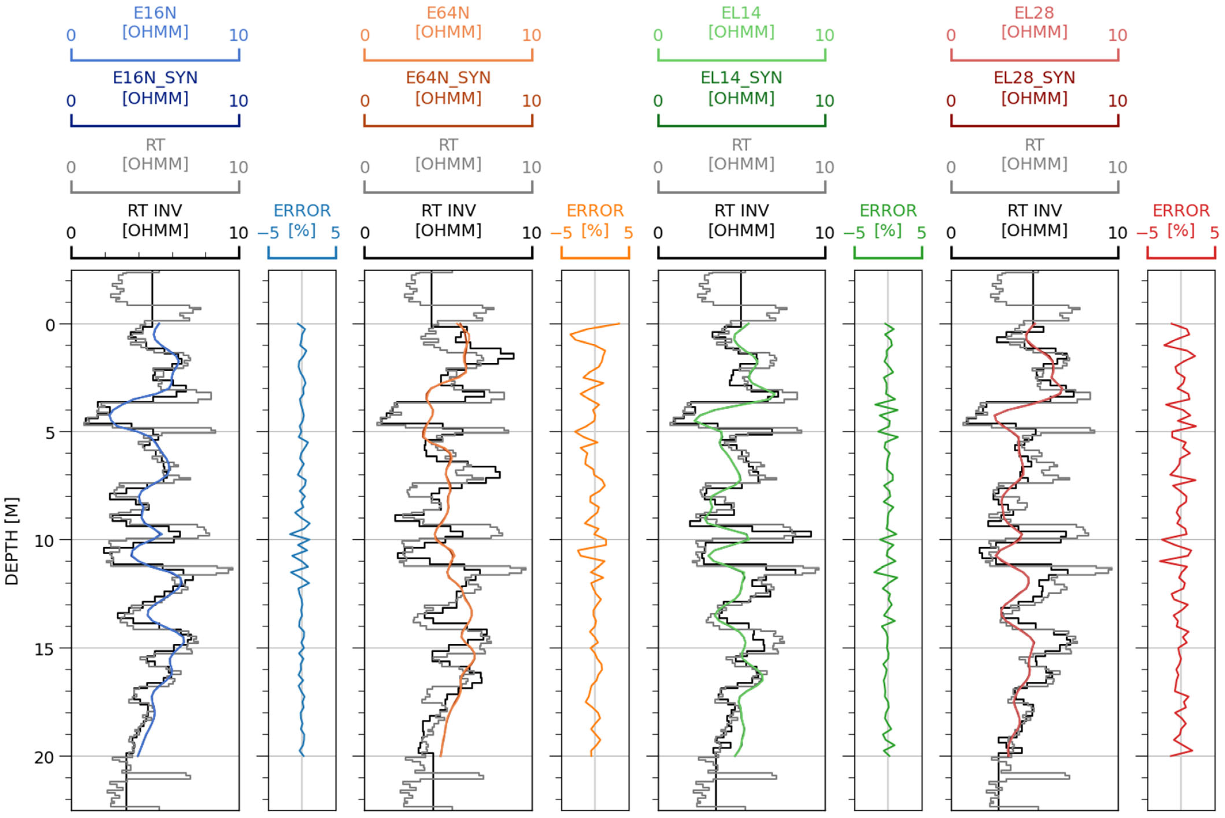
3.1. Results of Inversion of Synthetic Data

Each set of generated synthetic logs was inverted three times with the assumption that mud resistivity is equal to 0.20 Ωm, 0.35 Ωm, and 0.50 Ωm. When the assumed mud resistivity differs from the true value, the inversion results are further impacted by errors associated with incorrect mud resistivity, in addition to other factors affecting the logs. This resulted in a dataset of inversion results ranging from logs unaffected by any of the discussed factors to logs simultaneously affected by all three factors (incorrect mud resistivity, boundary effects, and incorrect measurement depths).

Due to the large volume of data, only two extreme examples are explicitly shown in this publication (Figure 5 and Figure 6). The complete dataset is presented in the form of scatter plots that display the relative model error versus relative log error, complemented by kernel density estimation (KDE) plots of each parameter distribution (Figure 7). The figure illustrates how different error sources—incorrect mud resistivity, boundary effects, and misaligned measurement depths—impact both the reconstructed formation resistivity (relative model error) and the agreement between synthetic and input well logs (relative log error). The distribution of data along the x-axis (relative model error) indicates how well the inversion results approximate the true variations in resistivity within the rock formation, whereas the distribution of data along the y-axis (relative log error) reflects the degree to which the generated synthetic data fit the actual well logs. To complement these qualitative patterns, Figure 8 provides a quantitative summary of inversion performance across all test cases using two error metrics: mean log RMSE and mean model RMSE, presented as heatmaps. The top panel shows the average discrepancy between the synthetic logs generated during inversion and the original input logs, while the bottom panel displays the deviation between the inverted formation models and the true synthetic models used to generate those input logs.

Across all tested cases, an interesting and somewhat counterintuitive trend emerges: the log RMSE consistently decreases as the assumed mud resistivity increases, even when the assumed value is higher than the true mud resistivity. In all scenarios, using a mud resistivity that is too high results in a better fit between synthetic and input logs than using the correct value. This behavior is observed regardless of the presence or absence of boundary effects and depth misalignments. This result may be counterintuitive at first glance but is likely rooted in the physics of electrode-based measurements. Increasing the assumed mud resistivity reduces the modeled conductivity of the borehole, forcing the synthetic tool response to rely more heavily on formation resistivity contrasts. As a result, synthetic logs become more formation-sensitive, which, in turn, improves their alignment with the input data. While this effect may enhance the fit of the logs (reducing log RMSE), it does not necessarily improve the reconstruction of the true resistivity model, as evidenced by the increase in model RMSE. This suggests that a higher-than-true mud resistivity may act as an implicit regularization mechanism, stabilizing inversion in the presence of other errors (e.g., boundary effects, depth misalignments), even though the assumption itself is incorrect.

When the mud resistivity assumed in the inversion does not correspond to the actual borehole conditions, the inversion compensates by adjusting the estimated formation resistivities. This adjustment introduces a systematic bias in the model values and degrades the agreement between synthetic and input well logs. The data exhibit increased log errors, characterized by broader distributions and deviations of synthetic logs from the input logs. Consequently, the scatter plots reveal that incorrect mud resistivity results in a wider or shifted distribution of the model error, highlighting the inversion’s challenge in reconciling discrepancies in borehole parameters.

In the absence of boundary effects, the inversion is constrained solely by the analyzed depth interval, leading to a more compact data cluster. This indicates that the inversion process can accurately capture resistivity variations without introducing artefacts from beyond the analyzed interval. However, when the resistivity of the formations outside the analyzed interval deviates significantly from the assumed constant value, edge artefacts emerge. These artefacts manifest as a broader spread in both the model and log errors, particularly near the interval boundaries. In the scatter plots, this appears as a wider distribution, illustrating the difficulties in fitting logs near the edges of the analyzed interval.

Accurate measurement depths allow for the inversion to correctly align log readings with their true subsurface positions, resulting in an improved agreement between synthetic and measured logs (lower vertical scatter) and more reliable formation resistivity estimates (narrower horizontal spread). In contrast, misaligned measurement depths shift resistivity readings relative to their actual positions, increasing log error (as indicated by greater vertical scatter) and potentially introducing systematic biases or increased variability in formation resistivity estimates.

Overall, the top row and center column of Figure 7 represent the idealized scenario (correct mud resistivity, correct measurement depths, and no boundary effects), with the smallest scatter in both the model and log errors. Departures from these ideal conditions, whether due to incorrect mud resistivity, boundary effects, or depth misalignments, result in broader and/or skewed distributions, shifting them away from zero. The RMSE heatmaps in Figure 8 further quantify these effects, confirming the relative importance of each factor and highlighting the complex ways in which inversion quality depends on data quality.

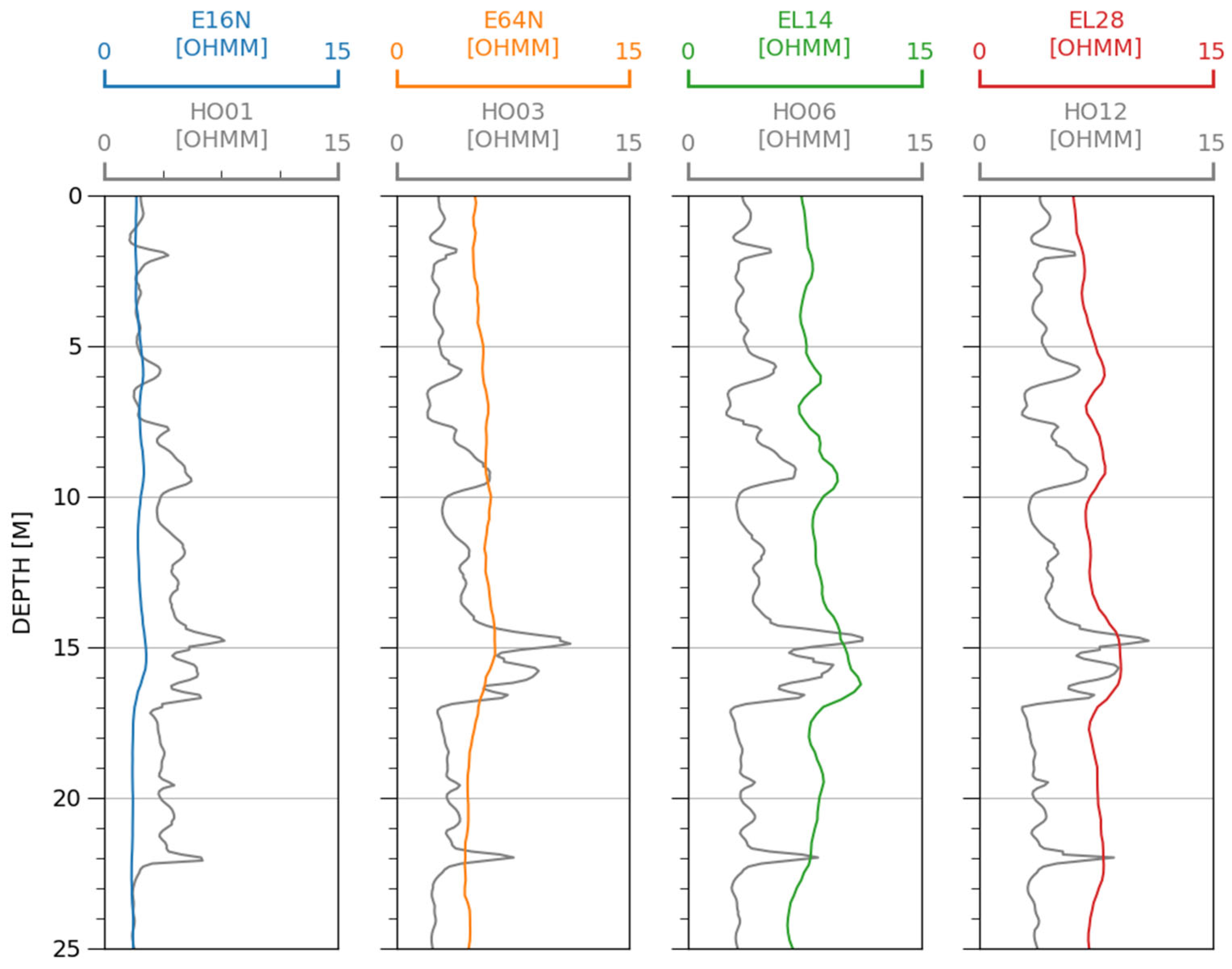
3.2. Results of the Inversion of Field Data

Figure 9 and Figure 10 present the inversion results for four legacy resistivity logs (E16N, E64N, EL14, and EL28) from a borehole in the Eastern Carpathians, Poland, along with relatively modern HRAI logs. The results from the two analyzed intervals are very similar and, therefore, will be discussed jointly, although notable differences related to the geological complexity of each interval are highlighted. An important consideration in these comparisons is that, as discussed earlier, a systematic difference in the measured resistivity values exists between the normal and lateral logging tools and the HRAI logging tool. Consequently, the evaluation of inversion quality is based on the qualitative assessment of the relative similarity of the observed patterns rather than the absolute resistivity values.

In the case of the E16N tool, its relatively close electrode spacing results in a very shallow depth of investigation, implying that the borehole and filtration zone effects strongly dominate the measured signal. Consequently, the inversion procedure introduced extremely limited improvements. The resulting resistivity distribution remains largely similar to the original E16N log, which, in turn, leads to only a minimal improvement in matching the trends that are visible on the HRAI log. Essentially, the inversion is constrained by the overwhelming influence of the borehole and near-borehole conditions captured by the E16N tool.

In contrast, the inversion results for the E64N and EL28 logs demonstrate more substantial improvements, particularly in the first, simpler interval. In this interval, the inversion for both tools achieved quite good (E64N) or good (EL28) improvements, successfully capturing the large-scale variations in the formation resistivity and delineating major bed boundaries present in the HRAI logs. Some finer resistivity variations were also reasonably resolved. However, in the second, more complex interval, the improvements for both E64N and EL28 were only moderate. While the inversion results still captured the broader trends, the finer-scale features and subtle resistivity contrasts were significantly less well resolved.

The inversion of the EL14 log consistently yielded the most favorable outcomes across both intervals. In the first interval, the resulting resistivity distribution closely follows trends observed on the HRAI log, effectively capturing both the broad resistivity variations and the finer-scale features and subtle resistivity contrasts. Even in the more challenging second interval, the EL14 inversion achieved good improvement, successfully reflecting major resistivity trends and reproducing many of the subtle resistivity contrasts visible in the high-resolution data.

A key observation from these results is that the synthetic logs generally follow the trends of the original field logs, indicating that the inversion procedure can replicate the measured data with reasonable accuracy. This is reinforced by the relatively small relative error values, which generally remain within the ±5% range. However, in the analyzed scenarios, the degree of improvement clearly depends on both the tool configuration and the geological complexity of the interval.

4. Discussion

This study demonstrates that modern computational techniques under favorable conditions can significantly enhance the vertical resolution and interpretability of legacy normal and lateral resistivity logs in thin-bedded rock formations, thereby extending the utility of historical logging data for detailed formation evaluation.

Synthetic data tests underscore the importance of careful data preparation in achieving reliable inversion outcomes. In particular, the use of accurate mud resistivity values, precise measurement depth alignment, and the careful selection of interval boundaries—avoiding placement near major resistivity contrasts—were identified as major factors affecting the quality of inversion results. Deviations from these conditions introduce systematic biases, as reflected by increased discrepancies between the formation models obtained through the inversion procedure and the true synthetic models.

The application of the inversion methodology to field data from the Eastern Carpathians, Poland, further demonstrates both the potential and the limitations of the approach. Tests performed on two depth intervals of varying structural complexity revealed varying levels of success across different logging tools. In the first, structurally simpler interval, the inversion procedure yielded significant improvements across most tools. The E64N and EL28 logs showed good alignment with HRAI trends, and the EL14 log delivered very good correspondence, capturing both large-scale resistivity variations and finer-scale contrasts. In the second, more complex interval, the performance varied more strongly. The EL14 tool continued to provide good inversion results, but the E64N and EL28 logs exhibited only moderate improvements, struggling to resolve fine layering and sharp transitions. The E16N tool, dominated by borehole effects, showed virtually no enhancement in both intervals. These results confirm that, while inversion improves legacy log quality in general, its effectiveness depends on the quality of the input data, the configuration of the logging tools, and the geological complexity of the formation.

The computation times observed in this study reflect a known drawback of global optimization methods, which are inherently more computationally demanding than local approaches. Each inversion run—for relatively short depth intervals—required several hours of computing. However, it should be noted that the workstation used in this study did not fully leverage the parallel nature of the forward modeling step. As a result, significant reductions in runtime are achievable by utilizing more powerful multi-core hardware or distributed computing environments. Practical implementations should take advantage of this parallelizability to improve scalability and make the method more efficient for larger datasets.

5. Conclusions

The iterative inversion procedure, based on finite element forward modeling and particle swarm optimization, demonstrated the potential to integrate historical logging data into contemporary studies. By enhancing the resolution of older datasets, the method enables a more comprehensive interpretation of thin-bedded formations, thus contributing to an improved formation evaluation in complex geological settings, such as the Polish Carpathians.

References

1. Keys, W.S. Borehole Geophysics as Applied to Groundwater. In Mining and Groundwater Geophysics/1967, Proceedings of the Canadian Centennial Conference on Mining and Groundwater Geophysics, Niagara Falls, ON, Canada, October 1967; Morley, L.W., Ed.; Economic Geology Report; Department of Energy, Mines, and Resources: Ottawa, ON, Canada, 1970. [Google Scholar]
2. Keys, W.S.; MacCary, L.M. Application of Borehole Geophysics to Water-Resources Investigations; U.S. G.P.O.: Washington, DC, USA, 1971. [Google Scholar]
3. Allaud, L.A.; Martin, M.H. Schlumberger: The History of a Technique; John Wiley & Sons: New York, NY, USA, 1977. [Google Scholar]
4. Keys, W.S. Borehole Geophysics Applied to Ground-Water Investigations; U.S. G.P.O: Washington, DC, USA, 1990. [Google Scholar]
5. International Atomic Energy Agency (IAEA). Characterization of Groundwater Flow for Near Surface Disposal Facilities; International Atomic Energy Agency: Vienna, Austria, 2001. [Google Scholar]
6. Asquith, G.; Krygowski, D. Basic Well Log Analysis, 2nd ed.; American Association of Petroleum Geologists: Tulsa, OK, USA, 2004; ISBN 978-0-89181-667-6. [Google Scholar]
7. Acworth, I. Investigating Groundwater; CRC Press: London, UK, 2019; ISBN 978-1-351-00852-5. [Google Scholar]
8. Wilkosz, M. ReMo3D—An Open-Source Python Package for 2D and 3D Simulation of Normal and Lateral Resistivity Logs. Geol. Geophys. Environ. 2022, 48, 195–211. [Google Scholar] [CrossRef]
9. Wiltgen, N.A. The Essential of Basic Russian Well Logs and Analysis Techniques. In Proceedings of the SPWLA 35th Annual Logging Symposium, Tulsa, OK, USA, 19–22 June 1994. [Google Scholar]
10. Wiltgen, N.A.; Truman, R.B. Russian Lateral (BKZ) Analysis. In Proceedings of the SPE Annual Technical Conference and Exhibition, Houston, TX, USA, 3–6 October 1993. [Google Scholar]
11. Jakubowicz, W. Russian Well Log Mnemonics. In Russian-Style Formation Evaluation; Harrison, B., Ed.; The London Petrophysical Society and The Geological Society of London: London, UK, 1995; pp. 211–220. [Google Scholar]
12. Vincent, M.; Williams, F.G. Unfocused Resistivity. In Russian-Style Formation Evaluation; Harrison, B., Ed.; The London Petrophysical Society and The Geological Society of London: London, UK, 1995; pp. 129–156. [Google Scholar]
13. Tingey, J.C.; Nelson, R.J.; Newsham, K.F. Comprehensive Analysis of Russian Petrophysical Measurements. In Proceedings of the SPWLA 36th Annual Logging Symposium, Paris, France, 26–29 June 1995. [Google Scholar]
14. Daniels, J.J. Interpretation of Buried Electrode Resistivity Data Using a Layered Earth Model. Geophysics 1978, 43, 988–1001. [Google Scholar] [CrossRef]
15. Yang, F.-W.; Ward, S.H. Inversion of Borehole Normal Resistivity Logs. Geophysics 1984, 49, 1541–1548. [Google Scholar] [CrossRef]
16. Yuratich, M.A.; Meger, W.J. The Application of Finite Difference Methods to Normal Resistivity Logs. In Proceedings of the SPWLA 25th Annual Logging Symposium, New Orleans, LA, USA, 10–13 June 1984. [Google Scholar]
17. Whitman, W.W.; Towle, G.H.; Kim, J.-H. Inversion of Normal and Lateral Well Logs with Borehole Compensation. Log Anal. 1989, 30, 1–11. [Google Scholar]
18. Whitman, W.W.; Schön, J.; Towle, G.; Kim, J.-H. An Automatic Inversion of Normal Resistivity Logs. Log Anal. 1990, 31, 10–19. [Google Scholar]
19. Imamura, S.; Shima, H. Near Borehole Resistivity Imaging Using Normal Resistivity Logs. In SEG Technical Program Expanded Abstracts 1991; SEG Technical Program Expanded Abstracts; Society of Exploration Geophysicists: Tulsa, OK, USA, 1991; pp. 145–147. [Google Scholar]
20. Imamura, S. Imaging Technique of Near-Borehole Resisitivity Structure From Normal Resistivity Logs. In Proceedings of the SPWLA 33rd Annual Logging Symposium, Oklahoma City, OK, USA, 14–17 June 1992. [Google Scholar]
21. Frenkel, M.A.; Mezzatesta, A.G.; Strack, K.-M. Enhanced Interpretation of Russian and Old Electrical Resistivity Logs Using Modeling and Inversion Methods. In Proceedings of the SPE Annual Technical Conference and Exhibition, San Antonio, TX, USA, 5–8 October 1997. [Google Scholar]
22. Shi, Q.; Yang, W. Apply 2-D Rapid Iterative Inversion for Lateral Resistivity Logs. In Proceedings of the SPWLA 40th Annual Logging Symposium, Oslo, Norway, 30 May–3 June 1999. [Google Scholar]
23. Ulugergerli, E.U. Two Dimensional Combined Inversion of Short- and Long-Normal Dc Resistivity Well Log Data. J. Appl. Geophys. 2011, 73, 130–138. [Google Scholar] [CrossRef]
24. Karataş, D.C.; Ulugergerli, E.U.; Zaman, U. An Approach to Obtain the Structural Information from the Electrical Resistivity Well Logging Curves. Bull. Miner. Res. Explor. 2019, 2019, 345–352. [Google Scholar] [CrossRef]
25. Anderson, B.I. Modeling and Inversion Methods for the Interpretation of Resistivity Logging Tool Response. Ph.D. Thesis, Technische Universiteit Delft: Delft, The Netherlands, 2001. [Google Scholar]
26. Passey, Q.R.; Dahlberg, K.E.; Sullivan, K.B.; Yin, H.; Brackett, R.A.; Xiao, Y.H.; Guzmán-Garcia, A.G. Petrophysical Evaluation of Hydrocarbon Pore-Thickness in Thinly Bedded Clastic Reservoirs; AAPG Archie Series; American Association of Petroleum Geologists: Tulsa, OK, USA, 2006; ISBN 978-1-62981-035-5. [Google Scholar]
27. Zorski, T. Analysis of Deconvolution Efficiency For Some Well Logs. In Proceedings of the SPWLA 28th Annual Logging Symposium, London, UK, 29 June–2 July 1987. [Google Scholar]
28. Zorski, T. Dekonwolucja w geofizyce wiertniczej—Korzyści i ograniczenia w praktycznym zastosowaniu przy poszukiwaniu węglowodorów. Nafta-Gaz 2002, 58, 502–509. [Google Scholar]
29. Zorski, T. Metodyka interpretacji pomiarów geofizyki otworowej w cienkowarstwowych utworach gazonośnych przedgórza Karpat. Geologia 2004, 30, 275–298. [Google Scholar]
30. Zorski, T.; Twaróg, W. Metoda wyznaczania wodonasycenia piaskowcowo-ilastych kompleksów cienkowarstwowych, stosowana w programie SATUN systemu GEOwin. Nafta-Gaz 2004, 60, 438–450. [Google Scholar]
31. Zorski, T. Recent Improvements in Interpretation Methodology Applied in GeoWin Satun Application. Geologia 2009, 35, 549–557. [Google Scholar]
32. Wilkosz, M.; Wawrzyniak-Guz, K. An Iterative Inversion of Dual Induction Tool Logs from Thin-Bedded Sandy–Shaly Formations of the Carpathian Foredeep Using a Modified Simulated Annealing Method. Acta Geophys. 2019, 67, 1865–1873. [Google Scholar] [CrossRef]
33. Lis-Śledziona, A. Multiscale Evaluation of a Thin-Bed Reservoir. Geol. Geophys. Environ. 2021, 47, 5–20. [Google Scholar] [CrossRef]
34. Waszkiewicz, S.; Krakowska-Madejska, P. Increase in Porosity and Permeability Resolution for Thin-Bedded Miocene Formation in Carpathian Foredeep Using Different Clustering Methods. Acta Geophys. 2025, 73, 1317–1333. [Google Scholar] [CrossRef]
35. Serra, O. Fundamentals of Well-Log Interpretation: The Interpretation of Logging Data; Elsevier: Amsterdam, The Netherlands, 1984; ISBN 978-0-444-42620-8. [Google Scholar]
36. Sen, M.K.; Stoffa, P.L. Global Optimization Methods in Geophysical Inversion; Cambridge University Press: Cambridge, UK, 2013; ISBN 978-1-107-01190-8. [Google Scholar]
37. Lyle, W.D.; Williams, D.M. Deconvolution of Well Log Data-An Innovations Approach. In Proceedings of the SPWLA 27th Annual Logging Symposium, Houston, TX, USA, 9–13 June 1986. [Google Scholar]
38. Miranda, L.J. PySwarms: A Research Toolkit for Particle Swarm Optimization in Python. J. Open Source Softw. 2018, 3, 433. [Google Scholar] [CrossRef]
39. Kennedy, J.; Eberhart, R. Particle Swarm Optimization. In Proceedings of the ICNN’95—International Conference on Neural Networks, Perth, Australia, 27 November–1 December 1995; Volume 4, pp. 1942–1948. [Google Scholar]
40. Eberhart, R.; Kennedy, J. A New Optimizer Using Particle Swarm Theory. In Proceedings of the MHS’95. Sixth International Symposium on Micro Machine and Human Science, Nagoya, Japan, 4–6 October 1995; pp. 39–43. [Google Scholar]
41. Shi, Y.; Eberhart, R. A Modified Particle Swarm Optimizer. In Proceedings of the 1998 IEEE International Conference on Evolutionary Computation, Anchorage, AK, USA, 4–9 May 1998; pp. 69–73. [Google Scholar]
42. Engelbrecht, A.P. Computational Intelligence: An Introduction; John Wiley & Sons: New York, NY, USA, 2007; ISBN 978-0-470-03561-0. [Google Scholar]
43. Bonyadi, M.R.; Michalewicz, Z. Particle Swarm Optimization for Single Objective Continuous Space Problems: A Review. Evol. Comput. 2017, 25, 1–54. [Google Scholar] [CrossRef] [PubMed]
44. Freitas, D.; Lopes, L.G.; Morgado-Dias, F. Particle Swarm Optimisation: A Historical Review Up to the Current Developments. Entropy 2020, 22, 362. [Google Scholar] [CrossRef] [PubMed]
Figure 1. Synthetic dataset 1: Formation model of a thin-bedded interval bounded by thick uniform layers and corresponding synthetic normal (E16N, E64N) and lateral (EL14, EL28) resistivity logs. Logs marked with * indicate misalignment between true and assigned measurement depths (shown by MD SHIFT), while RT logs depict the true resistivity of individual beds.
Geosciences 15 00202 g001
Figure 2. Synthetic dataset 2: Formation model of a thin-bedded interval and corresponding synthetic normal (E16N, E64N) and lateral (EL14, EL28) resistivity logs. Logs marked with * indicate misalignment between true and assigned measurement depths (shown by MD SHIFT), while RT logs depict the true resistivity of individual beds.
Geosciences 15 00202 g002
Figure 3. Field dataset 1: Comparison of normal (E16N, E64N) and lateral (EL14, EL28) resistivity logs with HRAI (HO01, HO03, HO06, HO12) resistivity logs.
Geosciences 15 00202 g003
Figure 4. Field dataset 2: Comparison of normal (E16N, E64N) and lateral (EL14, EL28) resistivity logs with HRAI (HO01, HO03, HO06, HO12) resistivity logs.
Geosciences 15 00202 g004
Figure 5. Results of inversion of normal (E16N, E64N) and lateral (EL14, EL28) resistivity logs from synthetic dataset 1 with the assumption of the correct assignment of measurement depths and correct mud resistivity. The suffix _SYN appended to a log name denotes a synthetic version of the log generated during the inversion process. RT INV logs depict the resistivity of individual beds in the formation model obtained as a result of the inversion procedure, while RT logs depict the true resistivity of individual beds. ERROR logs present relative errors between input resistivity logs and synthetic logs generated during the inversion procedure.
Geosciences 15 00202 g005
Figure 6. Results of inversion of normal (E16N, E64N) and lateral (EL14, EL28) resistivity logs from synthetic dataset 2 with assumptions of misalignments of measurement depths and too-high mud resistivity. The suffix _SYN appended to a log name denotes a synthetic version of the log generated during the inversion process. RT INV logs depict the resistivity of individual beds in the formation model obtained as a result of the inversion procedure, while RT logs depict the true resistivity of individual beds. ERROR logs present relative errors between input resistivity logs and synthetic logs generated during the inversion procedure.
Geosciences 15 00202 g006
Figure 7. Statistical presentation of results of inversion procedure of synthetic normal (E16N, E64N) and lateral (EL14, EL28) resistivity logs affected by different factors. Scatter plots show relative model error (difference between resistivity of the formation model and resistivity of the model obtained as a result of the inversion procedure) and relative log error (difference between input resistivity log and synthetic log generated during the inversion procedure), complemented by kernel density estimation (KDE) plots of each parameter distribution.
Geosciences 15 00202 g007
Figure 8. Heatmaps of mean root mean square error (RMSE) values for synthetic inversion results across all test cases. The top panel shows the mean log RMSE, representing the average discrepancy between synthetic logs generated during inversion and the original input logs. The bottom panel shows the mean model RMSE, quantifying the deviation between the inverted formation resistivity models and the true synthetic models.
Geosciences 15 00202 g008
Figure 9. Results of inversion of normal (E16N, E64N) and lateral (EL14, EL28) resistivity logs from field dataset 1. The suffix _SYN appended to a log name denotes a synthetic version of the log generated during the inversion process. RT INV logs depict the resistivity of individual beds in the formation model obtained as a result of the inversion procedure are compared with HRAI (HO01, HO03, HO06, HO12) resistivity logs. ERROR logs present relative errors between input resistivity logs and synthetic logs generated during the inversion procedure.
Geosciences 15 00202 g009
Figure 10. Results of inversion of normal (E16N, E64N) and lateral (EL14, EL28) resistivity logs from field dataset 2. The suffix _SYN appended to a log name denotes a synthetic version of the log generated during the inversion process. RT INV logs depict the resistivity of individual beds in the formation model obtained as a result of the inversion procedure are compared with HRAI (HO01, HO03, HO06, HO12) resistivity logs. ERROR logs present relative errors between input resistivity logs and synthetic logs generated during the inversion procedure.
Geosciences 15 00202 g010
Disclaimer/Publisher’s Note: The statements, opinions and data contained in all publications are solely those of the individual author(s) and contributor(s) and not of MDPI and/or the editor(s). MDPI and/or the editor(s) disclaim responsibility for any injury to people or property resulting from any ideas, methods, instructions or products referred to in the content.