
Stability Assessment of the Tepehan Landslide: Before and After the 2023 Kahramanmaras Earthquakes

 ,
,  and
and
Abstract
1. Introduction
2. Background
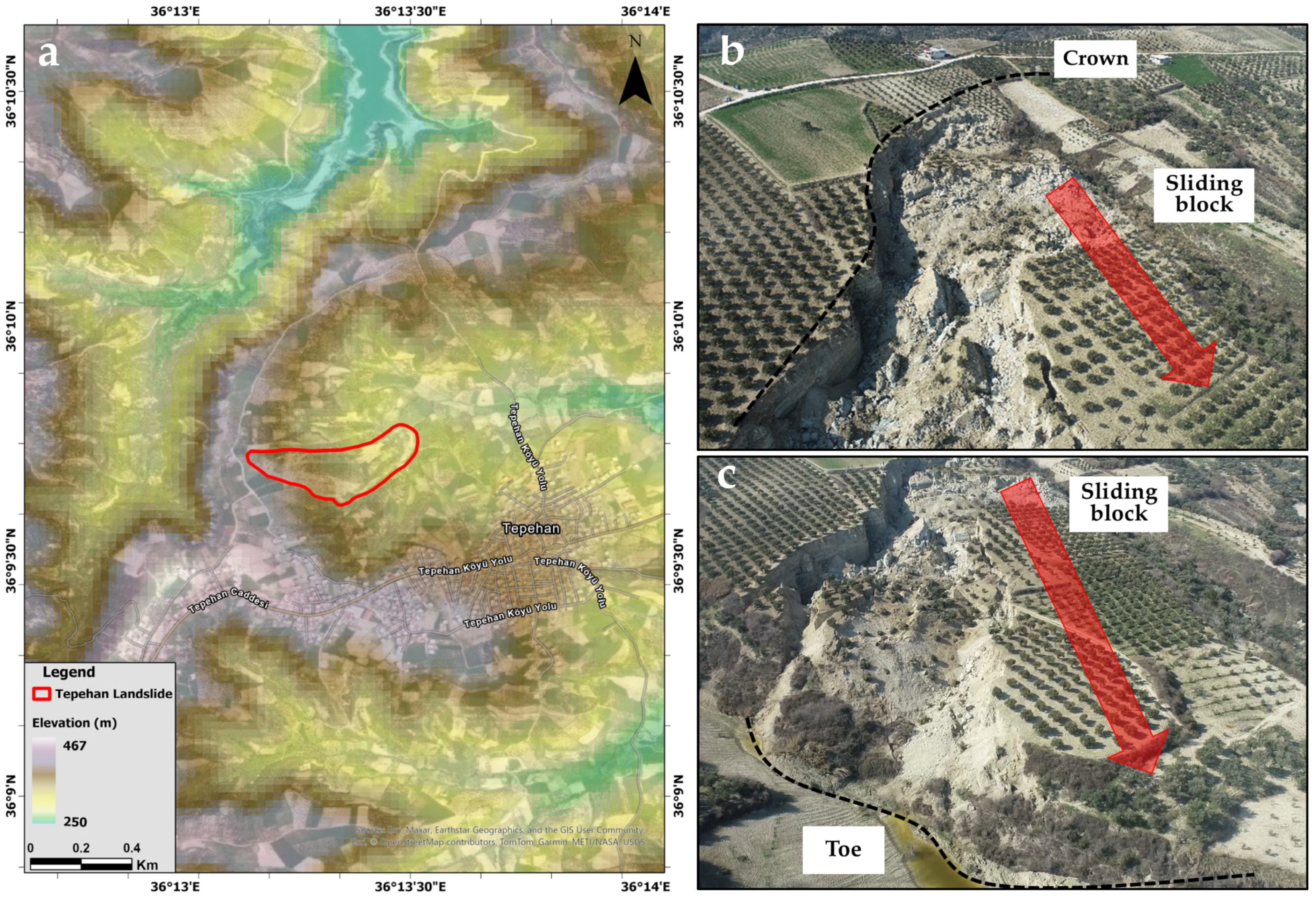
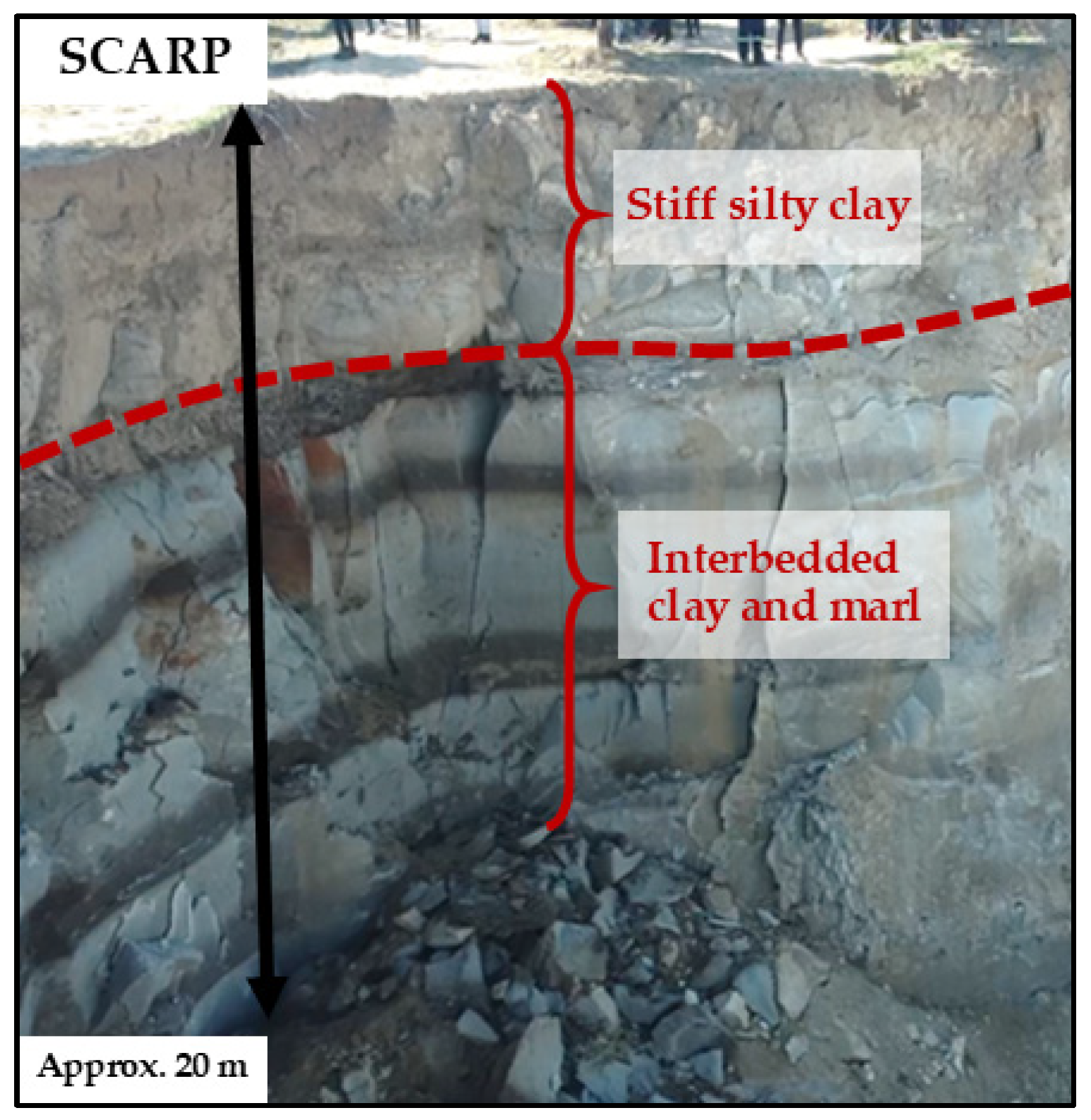
2.1. Site Description
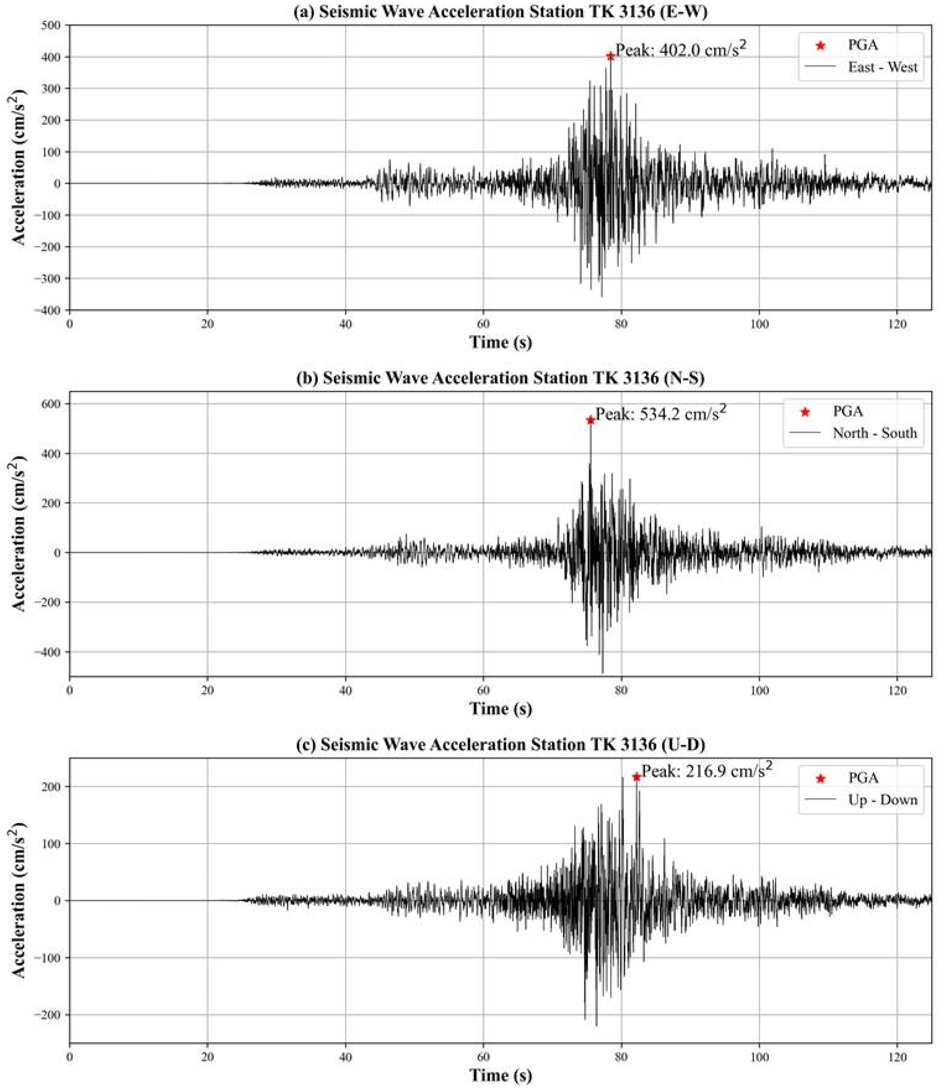
2.2. Earthquake Parameters
3. Methods
3.1. Geomorphometric Analysis
3.2. InSAR DEM
3.3. Slope Stability Analysis Through Back-Analysis
4. Geomorphometric Analysis
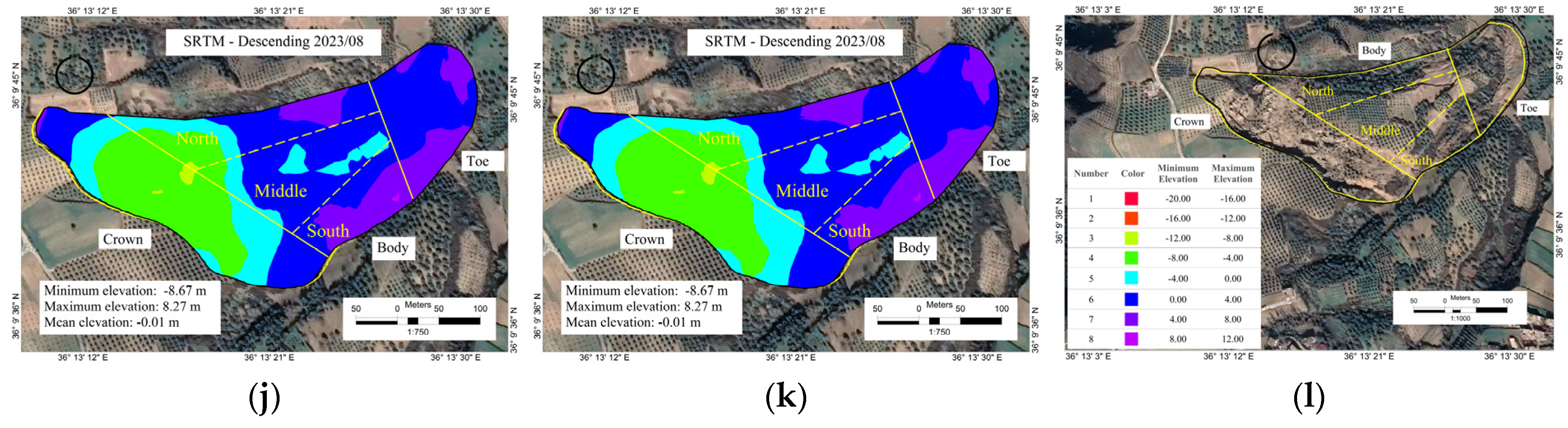
4.1. Topographic Analysis
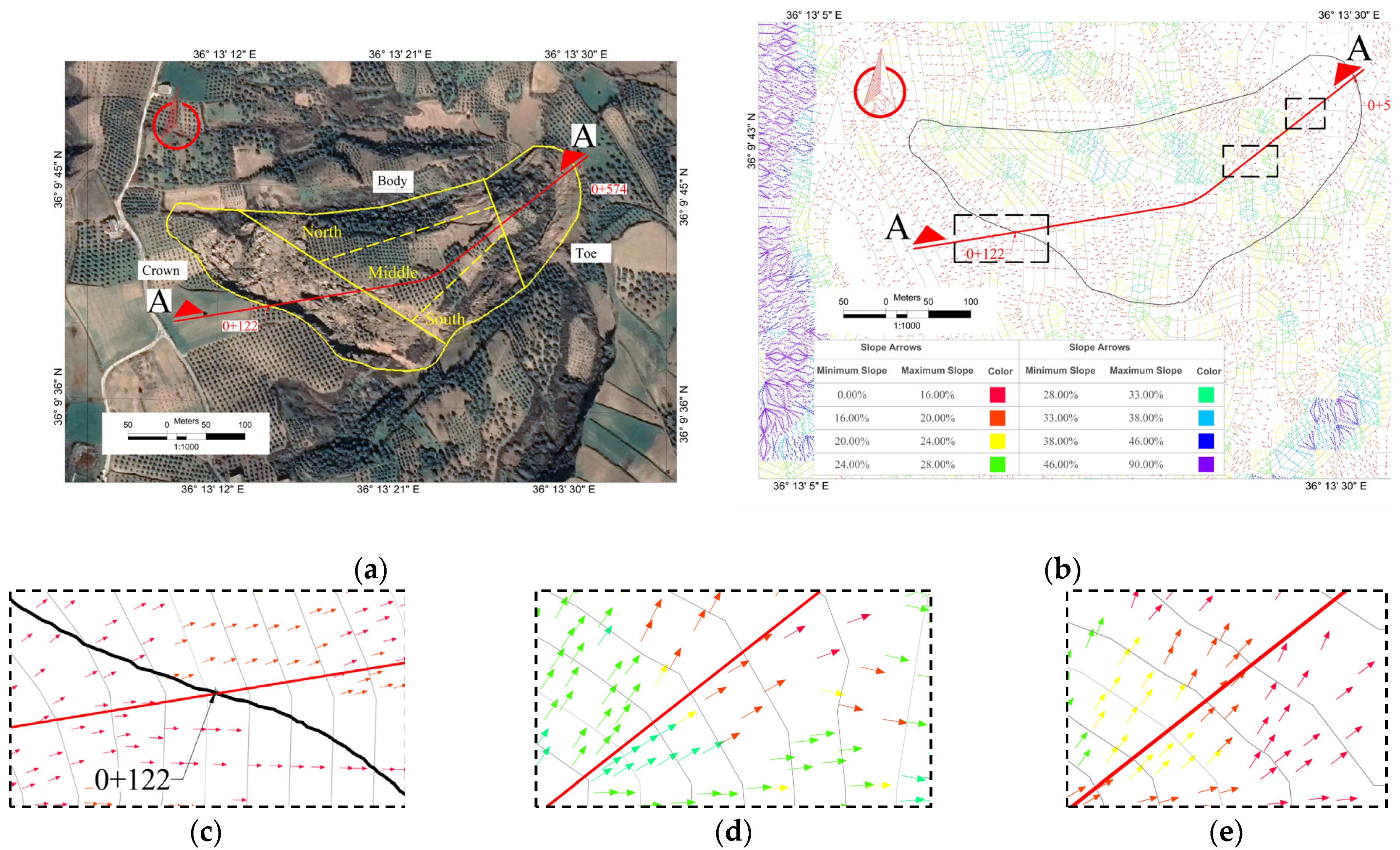
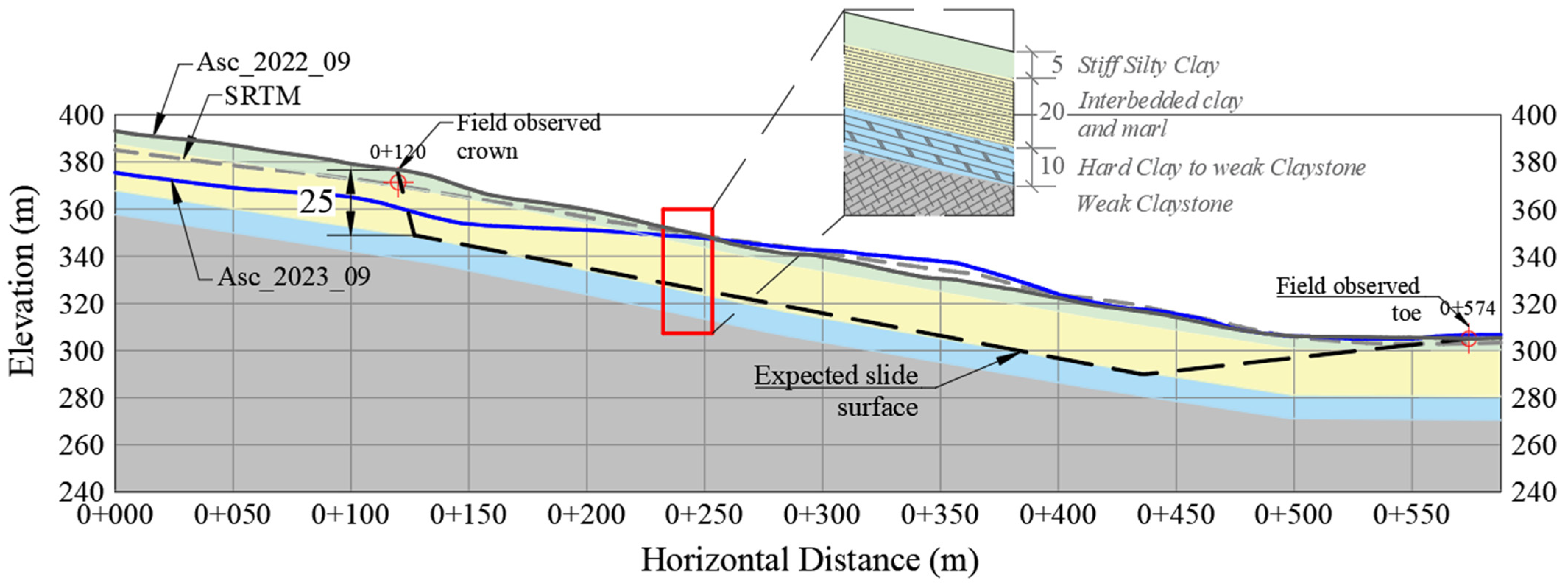
4.2. Defining the Critical Profile for the Static and Pseudo-Static Stability Analysis
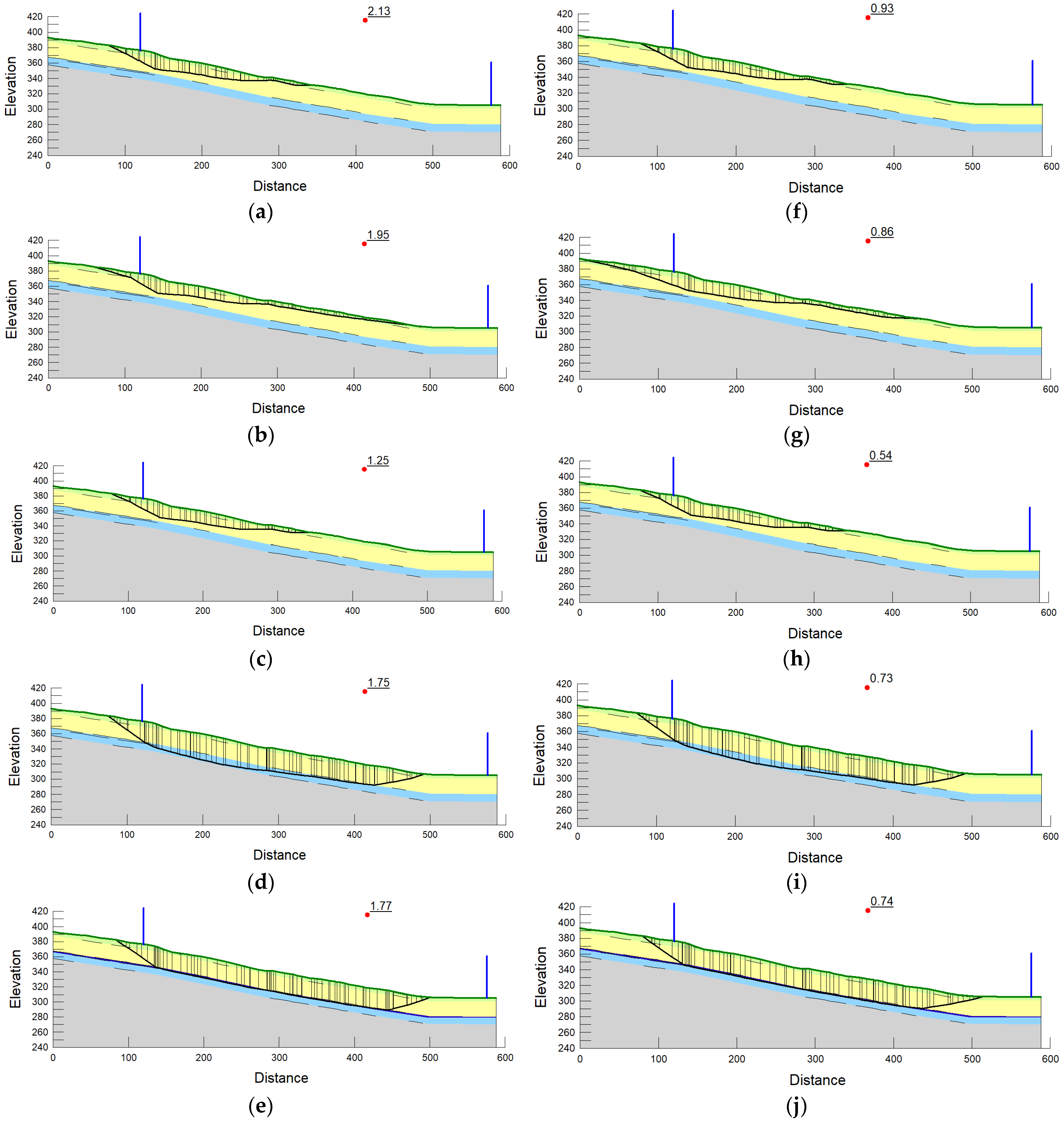
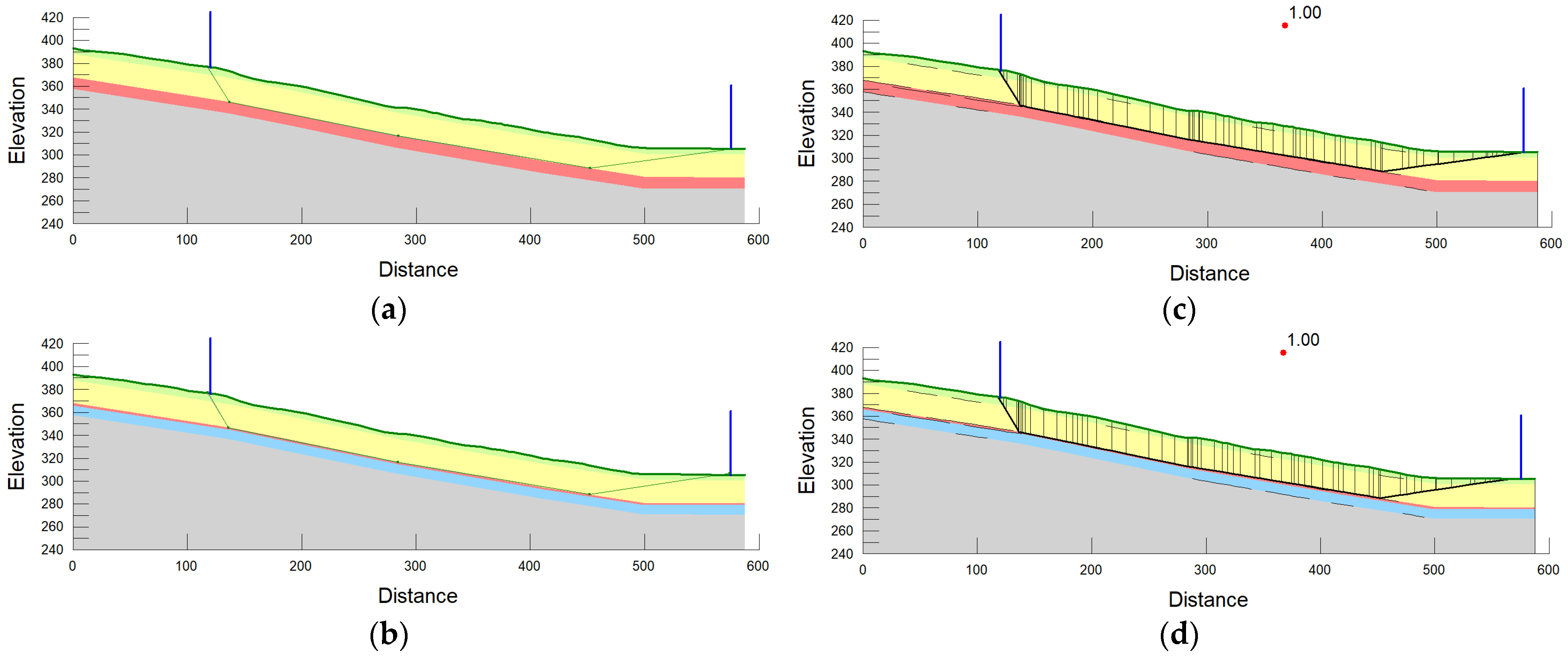
5. Limit Equilibrium Analysis
6. Conclusions
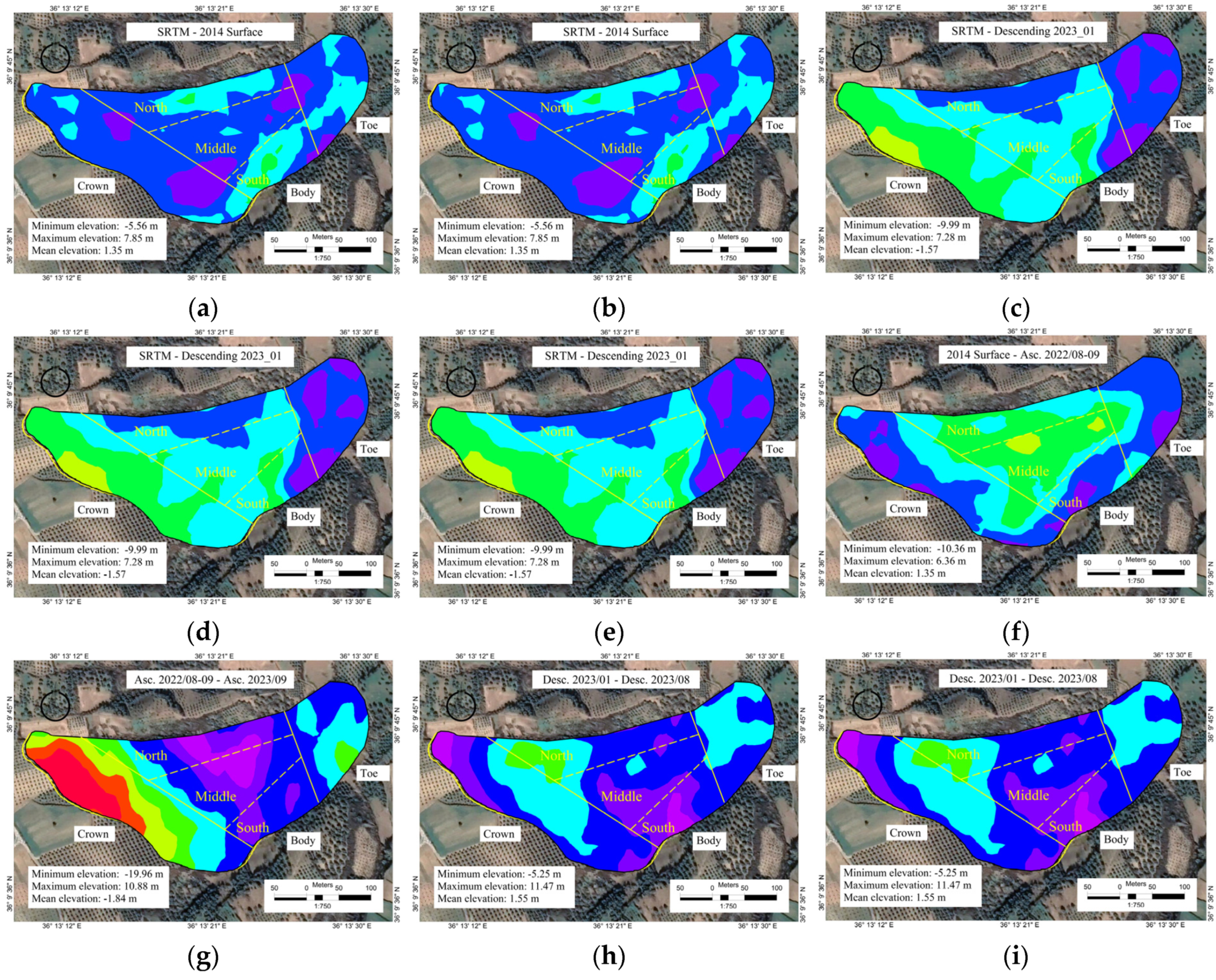
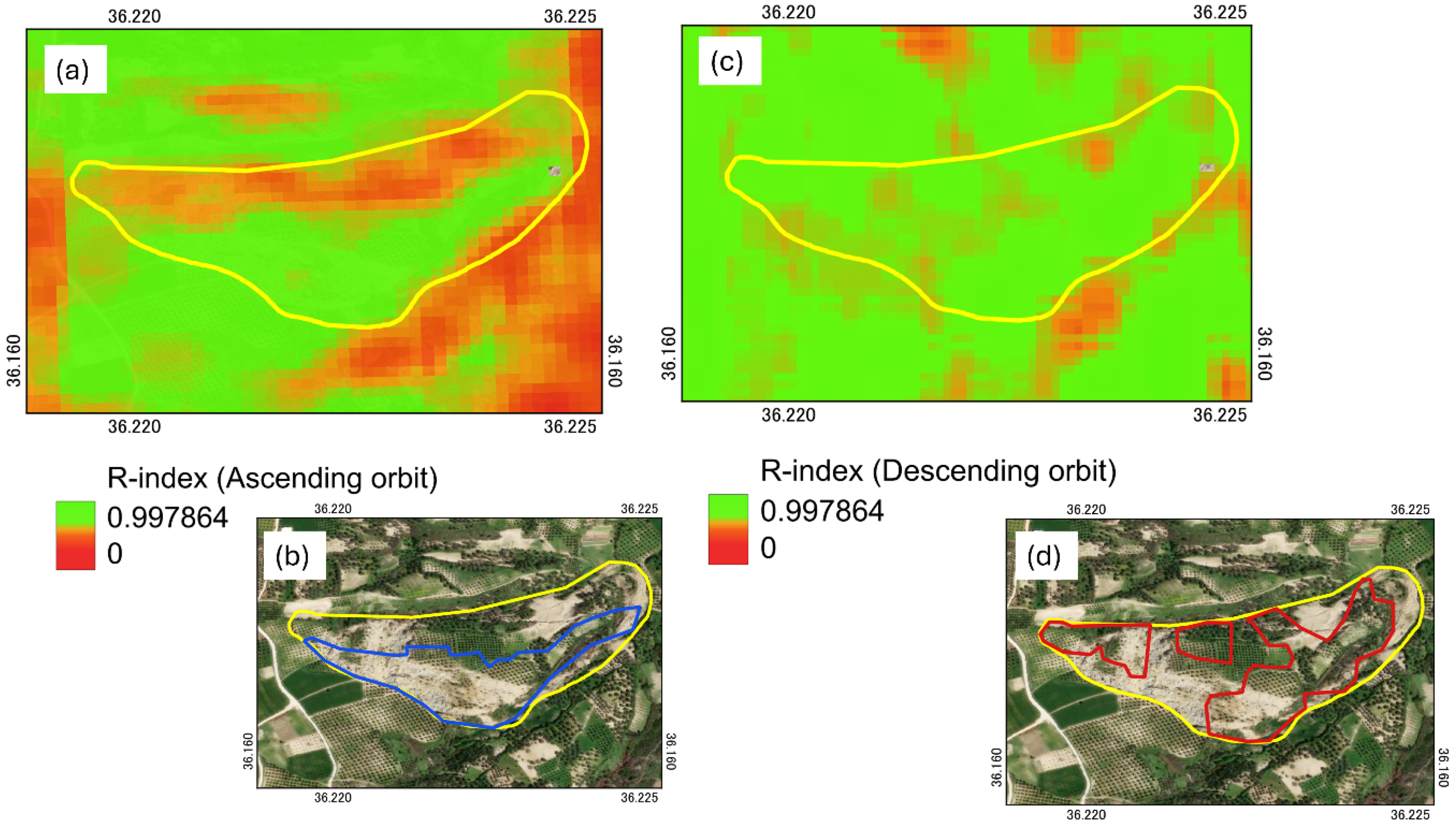
- Topographic variations in the landslide area were analyzed using digital elevation models (DEMs) derived from ascending and descending orbits of Sentinel-1 SAR data. SAR images from the ascending orbit showed a high R-index (line of sight sensitivity), particularly at the landslide crown. Thus, the DEM generated from the ascending orbit SAR data captured the elevation change more accurately, compared to the SAR images of the Sentinel-1 descending orbit track.
- Overall, the soil stratigraphy is well-founded, based on geological history and existing site descriptions, allowing for a reasonable slope profile simulation. Discrepancies between the assumed soil layers and the detailed site investigations can be addressed by sample testing and comparison with assumed parameters.
- The depth of the slip surface reaches from 27 m to 35 m depending on the thickness of the residual bedding layer, from a thin layer in Scenario 5 to a 10 m layer in Scenario 4, respectively. Although the depth variation is significant, it is not a fixed measure. Nevertheless, both scenarios showed very close values of the FoS in static and pseudo-static conditions. Consequently, variations in the slip surface depth within the 20 m to 30 m range, as found in the literature, will not significantly impact the limit equilibrium analyses.
- The analyzed scenarios indicate that the slope behaves as a delayed first-time landslide. The bedding plane in the hard clay acts as a stratigraphic discontinuity, reducing the mobilized shear strength and creating paths for localized shearing strain. This leads to residual conditions and an overall weakening of the slope materials.
- Although the strength parameters were defined using a limit equilibrium pseudo-static approach, the soil stratigraphy and fully softened friction angles, along with the adjusted friction angle for the hard clay layer from 16° to 21°, remain applicable for future investigations of site behavior. Additionally, these parameters can be further refined through more detailed numerical approaches.
Author Contributions
Funding
Data Availability Statement
Acknowledgments
Conflicts of Interest
References
- Karslı, H.; Babacan, A.E.; Akın, Ö. Subsurface characterization by active and passive source geophysical methods after the 06 February 2023earthquakes in Turkey. Nat. Hazards 2024, 120, 5257–5286. [Google Scholar] [CrossRef]
- Yan, K.; Miyajima, M.; Kumsar, H.; Aydan, Ö.; Ulusay, R.; Tao, Z.; Chen, Y.; Wang, F. Preliminary report of field reconnaissance on the 6 February 2023 Kahramanmaras Earthquakes in Türkiye. Geoenviron. Disasters 2024, 11, 1–24. [Google Scholar] [CrossRef]
- Görüm, T.; Tanyas, H.; Karabacak, F.; Yılmaz, A.; Girgin, S.; Allstadt, K.E.; Süzen, M.L.; Burgi, P. Preliminary documentation of coseismic ground failure triggered by the February 6, 2023 Türkiye earthquake sequence. Eng. Geol. 2023, 327, 107315. [Google Scholar] [CrossRef]
- GEER Association. Türkiye Earthquakes: Report on Geoscience and Engineering Impacts. Earthquake Engineering Research Institute, LFE Program GEER Association Report; GEER Association: Kansas City, MO, USA, 2023. [Google Scholar] [CrossRef]
- Dölek, İ.; Uzelli, T.; Ege, İ.; Çelik, Ö. An example of mass movements caused by the Kahramanmaraş earthquakes of february 6: Tepehan landslide. Türk Coğrafya Dergisi 2023, 83, 73–86. [Google Scholar] [CrossRef]
- Milev, N.; Tobita, T.; Kiyota, T.; Shiga, M. Rapid detection of landslides mechanisms and assessment of their geometry and dimensions by means of a drone survey (UAV) after the 2023 Turkey-Syria earthquake. National Transport Infrastructure Conference with International Participation. IOP Conf. Ser. Mater. Sci. Eng. 2023, 1297, 012009. [Google Scholar] [CrossRef]
- Medhat, N.I.; Nieto, K.; Numanoglu, O.A.; Baser, T. Revealing failure mechanisms of the Tepehan landslide using satellite-borne InSAR data. In Proceedings of the 18th World Conference on Earthquake Engineering (WCEE2024), Milan, Italy, 30 June–5 July 2024. [Google Scholar]
- Tarı, U.; Tüysüz, O.; Genç, Ş.C.; İmren, C.; Blackwell, B.A.; Lom, N.; Tekeşin, Ö.; Üsküplü, S.; Erel, L.; Altıok, S.; et al. The geology and morphology of the Antakya Graben between the Amik Triple Junction and the Cyprus Arc. Geodin. Acta 2014, 26, 27–55. [Google Scholar] [CrossRef]
- Kavuzlu, M. Tectono-Stratigraphy of Altınözü (Antakya) and Its Vicinity. Master’s Thesis, Department of Geological Engineering, Institute of Natural and Applied Sciences, Çukurova University, Çukurova, Turkey, 2006. [Google Scholar]
- The Disaster and Emergency Management Authority (AFAD) of Turkey. Compilation of Data Base for The National Strong-Motion Seismograph Network in Turkey: Report on Seismic and Geotechnical Investigations; The Disaster and Emergency Management Authority (AFAD) of Turkey: Ankara, Turkey, 2006; Seismograph Station AI_029_MAT02. [Google Scholar]
- Bray, J.D.; Travasarou, T. Pseudostatic Coefficient for Use in Simplified Seismic Slope Stability Evaluation. J. Geotech. Geoenviron. Eng. 2009, 135, 1336–1340. [Google Scholar] [CrossRef]
- Baker, R.; Shukha, R.; Operstein, V.; Frydman, S. Stability charts for pseudo-static slope stability analysis. Soil Dyn. Earthq. Eng. 2006, 26, 813–823. [Google Scholar] [CrossRef]
- Seed, H.B. Considerations in the earthquake-resistant design of earth and rockfill dams. Geotechnique 1979, 29, 215–263. [Google Scholar] [CrossRef]
- Marcuson, W.F., III; Franklin, A.G. Seismic Design Analysis Remedial Measures to Improve Stability of Existing Earth Dams (Final Report); Geotechnical Laboratory, U.S. Army Engineer Waterways Experiment Station: Vicksburg, MI, USA, 1983. [Google Scholar]
- Hynes-Griffin, M.E.; Franklin, A.G. Rationalizing the Seismic Coefficient Method; Geotechnical Laboratory, Department of the Army, Waterways Experiment Station, Corps of Engineers: Vicksburg, MI, USA, 1984; Prepared for Department of the Army, US Army Corps of Engineers, Washington, DC.1984. [Google Scholar]
- Melo, C.; Sharma, S. Seismic Coefficients for Pseudostatic Slope Analysis (Paper No. 369). In Proceedings of the 13th World Conference on Earthquake Engineering, Vancouver, BC, Canada, 1–6 August 2004. [Google Scholar]
- Pyke, R. Selection of Seismic Coefficients for Use in Pseudo-Static Slope Stability Analyses; California Division of Mines and Geology: Sacramento, CA, USA, 1991.
- Xiong, L.; Li, S.; Tang, G.; Strobl, J. Geomorphometry and terrain analysis: Data, methods, platforms and applications. Earth-Sci. Rev. 2022, 233, 104191. [Google Scholar] [CrossRef]
- ESRI. Surface Creation Analysis, ArcGIS. 2016. Available online: https://desktop.arcgis.com/en/arcmap/10.3/analyze/commonly-used-tools/surface-creation-and-analysis.htm (accessed on 20 January 2024).
- Zhang, Y.; Meng, X.; Jordan, C.; Novellino, A.; Dijkstra, T.; Chen, G. Investigating slow-moving landslides in the Zhouqu region of China using InSAR time series. Landslides 2018, 15, 1299–1315. [Google Scholar] [CrossRef]
- Mohammed, O.I.; Saeidi, V.; Pradhan, B.; Yusuf, Y.A. Advanced differential interferometry synthetic aperture radar techniques for deformation monitoring: A review on sensors and recent research development. Geocarto Int. 2014, 29, 536–553. [Google Scholar] [CrossRef]
- SARscape. SARscape tutorials–Interferometry, Digital elevation model creation. I NV5 Geospatial. 2023. Available online: https://www.sarmap.ch/index.php/software/sarscape/ (accessed on 1 November 2024).
- Hussain, M.; Stark, T.D.; Akhtar, K. Back-Analysis Procedure for Landslides. In Proceedings of the International Conference on Geotechnical Engineering, Lahore, Pakistan, 5–6 November 2010. [Google Scholar]
- Huang, Y.H. Slope Stability Analysis by the Limit Equilibrium Method: Fundamentals and Methods; ASCE Press: Reston, VA, USA, 2014; pp. 1–376. ISBN 978-0784412886. [Google Scholar]
- Gilbert, R.B.; Wright, S.G.; Liedtke, E. Uncertainty in Back Analysis of Slopes: Kettleman Hills Case History. J. Geotech. Geoenviron. Eng. 1998, 124, 1167–1176. [Google Scholar] [CrossRef]
- GEO-SLOPE International Ltd. Stability Modeling with Geostudio (2004–2021); GEO-SLOPE International Ltd.: Calgary, AB, Canada, 2022. [Google Scholar]
- Towhata, I. Geotechnical Earthquake Engineering; Springer: Berlin, Germany, 2008. [Google Scholar] [CrossRef]
- Koo, R.C.H.; Kong, V.; Tsang, H.H.; Pappin, J.W. Seismic slope stability assessment in a moderate seismicity region, Hong Kong. In Proceedings of the 14th World Conference on Earthquake Engineering, Beijing, China, 12–17 October 2008. [Google Scholar]
- Terzaghi, K.; Peck, R.B.; Mesri, G. Soil Mechanics in Engineering Practice, 3rd ed.; John Wiley and Sons, Inc.: New York, NY, USA, 1996. [Google Scholar]
- Mesri, G.; Shahien, M. Residual Shear Strength Mobilized in First-Time Slope Failures. J. Geotech. Geoenviron. Eng. 2003, 129, 12–31. [Google Scholar] [CrossRef]
- Glade, T.; Crozier, M.; Smith, P. Applying Probability Determination to Refine Landslide-triggering Rainfall Thresholds Using an Empirical “Antecedent Daily Rainfall Model”. Pure Appl. Geophys. 2000, 157, 1059–1079. [Google Scholar] [CrossRef]
- Pike, R.J.; Evans, I.S.; Hengl, T. Geomorphometry: A Brief Guide. In Developments in Soil Science; Elsevier: Amsterdam, The Netherlands, 2009; Volume 33, ISSN 0166-2481. [Google Scholar] [CrossRef]
- Notti, D.; Herrera, G.; Bianchini, S.; Meisina, C.; García-Davalillo, J.C.; Zucca, F. A methodology for improving landslide PSI data analysis. Int. J. Remote. Sens. 2014, 35, 2186–2214. [Google Scholar] [CrossRef]
- Guo, R.; Li, S.; Chen, Y.; Li, X.; Yuan, L. Identification and monitoring landslides in Longitudinal Range-Gorge Region with InSAR fusion integrated visibility analysis. Landslides 2021, 18, 551–568. [Google Scholar] [CrossRef]
- Abramson, L.W.; Lee, T.S.; Rathbun, S.D. Slope Stability and Stabilization Methods; John Wiley & Sons: Hoboken, NJ, USA, 2002. [Google Scholar]
- Skempton, A.W.; Petley, D.J. The strength along structural discontinuities in stiff clays. In Proceedings of the Geotechnical Conference, Oslo, Norway, 1967; Volume 2, pp. 29–46. [Google Scholar]


| Layer No | Description | Depth Location (m) | Thickness (m) |
|---|---|---|---|
| 1 | Stiff Silty Clay | 0–5 | 5 |
| 2 | Interbedded Clay and Marl | 5–25 | 20 |
| 3 | Hard Clay to Weak Claystone | 25–35 | 10 |
| 4 | Weak Claystone | >35 | - |
| ID | Images Dates | Temporal Baseline/Images | Perpendicular Baseline (m) | Sensor/Data | Orbit |
|---|---|---|---|---|---|
| 1 | 2022/08/25 and 2022/09/06 | 12 days | 254 | Sentinel-1 | Ascending |
| 2 | 2023/09/13 and 2023/09/25 | 12 days | 254 | Sentinel-1 | Ascending |
| 3 | 2023/02/09 to 2023/12/30 | 26 images | - | Sentinel-1 | Ascending |
| 4 | 2022/01/09 to 2023/01/28 | 31 images | - | Sentinel-1 | Ascending |
| 5 | 2023/01/05 and 2023/01/17 | 12 days | 190 | Sentinel-1 | Descending |
| 6 | 2023/07/28 and 2023/08/09 | 12 days | 272 | Sentinel-1 | Descending |
| 7 | 2023/02/10 to 2023/12/31 | 23 images | - | Sentinel-1 | Descending |
| 8 | 2022/01/10 to 2023/01/29 | 32 images | - | Sentinel-1 | Descending |
| 9 | 2021/03/22 and 2022/03/21 | 364 days | 156 | PALSAR-2 | Ascending |
| 10 | 2023/03/20 and 2024/03/18 | 363 days | 655 | PALSAR-2 | Ascending |
| 11 | 2014 | - | - | Sentinel-1 | 2014_DEM |
| 12 | ~2000 | - | - | SRTM | - |
| DEM | Min (m) | Max (m) | Mean (m) |
|---|---|---|---|
| SRTM | 301 | 378 | 337 |
| Ascending 2022/08 | 303 | 382 | 337 |
| Ascending 2023/09 | 305 | 368 | 335 |
| Descending 2023/01 | 304 | 374 | 336 |
| Descending 2023/08 | 304 | 383 | 337 |
| Descending SBAS | 294 | 382 | 339 |
| ID | Type | Base Surface | Comparison Surface | Resulting Compared File Name |
|---|---|---|---|---|
| A1 | A | SRTM | 2014 Surface | SRTM–2014 Surface |
| A2 | A | SRTM | Ascending 2022/08–09 | SRTM–Ascending 2022/08–09 |
| A3 | A | SRTM | Descending 2023/01 | SRTM–Descending 2023_01 |
| A4 | A | SRTM | Descending SBAS_Pre | SRTM–Descending SBAS_Pre |
| A5 | A | Ascending 2022/08–09 | Descending 2023/01 | Asc. 2022/08–09–Desc. 2023/01 |
| A6 | A | 2014 Surface | Ascending 2022/08–09 | 2014 Surface–Asc. 2022/08–09 |
| B1 | B | Ascending 2022/08–09 | Ascending 2023/09 | Asc. 2022/08–09–Asc. 2023/09 |
| B2 | B | Descending 2023/01 | Descending 2023/08 | Desc. 2023/01–Desc. 2023/08 |
| B3 | B | SRTM | Ascending 2023/09 | SRTM–Ascending 2023/09 |
| B4 | B | SRTM | Descending 2023/08 | SRTM–Descending 2023/08 |
| C1 | C | Descending 2023/08 | Ascending 2023/09 | Desc. 2023-08–Asc. 2023/09 |
| ID | Compared Surfaces | Crown | Body | Toe | ||
|---|---|---|---|---|---|---|
| North Part | Middle Part | South Part | ||||
| A1 | SRTM–2014 Surface | +4 to 8 m | −2 to 6 m | ±2 m | −2 to 6 m | ±2 m |
| A2 | SRTM– Ascending 2022/08–09 | +4 to 7 m | −5 to 8 m | −2 to 6 m | ±2 m | ±2 m |
| A3 | SRTM– Descending 2023_01 | −4 to 9 m | ±2 m | ±2 m | +4 to 7 m | +3 to 6 m |
| A4 | SRTM– Descending SBAS_Pre | 0 to 5 m | ±2 m | ±2 m | +3 to 10 m | ±2 m |
| A5 | Asc. 2022/08–09– Desc. 2023/01 | −5 to 15 m | +2 to 8 m | +2 to 8 m | −2 to 8 m | +2 to 6 m |
| A6 | 2014 Surface– Asc. 2022/08–09 | +2 to 6 m | −2 to 6 m | −4 to 10 m | +2 to 4 m | +2 to 4 m |
| B1 | Asc. 2022/08–09– Asc. 2023/09 | −5 to 20 m | 0 to 10 m | +0 to 10 m | +2 to 6 m | −2 to 5 m |
| B2 | Desc. 2023/01– Desc. 2023/08 | 0 to 5 m | 0 to 5 m | 0 to 5 m | +4 to 10 m | −2 to 3 m |
| B3 | SRTM– Ascending 2023/09 | −2 to 15 m | ±2 m | ±2 m | ±2 m | −2 to 5 m |
| B4 | SRTM– Descending 2023/08 | −2 to 15 m | 0 to 5 m | +4 to 5 m | +2 to 6 m | ±2 m |
| C1 | Desc. 2023_08– Asc. 2023/09 | 0 to 10 m | +2 to 5 m | ±2 m | +2 to 8 m | +2 to 6 m |
| # | Scenario | Layers | Condition | Ø’ (°) | γ (kN/m3) |
|---|---|---|---|---|---|
| 1. | First-time landslide | Stiff Silty Clay | Fully Softened | 22 | 18 |
| Interbedded Clay and Marl | Fully Softened | 23 | 19 | ||
| Hard Clay to Weak Claystone | Fully Softened | 25 | 20 | ||
| 2. | Reactivation of the first layer and the first-time landslide downward | Stiff Silty Clay | Residual | 13 | 18 |
| Interbedded Clay and Marl | Fully Softened | 23 | 19 | ||
| Hard Clay to Weak Claystone | Fully Softened | 25 | 20 | ||
| 3. | Reactivation landslide | Stiff Silty Clay | Residual | 13 | 18 |
| Interbedded Clay and Marl | Residual | 14 | 19 | ||
| Hard Clay to Weak Claystone | Fully Softened | 25 | 20 | ||
| 4. | Delayed first-time landslide—subsurface residual layer | Stiff Silty Clay | Fully Softened | 22 | 18 |
| Interbedded Clay and Marl | Fully Softened | 23 | 19 | ||
| Hard Clay to Weak Claystone | Residual | 16 | 20 | ||
| 5. | Delayed first-time landslide—subsurface residual thin weak layer | Stiff Silty Clay | Fully Softened | 22 | 18 |
| Interbedded Clay and Marl | Fully Softened | 23 | 19 | ||
| Weak Layer | Residual | 16 | 20 | ||
| Hard Clay to Weak Claystone | Fully Softened | 25 | 20 |
| Scenario | FoS for Static Analysis | FoS for Pseudo-Static Analysis | Maximum Depth of Slip Surface (m) |
|---|---|---|---|
| 1 | 2.13 | 0.93 | 20 |
| 2 | 1.95 | 0.86 | 20 |
| 3 | 1.25 | 0.54 | 20 |
| 4 | 1.75 | 0.73 | 35 |
| 5 | 1.77 | 0.74 | 27 |
| Layers | Color | Condition | Back-Calculated Ø’ (°) | γ (kN/m3) |
|---|---|---|---|---|
| Stiff Silty Clay |  | Fully Softened | 22 | 18 |
| Interbedded Clay and Marl |  | Fully Softened | 23 | 19 |
| Hard Clay to Weak Claystone |  | Fully Softened | 27 | 20 |
| Hard Clay to Weak Claystone |  | Residual | 21 | 20 |
| Weak Claystone |  | - | - | 20 |
Disclaimer/Publisher’s Note: The statements, opinions and data contained in all publications are solely those of the individual author(s) and contributor(s) and not of MDPI and/or the editor(s). MDPI and/or the editor(s) disclaim responsibility for any injury to people or property resulting from any ideas, methods, instructions or products referred to in the content. |
© 2025 by the authors. Licensee MDPI, Basel, Switzerland. This article is an open access article distributed under the terms and conditions of the Creative Commons Attribution (CC BY) license (https://creativecommons.org/licenses/by/4.0/).
Share and Cite
Nieto, K.; Medhat, N.I.; Yusupujiang, A.; Sagan, V.; Baser, T. Stability Assessment of the Tepehan Landslide: Before and After the 2023 Kahramanmaras Earthquakes. Geosciences 2025, 15, 181. https://doi.org/10.3390/geosciences15050181
Nieto K, Medhat NI, Yusupujiang A, Sagan V, Baser T. Stability Assessment of the Tepehan Landslide: Before and After the 2023 Kahramanmaras Earthquakes. Geosciences. 2025; 15(5):181. https://doi.org/10.3390/geosciences15050181
Chicago/Turabian StyleNieto, Katherine, Noha I. Medhat, Aimaiti Yusupujiang, Vasit Sagan, and Tugce Baser. 2025. "Stability Assessment of the Tepehan Landslide: Before and After the 2023 Kahramanmaras Earthquakes" Geosciences 15, no. 5: 181. https://doi.org/10.3390/geosciences15050181
APA StyleNieto, K., Medhat, N. I., Yusupujiang, A., Sagan, V., & Baser, T. (2025). Stability Assessment of the Tepehan Landslide: Before and After the 2023 Kahramanmaras Earthquakes. Geosciences, 15(5), 181. https://doi.org/10.3390/geosciences15050181