Abstract
This study investigates co-seismic landslides triggered by the 1 January 2024 Mw 7.6 Noto Peninsula earthquake in Japan using LiDAR differentiation and a modified Savage–Hutter model. By analyzing pre- and post-earthquake high-resolution topographic data from 13 landslides in a geologically homogeneous area of the peninsula, we characterized distinct landslide morphologies and dynamic behaviours. Our approach combined static morphological analysis from LiDAR data with simulations of granular flow mechanics to evaluate landslide mobility. Results revealed two distinct landslide types: those with clear erosion-deposition zonation and complex landslides with discontinuous topographic changes. Landslide dimensions followed power-law relationships (H = 7.51L0.50, R2 = 0.765), while simulations demonstrated that internal deformation capability (represented by the μ parameter) significantly influenced runout distances for landslides terminating on low-angle surfaces but had minimal impact on slope-confined movements. These findings highlight the importance of integrating both static topographic parameters and dynamic flow mechanics when assessing co-seismic landslide hazards, particularly for predicting potential runout distances on gentle slopes where human settlements are often located. Our methodology provides a framework for improved landslide susceptibility assessment and disaster risk reduction in seismically active regions.
1. Introduction
1.1. Background
Co-seismic landslides have long been recognized as an issue during earthquakes [1], with the seismic intensity controlling the spatial distribution of landslides [2,3]. Co-seismic landslides are a common occurrence in the islands and archipelagos surrounding the Pacific (e.g., New Zealand [4], Indonesia [5], the Philippines [6], Taiwan [7,8], Japan [9]). Extending to the West coast of South America, it is a geographic ribbon wrapping the Pacific Ocean known as the earthquake hotspot for events > Mw 6.0 [10]. This unenviable record has earned this strip of land and sea the name of “Ring of Fire”.
The important seismic activity is accompanied by rapid uplift (New Zealand Alps, Japanese Alps) and the preferable formation of stratovolcanoes (Merapi, Semeru, Fuji), which are steep-sloped mountains. In combination with the proximity of active faults [11,12], steep slopes make for terrains prone to co-seismic landslides. Adding to this tectono-geomorphologic setting, the combination of monsoon, typhoons, seasonal rains [13], heavy snow-falls, as well as an increase in climate-change-concentrated heavy rainfalls all contribute to the landslide susceptibility by (1) creating deeply weathered soils and (2) and contributing to the instability by adding water to the slopes before seismic events or triggering landslides after initial seismic destabilization. Co-seismic landslides present complex triggering mechanisms involving both dynamic loading and ground motion cycles [14,15], as the seismic acceleration increases shear stress along the potential sliding surface while weakening the soil structure [16]. Furthermore, it modifies the traditional depth-dependence of soil shear-strength on slopes, introducing other spatial dependences like the distance to active faults [17]. Finally, there have also been reports that co-seismic landslides can travel longer distances [18] than rainfall landslides.
In turn, co-seismic landslides have profound impacts on the environments—referred to as Earthquake Environmental Effects (EEEs) [19]—which have been shown to recur at the same locations over historical time (e.g., in Indonesia [20]). These effects are now being assessed in greater complexity thanks to a new scale: the Environmental Seismic Intensity (ESI) scale, notably introduced by Serva et al. [19], which includes a broader range of information, including human experiences of earthquakes.
The investigation of landslides is therefore essential for scientists and engineers who try to unravel their mechanisms, local population living with and on those terrains, as well as the authorities and stakeholders involved in the management related and integrating landslides. The first account of landslides left in the Western tradition dates back to Ancient Greece, around 372–371 BCE [21], with the first “scientific” account in Calabria (Italy) in 1783 [22]. Past landslides have then been unearthed by later researchers, notably using statistical approaches:, e.g., the 1935 New Guinea Mw 7.9 co-seismic landslides [23], historical Northern California earthquakes [24], and New Zealand earthquakes [25]. In the face of the difficulty of defining deterministic physical models, scientists have heavily researched data-driven models and projection [26]. High-quality landslide inventories that comprise seismic factors (PGA, intensity), geological features (faults, lithology), geomorphometric features (elevation, slope, aspect), hydrological characteristics (river erosion, rainfall) and environmental characteristics (land use, etc.) have been shown to be essential for hazard assessment [27].
As the scientists’ toolbox has increased in size and become more diversified (e.g., the ESI scale for EEEs [19]), multiple-scale acquisition platforms now complement the aerial photographs used in early research [23]. Satellite imagery like Sentinel-2 can used to achieve rapid, high-quality (>85% accuracy) mapping [28], and Synthetic Aperture Radar (SAR) platforms also offer mapping possibilities even with clouded skies [27]. Closer to the ground, LiDAR (Light Detection And Ranging) on airplanes have provided unrivalled sample density, precision and accuracy at the local to regional scale [29,30]. It has improved landslide mapping [31], even under forest-cover [32], and high-resolution DEMs and their derivatives [33] have been increasingly analyzed to build landslides’ inventories. This has provided the opportunity to rapidly develop comprehensive databases of landslides’ morphology [34]. Furthermore, the democratization of UAVs (Unmanned Aerial Vehicles) over the last 20 years has enabled the detailed recording of single to few local events [35,36], even though issues such as vegetation occlusion [37,38] and intrinsic errors when surveying complex targets are still not fully understood [39].
Thanks to advances in data acquisition, landslide inventories have expanded significantly following recent seismic events, enabling comparisons of local contributing factors with global databases of case studies (e.g., in New Zealand [40]).
Most geospatial approaches to landslide susceptibility have attempted to calculate various probabilistic indicators from static information or simplified block-sliding models, such as the Newmark method [41,42]. However, these approaches often conceal the complex interactions occurring during slope failure. This comes notably from the difficulty to create suitable models [27], ones that are neither too computationally intensive nor lacking calibration against laboratory experiments. The Newmark displacement model dates back to 1965. It calculates the cumulative permanent displacement of a rigid sliding block. It represents the minimum acceleration required to overcome the static friction forces stopping the slopes from sliding. This method has since been extended for more complex representations of the sliding blocks and adapted to various types of landslides [43,44,45]. It became the link between the earlier static approaches like the limit equilibrium methods, and more advanced Finite Element and Finite Difference Methods [46], and Discrete Element Methods like Smooth Particle Models [47]. These methods are, however, well suited for a single landslide but become very computationally intensive if one wanted to apply them to several landslides. Furthermore, the setup is more time-consuming and complicated than for the two first methods. Finally, probabilistic and GIS-based models (e.g., [48,49]) may complete this toolbox, but they suffer from the lack of in-depth knowledge of the micro-conditions on each slope, so that significant errors always remain in the results. Furthermore, the complexity of relating landslides to earthquake characteristics has proven to not be a straightforward matter, as similar magnitude earthquakes within a single region have been shown to have very different effects (e.g., the Ms 6.6 Jinggu earthquake triggered 441 landslides, while the Ms 6.5 Ludian earthquake caused 10,559 landslides [50]).
Because scientists have proposed that local variability may thus be more of a control on landslides movement, the present work aims to contribute to this research gap by researching landslides’ parameters relevant to the in-motion mechanic using a dynamic model modified from the Savage–Hutter model calibrated against pre- and post-earthquake LiDAR topography, within a small area to identify the role of local parameters in a seemingly homogeneous topography, geology, and distance from the epicentre.
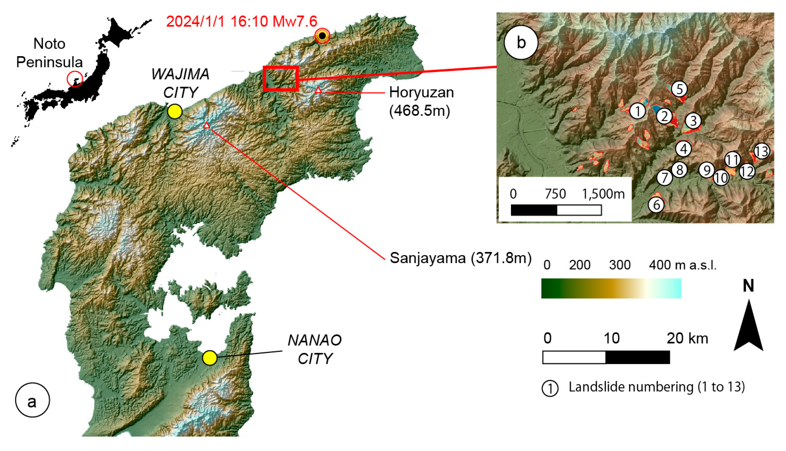
To reach this objective, the present study investigated a set of shallow landslides (translational debris and earth slides) in a topographically and geologically homogeneous area of the Noto Peninsula, Japan (Figure 1), following the 1 January 2024 Noto Peninsula Earthquake.

Figure 1.
Research location on the Noto Peninsula, mapped from a 10 m resolution DEM. Panel (a) depicts the full topography of the peninsula, highlighting the two major cities and the epicentre of the 1 January 2024 earthquake. The landslides analyzed in the present study, extracted from LiDAR data, are mapped in the zoomed-in view provided in panel (b). The large yellow dots mark the location of the cities, the small ones the location of local mountain peaks, and the yellow dot with a black center marks the location of the epicenter.
1.2. Research Location
The earthquake interrupted the celebration of New Year’s Day with a Mw 7.6 event at 16:10 local time that lasted for about 40 s, with the main shock being triggered by a NE–SW trending thrust-fault [51]. The event has been shown to be the tail of an earthquake swarm that started in November 2020 [52], which ended by an unexpectedly strong event, or ‘dragon king’ event [53], and also followed a Mw 6.3 earthquake in 2023, the Oku-Noto Earthquake [54]. The epicentre of this earthquake was located to the North, near the tip of the peninsula (Figure 1) and 11 km from the research location. The peninsula is characterized by a series of low-rising mountains ranging between 300 m and 500 m in elevation, along with plateaux at 80 m a.s.l., which, like the mountain ranges, are deeply incised, with occasional wider valleys associated with fault lines [55].
Geologically, the Noto Peninsula is composed of Neogene volcaniclastic and sedimentary rocks, which overlay Paleozoic to Mesozoic basement rocks [56]. The foot of the peninsula (the southern part) is mainly composed of Neogene formations (Early Miocene to late Pliocene). Over these formations, Quaternary sediment formations of marine terraces and alluvial deposits in the large graben area [57] visible to the South, ending at Nanao City (Figure 1). The study area (Figure 1b), where the landslides are located, is made of Neogene Miocene marine siliceous mudstone. Landslides to the south, lovated above 300 m a.s.l., originate from a Miocene pyroclastic rock formation. The geological characteristics of the location influenced the choice of the survey area, allowing for theuse of relatively homogeneous formations and limiting the complexity of the simulations (for geological maps, see Ozaki [55]).
2. Materials and Methods
Arguably, one of the main difficulties when working with the soil parameters relevant to a co-seismic landslide is that pre-earthquake and post-earthquake soil conditions are not the same, neither just after the earthquake nor during the material flow. Indeed, as the P-waves first send compression and decompression waves that modify the soil structure (i.e., internal friction angle and moisture ratio, etc.), the conditions measured pre-earthquake are not the ones landslide researchers are interested in. Secondly, as liquefaction occurs during the flow, and because direct observations and measures are difficult to obtain, there is a need to integrate the dynamic components occurring on a slope to compare landslides.
In the present contribution, the methodology is twofold. First, the authors analyzed the static slopes from LiDAR differentiation, and then using the geometry obtained from the LiDAR data, the authors ran a granular flow model to try to identify the variability of parameters necessary to reproduce the observed landslides. Using similar sets of mechanical characteristics for each landslide, allow us to define a hierarchy of mobility by accounting for the influence the flow mechanics may have on the flow. For this purpose, a simplified Savage–Hutter model with a synthetic parameter mu and a ground-friction parameter was programmed. The Savage–Hutter model is an adaptation of a shallow-water model, accounting for the forces interacting in a granular media flowing on slopes. The present contribution is thus articulated around a two-step approach with first the LiDAR data analysis and second the simulations (Figure 2), both contributing to the characterization of the co-seismic landslides.
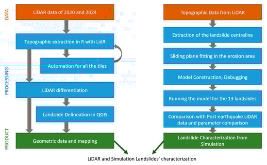
Figure 2.
Methodological flow chart of the present study (LiDAR: Light Detection and Ranging; R stands for the R language; QGIS: Quantum Geographic Information System).
2.1. Pre- and Post-Earthquake LiDAR Analysis and Landslide Morphology Retrieval
The Noto Peninsula is partially covered by several partial LiDAR datasets, before and after the earthquake. Prior to the earthquake, the survey location (Figure 1) was covered by a LiDAR dataset generated four years before the earthquake (Y2020) for forestry purposes by AeroAsahi, Ltd. (Tokyo, Japan) for the prefecture of Ishikawa. The LiDAR data collected after the 2024 earthquake is a courtesy of Kokusai-Kogyo Ltd. (Tokyo, Japan), which generated a 10 pts/m2 density data collected between 13 and 17 January 2024.
For the present contribution, the authors extracted the ground values by classifying the point-cloud using the clothing algorithm of [58]. This algorithm provides an effective way to retrieve the bare ground by separating the vegetation and anything above the ground level. The task was automated with the R programming language in R-Studio-524, using the LidR library. In the same programme sequence, the classified points were tinned and a 1 m horizontal resolution DEM (Digital Elevation Model) was generated. Then, the DEM tiles were processed further in the QGIS3.4 software to (1) extract the morphological characteristics of the landslides to define the objects to be simulated (Distance travelled (L), Height drop (h), their ratio (h/L), the Factor of Safety (Fs), and positioning parameters) and to (2) extract the landslides centrelines used to generate the simulations.
Furthermore, a simplified factor of safety was calculated at landslides’ locations before and after they occurred. Because the earthquake occurred in the midst of winter, the assumption was made that the groundwater did not play a major role, and the landslides were selected within a single geological formation and limited distance so that the calculation was made from the critical slope thresholds.
2.2. Simulation Model
The model used in the present contribution is an adapted Savage–Hutter model, which has been a popular solution for simulating granular flows, including landslides [59], laboratory and natural debris-avalanches [60], and debris-flows [61], as well as mass-movements triggering tsunamis [62]. It differs from the shallow-water equation as it includes terms that account for the internal friction between the grains using a Coulomb Model. It includes a mass conservation equation (Equation (1)) and a momentum conservation equation (Equation (2)).
where is the flow depth; is the depth-averaged velocity; g is the gravitational acceleration; z is the ground elevation; is the total friction forces; and is the seismic force, which is set as a starting acceleration in the model and is not lasting during the flow as the liquefaction state of the flow is less or not conductive to the shear-waves.
The friction force combines (Equation (3)) a velocity dependent term (Equation (4)) and the Coulomb friction term (Equation (5)) as follows:
The seismic forcing is empirically added as a function of g as a start of acceleration.
The numerical implementation of this set of equation is based on a Lax–Friedrichs scheme for flux computation, with a Courant–Friedrich Number of 0.25 and a space step ~0.25 m (small variation occurs as the real space is divided into a n number of cells for each landslide). The transition between wet and dry land during computation was handled using a minimum flow height of 1 mm.
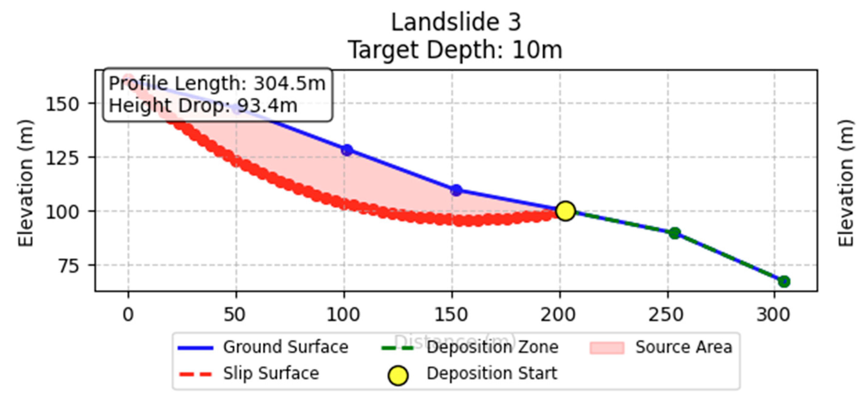
The landslides were simulated using a sliding plane defined below the erosion zone, and in the deposition zone at the bottom of the landslide the material was set to flow on a simplified pre-earthquake topography (example of the setup for landslide 3: Figure 3).
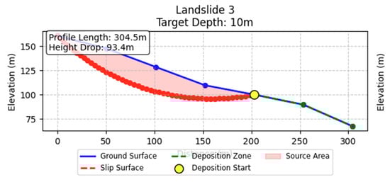
Figure 3.
Landslide setup with a maximum sliding plane at a 10 m depth.
The physical model was parameterized using the Nelder–Mead optimization algorithm, with a starting parameter at 34 degrees, which was the minimum angle of friction for the landslides not to move without seismic acceleration. From this value, angles were tested to reproduce the closest distance travelled by the landslides using the physical model. The termination criteria for the algorithm were set for 100 iterations with a solution expressed as the tangent of the angle varying by less than 0.001. As the landslide is set in movement, and the shear strength reduced, it was assumed that the friction angle is reduced, therefore the algorithm investigated angles below 34 degrees. This iteration was repeated for a set of mu parameters, tested with sets of values of 0.1, 0.2, 0.3, 0.4, and 0.5, chosen based on trial and error, also using the Nelder–Mead algorithm. These values mark the ability of the flow to deform during flow, and thus comparing the shape of the landslide deposit generated at the same time-step, we can compare whether a landslide had to have the ability to “deform more than another” in order to reach its final position.
3. Results
The 13 landslides of the survey area range in altitude between 249 m a.s.l. and 101 m a.s.l. at the landslides’ crown. Downstream, the landslides’ toes are ranging from 102 m a.s.l. to 22 m a.s.l. This variability reflects the position of the landslides in the watershed, as landslides 1, 2, 3, 5, and 13 are on the upper slopes and the others extend down to the valley.
3.1. Erosion and Deposition Analysis from LiDAR Differentiation
The vertical topographic change showing post-event resultant erosion and deposition presents topographic change adding to >40 m per landslides, with deposition zones and erosion zones above +/− 20 m (landslides 1, 2, 3, 4, 5, 6, 13 on Figure 4). Landslides 2, 6, 7, and 12 show a clear differentiation between erosion and deposition, whereas landslides 1, 4, 5, 11, and 13 display discontinuities with accumulations spatially intercalated within a broadly defined erosion area. Landslides 8, 9, and 10 are not proper full-scale landslides, as a general deformation show a topographic increase everywhere, without a clear erosion area, showing the precursor of a landslide. These three landslides are all located on slopes connected to the valley floor and are the landslides with the steepest slopes (31° to 37°), while landslides 4, 6, 7, 11, and 12 have moderate slopes between 20° and 28°, and finally landslides 1, 2, 3, 5, and 13 have slopes between 15° and 17°.
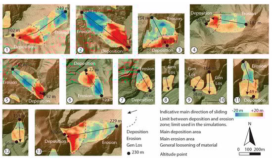
Figure 4.
LiDAR DEM differentiation, before and after the earthquake showing a wide range of displacement types based on the original topography. Each landslide has been numbered between 1 and 13.
As a slope proxy, the authors also expressed the slopes as a synthetic Factor of Safety without cohesion based on the slope and an infinite slope model for a purely granular flow. The results show the hierarchy of slopes with FoS < 1.0 at φ = 20° for landslides 3, 4, 6, 7, 8, 9, 10, 11, and 12 and the FoS, while the upper slope landslides 1, 2, and 13 were >1.03. This distribution logically persists for φ = 25° and 30°. In the group, the landslides 8, 9, and 10 have the lowest FoS, with little variation but yet a slight increase in value (Table 1).

Table 1.
Factor of safety pre- and post-earthquake based on the LiDAR topography and tested internal angle of friction as an estimate of slopes’ effects on stability.
For the centreline of the landslides and comparing the length against the profile volume (2D surface), the relationship is V = 3.39L1.61 (R2 = 0.931), suggesting scaling with the lengths. Longer landslides are also deeper ones, whereas small movements should be more shallow (Figure 5). The relation between the length and the height-drop H provides comparable results for the power-law relationship H = 7.51L0.50 (R2 = 0.765), and the linear relation (graphed with a red line on Figure 5b) with H = 0.2L + 67.34 (R2 = 0.744). Consequently, the height-drop is related to the 2D Volume by V = 0.09H2.62 (R2 = 0.810).
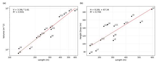
Figure 5.
Morphological parameters relationships: (a) relation between the volume underneath the central line (surface area) and the length (m) of the landslide; (b) relation between the length of the landslide and the vertical drop. The L accompanied with a number are the landslide numbers; H is the vertical drop and V is the volume.
Compared to the pre-earthquake topography, the post-co-seismic landslide topography shows more irregularity with increased roughness (Table 2).
Table 2.
Topographic roughness comparison before and after the earthquake in areas where landslides occurred.
Comparing the values of roughness (Table 2) with the surface change maps (Figure 4), these values reflect the transfer and limited deformation of certain surface features of the landslides. The highest roughness values were associated with the steepest slopes and landslides with thelowest FoS, specifically landslides 8, 9, and 10.
These topographic characterizations, however, are not inclusive of the mechanisms during movement, and to gain insights on the internal processes such as which landslide liquefied more than another did in order to move, we compared different simulation results.
3.2. Simplified Savage–Hutter Landslides’ Simulations
Out of the 13 landslides, the landslide simulation of landslides 2 to 13 worked well, while landslide 1 not sliding out of its position, and mass transfer despite surface deformation (see the Section 4 on this topic).
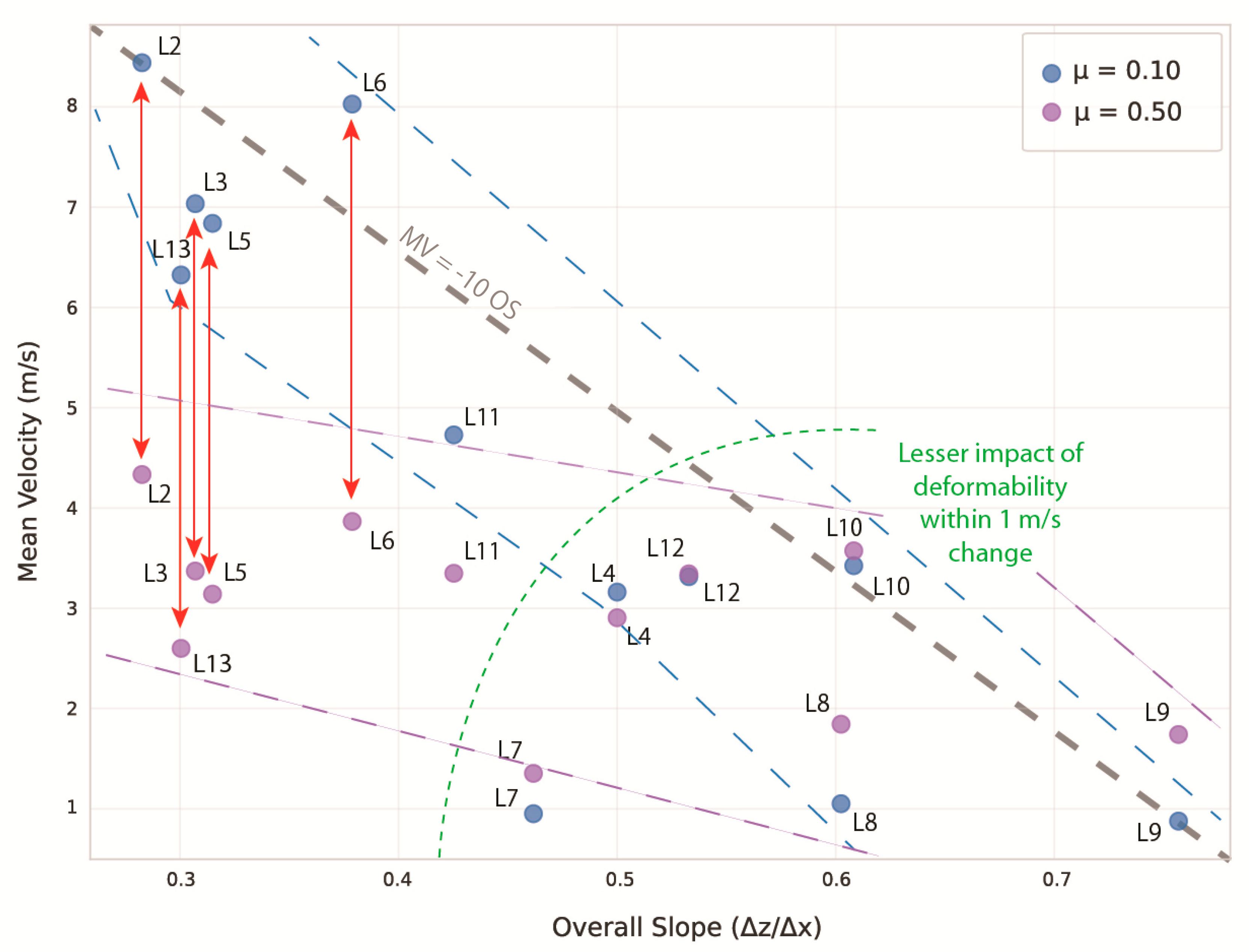
Comparing the minimum and maximum computed μ values (between 0.1 and 0.5) we can divide the landslides into two types. There are those that are driven by the slope with similar results, regardless of the internal deformation: landslides 4, 7, 8, 9, 10, and 12, and those that can show greater variability and thus velocity during flow: landslides 2, 3, 5, 6, 13, and to some extent 11 (Figure 6). These landslides coincide with those occurring on lower-angle topographic slopes (<4.5). It thus demonstrates that the mechanical properties of landslides occurring on steep slopes are different from those on shallow-angle slopes. The group of landslides highly influenced by the mu parameters also all belong to one type of landslides (Figure 4) with a clearly identified erosion zone upstream and a clear accumulation downstream. The other landslides show a more complex surface, with accumulations within the broader erosion area.
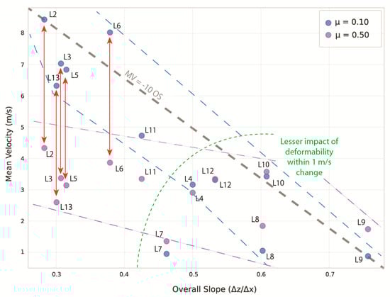
Figure 6.
Impact of internal deformability on landslide motion against the slope angle. The grey doted line is a linear relation between the two variables, whereas the blue and violet dotted lines are indicative limits of the data range. The green dote line limit shows the location where the internal deformability plays a more important role in the landslide movement against the slope importance. The vertical double-headed arrows show visually the variability of potential velocities and thus greater internal deformation depending on the μ coefficient variation.
4. Discussion
4.1. Main Findings
The present study, based on LiDAR differentiation, found that landslides could either display a textbook-like erosion–deposition duality or form more complex landforms. Despite these differences, the relationship between the travel length and total elevation drop revealed a consistent pattern which could be expressed as a power-law relationship: H = 7.51L0.50 (R2 = 0.765) or, alternatively, a linear relationship: H = 0.2L + 67.34 (R2 = 0.744). However, for landslides 2, 3, 5, 6, 13 and to some extent 11, the toe of the landslide reaches a flat valley floor, which decreases the overall slope value of the landslide and highlights the influence of the μ factor, which controls lateral spreading over the flat area. In other words, deformable landslides can spread acrossflat surfaces, but this parameter does not play such an important role for landslides that are confined within the slopes or other topographic features. Therefore, when comparing landslides within inventories, it is important to distinguish between those that are confined and those capable of spreading overflat areas.
This result is important for two reasons. First, it means that landslides are not only driven by topographic and geological static parameters but by a combination of those with dynamic elements. Arguably, the evolution of the mass over time at different position of the slope will induce accelerations and decelerations which need some form of marching algorithm (from mathematical algorithms to physical models), integrated into the spatial data analysis. For this purpose, digital twins that include model results with a broad range of variables tested seem to be an important tool to develop for both practitioners and scientists. The present study, however, is not without limitations. Indeed, the number of co-seismic landslides analyzed in the study is limited to 13, and further application of the methods are needed to increase the significance of the results.
4.2. Implications for Methodological Developments
One of the difficulties in extending the present approach is the lack of availability of LiDAR data over all locations, especially prior to an event. Co-seismic landslide prediction work has thus been often carried out with coarser dataset, especially when working over several hundred square kilometres of data (e.g., in New Zealand [36]). This issue also applies to methods involving some dynamic approaches, which are still in need of simplification to limit the computing time (e.g., the use of the Newmark approach to co-seismic landslides in the Uttarakhand State of Northern India covering an area of 300 km × 300 km [62]). Consequently, the Newmark model and statistical approaches are the most widely used methods for co-seismic landslide assessment [63]. However, the findings of the present research suggestthat internal deformation of the flowing mass, something not accounted for by either of these methods, may play an important role when the mass finishes its travel over flat areas and slope angle below the critical angle of repose. There is thus a need to be able to programme landslide models that include potential soil deformation while not aiming for the complexity that can be handled by distinct element model for instance [64].
4.3. Implication for Hazard and Disaster Risk Reduction
Such improvements already exist, however, notably through the modification of the Newmark method for co-seismic landslides [65], and they are important to properly assess how far landslides may travel from the slopes to the gentler slope downstream, where settlements are located. Research on co-seismic landslides has been recognized to have shifted from geological empirical valuation based on field research to data-driven analysis, and the present work shows that further shift and integration of mechanics need to be added to the data-driven analysis, in order to improve the accuracy and the reliability of landslide reach prediction.
Finally, landslide 1 did not show any clear displacement during the simulation. When compared with the LiDAR data, it appears in an unusual position—rather than flowing in the main downslope direction, it moves parallel to the slope, trapped between two small ridges. Furthermore, the pre-earthquake topography also showed that it is not a new landslide but a reactivation of a past event, which further complicates the analysis.
5. Conclusions
In conclusion, this study demonstrates that LiDAR differentiation can help distinguish two main types of landslides: those with clearly defined erosion and deposition zones, and those with structures that are more complex. Although this is only an exploratory case study, the allowed for a more detailed classification of landslides based on specific parameters. In particular, it revealed that landslides that exhibit clear differentiation and terminate on low-angle surfaces appear to have their extent primarily governed by the deformability of the flow. Consequently, variations in landslide reach may be anticipated based on soil type. However, the role of antecedent conditions, local soil variability, and the soil’s behavior in response to seismic waves requires further field investigation and systematic data collection. It is likely that the current spatial resolution of soil data remains insufficient for more precise predictive modeling.
Author Contributions
Conceptualization, C.G. and D.S.H.; methodology, C.G.; formal analysis, C.G. and D.S.H.; investigation, C.G.; writing—original draft preparation, C.G. and D.S.H.; writing—review and editing, D.S.H.; visualization, C.G. All authors have read and agreed to the published version of the manuscript.
Funding
This research received no external funding.
Data Availability Statement
The data used for the present work include proprietary data, which cannot be shared in their original format.
Acknowledgments
We would like to thank the SABO Gakkai, which allowed us to join the investigation team in Noto. We thank the members of Kokusai Kogyo, who very rapidly shared the LiDAR data for research purposes.
Conflicts of Interest
The authors declare no conflicts of interest.
References
- Newmark, N.M. Effects of earthquakes on dams and embankments. Geotechnique 1965, 15, 139–160. [Google Scholar] [CrossRef]
- Jibson, R.W.; Harp, E.L.; Michael, J.A. A method for producing digital probabilistic seismic landslide hazard maps. Eng. Geol. 2000, 58, 271–289. [Google Scholar] [CrossRef]
- Jibson, R.W. Regression models for estimating coseismic landslide displacement. Eng. Geol. 2007, 91, 209–218. [Google Scholar] [CrossRef]
- Moreno, M.; Steger, S.; Tanyas, H.; Lombardo, L. Modeling the area of co-seismic landslides via data-driven models: The Kaikoura example. Eng. Geol. 2023, 320, 107121. [Google Scholar] [CrossRef]
- Saputra, A.; Gomez, C.; Hadmoko, D.S.; Sartohadi, J. Coseismic landslide susceptibility assessment using geographic information system. Geoenviron. Disasters 2016, 3, 27. [Google Scholar] [CrossRef]
- Padrones, J.T.; Ramos, N.T.; Dimalanta, C.B.; Queano, K.L.; Faustino-Eslava, D.V.; Yumul, G.P., Jr.; Watanabe, K. Landslide Susceptibility Mapping in a Geologically Complex Terraine: A Case Study from Northwest Mindoro, Philippines. Manila J. Sci. 2017, 10, 25–44. [Google Scholar]
- Kuo, C.-Y.; Chang, K.-J.; Tsai, P.-W.; Wei, S.-K.; Chen, R.-F.; Dong, J.-J.; Yang, C.-M.; Chan, Y.-C.; Tai, Y.-C. Identification fo co-seismic ground motion due to fracturing and impact of the Tsaoling landslide, Taiwan. Eng. Geol. 2015, 196, 268–279. [Google Scholar] [CrossRef]
- Zhang, Y.; Xiao, Y.; Wang, B.; Tang, W.; Yu, P.; Wang, W.; Xu, P.; Buah, P.A. Directivity effect of the spatial distribution of co-seismic landslides affected by near-fault ground motions. Comput. Geotech. 2024, 170, 106263. [Google Scholar] [CrossRef]
- Ma, N.; Wang, G.; Kamai, T.; Doi, I.; Chigira, M. Amplification of seismic response of a large deep-seated landslide in Tokushima, Japan. Eng. Geol. 2019, 249, 218–234. [Google Scholar] [CrossRef]
- Chandra Pal, S.; Saha, A.; Chowdhuri, I.; Ruidas, D.; Chakrabortty, R.; Roy, P.; Shit, M. Earthquake hotspot and coldspot: Where, why and how? Geosystems Geoenviron. 2023, 2, 100130. [Google Scholar] [CrossRef]
- Zhai, C.; Chang, Z.; Li, S.; Chen, Z.; Xie, L. Quantitative identification of near-fault pulse-like ground motions based on energy. Bull. Seismol. Soc. Am. 2013, 103, 2591–2603. [Google Scholar] [CrossRef]
- Zhang, Y.; Chen, G.; Zheng, L.; Li, Y.; Wu, J. Effects of near-fault seismic loadings on run-out of large-scale landslide: A case study. Eng. Geol. 2013, 166, 216–236. [Google Scholar] [CrossRef]
- Hadmoko, D.S.; Lavigne, F.; Sartohadi, J.; Gomez, C.; Daryono, D. Spatio-temporal distribution of landslides in Java and the Triggering Factors. Forum Geogr. 2017, 31, 1–15. [Google Scholar] [CrossRef]
- Du, P.; Li, L.; Kopf, A.; Wang, D.; Chen, K.; Shi, H.; Wang, W.; Pan, X.; Hu, G.; Zhang, P. Earthquake-induced Submarine Landslides (EQISLs) and a comparison with their Terrestrial Counterparts: Insights from a New Database. Earth Sci. Rev. 2024, 261, 104634. [Google Scholar] [CrossRef]
- Zhu, S.; Shi, Y.; Lu, M.; Xie, F.R. Dynamic mechanisms of earthquake-triggered landslides. Sci. China Earth Sci. 2013, 56, 1769–1779. [Google Scholar] [CrossRef]
- Fan, X.; Scaringi, G.; West, A.J.; Westen, C.J.; Tanyas, H.; Hovius, N.; Hales, T.C.; Korup, O.; Zhang, Q.; Evans, S.G.; et al. Rain and small earthquakes maintain a slow-moving landslide in a persistent critical state. Nat. Commun. 2020, 11, 780. [Google Scholar] [CrossRef]
- Meunier, P.; Uchida, T.; Hovius, N. Landslide patterns reveal the sources of large earthquakes. Earth Planet. Sci. Lett. 2013, 363, 27–33. [Google Scholar] [CrossRef]
- Grant, R.R.; Culhane, N.K. Global Pattenrs of coseismic landslide runout mobility differ from aseismic landslide trends. Eng. Geol. 2025, 344, 107824. [Google Scholar] [CrossRef]
- Serva, L.; Vittori, E.; Comerci, V.; Esposito, E.; Guerrieri, L.; Michetti, A.M.; Mohammadiun, B.; Mahammadioun, G.C.; Porfido, S.; Tatevossian, R.E. Earthquake Hazard and the Environmental Seismic Intensity (ESI) Scale. Pure Appl. Geophys. 2016, 173, 1479–1515. [Google Scholar] [CrossRef]
- Ferrario, M.F. Landslides triggered by multiple earthquakes: Insights from the 2018 Lombok (Indonesia) events. Nat. Hazards 2019, 98, 572–592. [Google Scholar] [CrossRef]
- Koukouvelas, I.K.; Piper, D.J.W.; Katsonopoulou, D.; Kontopoulos, N.; Verroios, S.; Nikolakopous, K.; Zygouri, V. Earthquake-triggered landslides and mudflows: Was this the wave that engulfed Ancient Helike. Holocene 2020, 30, 1653–1668. [Google Scholar] [CrossRef]
- Keefer, D.K. Investigating Landslides caused by earthquakes—A historical review. Surv. Geophys. 2002, 23, 473–510. [Google Scholar] [CrossRef]
- Simonett, D.S. Landslide Distribution and Earthquakes in the Bevani and Toricelli mountain, New Guinea—A statistical Analysis. In Landform Studies from Australia and New Guinea; Jennings, J.N., Mabbutt, J.A., Eds.; Cambridge University Press: Cambridge, UK, 1967; pp. 64–84. [Google Scholar]
- You, T.L.; Hoose, S.N. Historical Ground Failures in Northern California Associated with Earthquakes; U.S. Geological Survey Professional Paper; USGS Publications Warehouse: Washington, USA, 1978; p. 993. [Google Scholar]
- Hancox, G.T.; Perrin, N.D.; Dellow, G.D. Earthquake-Induced Landsliding in New Zealand and Implications for MM Intensity and Seismic Hazard Assessment; GNS Client Report; Institute of Geological and Nuclear Sciences Ltd.: Lower Hutt, New Zealand, 1997; p. 43601B. [Google Scholar]
- Reichenbach, P.; Rossi, M.; Malamud, B.D.; Mihir, M.; Guzzetti, F. A review of statistically-based landslide susceptibility models. Earth Sci. Rev. 2018, 180, 60–91. [Google Scholar] [CrossRef]
- Shao, X.; Xu, C. Earthquake-induced landslides susceptibility assessment: A review of the state-of-the-art. Nat. Hazards Res. 2022, 3, 172–182. [Google Scholar] [CrossRef]
- Fan, X.; Yunus, A.P.; Scaringi, G.; Catani, F.; Subramanian, S.S.; Xu, Q.; Huang, R. Rapidly evolving controls of landslides after a strong earthquake and implications for hazard assessments. Geophys. Res. Lett. 2021, 48, e2020GL090509. [Google Scholar] [CrossRef]
- Gomez, C. Point Cloud Technologies for Geomorphologists, From Data Acquisition to Processing; Springer: Dordrecht, Switzerland, 2021. [Google Scholar]
- Gomez, C.; Allouis, T.; Lissak, C.; Hotta, N.; Shinohara, Y.; Hadmoko, D.S.; Vilimek, V.; Wassmer, P.; Lavigne, F.; Setiawan, A.; et al. High-Resolution Point-Cloud for Landslides in the 21st Century: From Data Acquisition to New Processing Concepts. In Understanding and Reducing Landslide Disaster Risk. WLF 2020. ICL Contribution to Landslide Disaster Risk Reduction; Arbanas, Ž., Bobrowsky, P.T., Konagai, K., Sassa, K., Takara, K., Eds.; Springer: Dordrecht, Switzerland, 2021; pp. 199–213. [Google Scholar] [CrossRef]
- Jebur, M.N.; Pradhan, B.; Tehrany, M.S. Optimization of landslide conditioning factors using very high-resolution airborne laser scanning (LiDAR) data at catchment scale. Remote Sens. Environ. 2014, 152, 150–165. [Google Scholar] [CrossRef]
- Gorum, T. Landslide recognition and mapping in a mixed forest environment from airborne LiDAR data. Eng. Geol. 2019, 258, 105155. [Google Scholar] [CrossRef]
- Shi, W.; Deng, S.; Xu, W. Extraction of multi-scale landslide morphological features based on local Gi* using airborne LiDAR-derived DEM. Geomorphology 2018, 303, 229–242. [Google Scholar] [CrossRef]
- Gomez, C.; Hotta, N. Deposits’ Morphology of the 2018 Hokkaido Iburi-Tobu Earthquake Mass Movements from LiDAR & Aerial Photographs. Remote Sens. 2021, 13, 3421. [Google Scholar] [CrossRef]
- Gomez, C. The 1 January 2024 Noto peninsula co-seismic landslides hazards: Preliminary results. AUC Geogr. 2024, 60, 3–10. [Google Scholar] [CrossRef]
- Gomez, C.; Purdie, H. UAV-based Photogrammetry and Geocomputing for Hazards and Disaster Risk Monitoring—A Review. Geoenviron. Disasters 2016, 3, 23. [Google Scholar] [CrossRef]
- Zhang, M.; Gomez, C.; Shinohara, Y.; Hotta, N. Drone LiDAR Occlusion Analysis and Simulation from Retrieved Pathways to Improve Ground Mapping of Forested Environments. Drones 2025, 9, 135. [Google Scholar] [CrossRef]
- Sestras, P.; Badea, G.; Badea, A.C.; Salagean, T.; Oniga, V.-E.; Rosca, S.; Bilasco, S.; Bruma, S.; Spalevic, V.; Kader, S.; et al. A novel method for landslide deformation monitoring by fusing UAV photogrammetry and LiDAR data based on each sensor’s mapping advantage in regards to terrain feature. Eng. Geol. 2025, 346, 107890. [Google Scholar] [CrossRef]
- Zhang, M.; Gomez, C.; Hotta, N.; Daikai, R.; Sawada, S.; Bradak, B. Tele-effect of Geomorphological Change on the Spatial Variability of the Precision of SfM-MVS 3D Point-cloud Models. AUC Geogr. 2025, in press. [Google Scholar] [CrossRef]
- Lin, A.F.; Wotherspoon, L. The use of global versus region-specific data for the prediction of co-seismic landslides. Eng. Geol. 2023, 327, 107335. [Google Scholar] [CrossRef]
- Fan, X.; Scaringi, G.; Korup, O.; Joshua West, A.; van Westen, C.J.; Tanyas, H.; Hovius, N.; Hales, T.C.; Jibson, R.W.; Allstadt, K.E.; et al. Earhtquake-induced chains of geologic hazards: Patterns, mechanisms, and impacts. Rev. Geophys. 2019, 57, 421–503. [Google Scholar] [CrossRef]
- Gallen, S.F.; Clark, M.K.; Godt, J.W.; Roback, K.; Niemi, N.A. Application and evaluation of a rapid response earthquake-triggered landslide model to the 25 April 2015 Mw 7.8 Gorkha earthquake, Nepal. Tectonophysics 2017, 714–715, 173–187. [Google Scholar] [CrossRef]
- Moghaddam, H.; Darbani, M.S.; Sadrara, A.; Hajirasouliha, I. Recommendation of new design spectra for Iran using modified Newmark method. Soil. Dyn. Earthqu Eng. 2023, 176, 108332. [Google Scholar] [CrossRef]
- Xuan, G.; Yue, G.; Wang, Y.; Wang, D. An edge-based smoothed finite element method combined with Newmark method for time domain acoustic wave scattering problem. Eng. Anal. Bound. Elem. 2024, 158, 182–198. [Google Scholar] [CrossRef]
- Ye, S.; Xue, T.; Wang, W. Multi-stage slope displacement analysis based on real-time dynamic Newmark slider method. Soil. Dyn. Earthqu Eng. 2023, 174, 108209. [Google Scholar] [CrossRef]
- Vanneschi, C.; Eyre, M.; Burda, J.; Zizka, L.; Francioni, M.; Cogga, J.S. Investigation of landslide failure mechanisms adjacent to lignite mining operations in North Bohemia (Czech Republic) through a limit equilibrium/finite element modelling approach. Geomorphology 2018, 320, 142–153. [Google Scholar] [CrossRef]
- A, H.; Wang, H.; Xu, W.; Shi, H.; Hou, J. Numerical estimation of river blockage and the whole lifecycle of landslide-generated impulse waves in mountain reservoirs using a hybrid DEM-SPH and SWEs method. Eng. Geol. 2025, 351, 108022. [Google Scholar] [CrossRef]
- Ali, Y.; Gugsa, T.H.; Raghuvanshi, T.K. GIS-based statistical analysis for landslide susceptibility evaluation and zonation mapping: A case from Blue Nile Gorge, Gohatsion-Dejen road corridor, Central Ethiopia. Environ. Challenges 2024, 16, 100968. [Google Scholar] [CrossRef]
- Yang, S.; Tan, J.; Luo, D.; Wang, Y.; Guo, X.; Zhu, Q.; Ma, C.; Xiong, H. Sample size effects on landslide susceptibility models: A comparative study of heuristic, statistical, machine learning, deep learning and ensemble learning models with SHAP analysis. Comput. Geosci. 2024, 193, 105723. [Google Scholar] [CrossRef]
- He, X.; Xu, C.; Qi, W.; Hunag, Y. Contrasting landslides distribution patterns and seismic rupture processes of 2014 Jinggu and Ludian earthquakes, China. Sci. Rep. 2024, 14, 28470. [Google Scholar] [CrossRef]
- Okuwaki, R.; Yagi, Y.; Murakami, A.; Fukahata, Y. A Multiplex Rupture Sequence Under Complex Fault Network Due To Preceding Earthquake Swarms During the 2024 Mw 7.5 Noto Peninsula, Japan, Earthquake. Geophys. Res. Lett. 2024, 51, e2024GL109224. [Google Scholar] [CrossRef]
- Kato, A. Implications of fault-valve behavior from immediate aftershocks following the 2023 Mj6.5 earthquake beneath the Noto Peninsula, central Japan. Geophys. Res. Lett. 2024, 51, e2023GL106444. [Google Scholar] [CrossRef]
- Liu, C.; Bai, Y.; Lay, T.; He, P.; Wen, Y.; Wei, X.; Xiong, N.; Xiong, X. Shallow crustal rupture in a major Mw 7.5 earthquake above a deep crustal seismic swarm along the Noto Peninsula in western Japan. Earth Planet. Sci. Lett. 2025, 648, 119107. [Google Scholar] [CrossRef]
- Malatesta, L.C.; Sueoka, S.; Kataoka, K.S.; Komatsu, T.; Tsukamoto, S.; Bruhat, L.; Olive, J.-A. Geology and Geomorphology of the Jan 1st 2024 Mw 7.6 Noto Peninsula Earthquake: Observations and context. In Proceedings of the EGU General Assembly 2024, Vienna, Austria, 14–19 April 2024. EGU24-15494. [Google Scholar] [CrossRef]
- Ozaki, M. 1:200,000 Geological Map of the Northern Part of the Noto Peninsula; Seamless Geoinformation Series of Japanese Coastal Zones, Northern Coastal Zone of Noto Peninsula; Geological Survey of Japan (GSJ): Tsukuba, Japan, 2010; p. S-1. [Google Scholar]
- Umeda, K.; Ninomiya, A.; Negi, T. Heat source for an amagmatic hydrothermal system, Noto Peninsula, Central Japan. J. Geophys. Res. 2009, 114, B01202. [Google Scholar] [CrossRef]
- Kaseno, Y. Geology of Southern Noto Peninsula, Central Japan, with reference to the Cenozoic history. Sci. Rep. Kanazawa Univ. 1963, 8-2, 541–568. [Google Scholar] [CrossRef]
- Zhang, W.; Qi, J.; Wan, P.; Wang, H.; Xie, D.; Wang, X.; Yan, G. An Easy-to-Use Airborne LiDAR Data Filtering Method based on Cloth Simulation. Remote Sens. 2024, 8, 501. [Google Scholar] [CrossRef]
- Liu, W.; He, S.-M.; OnYang, C.-J. Dynamic process simulation with a Savage–Hutter type model for the intrusion of landslide into river. J. Mount Sci. 2016, 13, 1265–1274. [Google Scholar] [CrossRef]
- Bouchut, F.; Mangeney-Castelnau, A.; Perthame, B.; Vilotte, J.-P. A new model of Saint Venant and Savage–Hutter type for gravity driven shallow water flows. Comptes Rendus Math. 2003, 336, 531–536. [Google Scholar] [CrossRef]
- Fernandez-Nieto, E.D.; Bouchut, F.; Dresch, D.; Castro Diaz, M.J.; Mangeney, A. A new Savage–Hutter type model for submarine avalanches and generated tsunami. J. Comput. Phys. 2008, 16, 7720–7754. [Google Scholar] [CrossRef]
- Gupta, K.; Satyam, N. Co-seismic landslide hazard assessment of Uttarakhand state (India) based on the modified Newmark model. J. Asian Earth Sci. 2022, 8, 100120. [Google Scholar] [CrossRef]
- Tang, Y.; Che, A.; Cao, Y.; Zhang, F. Risk assessment of seismic landslides based on the analysis of historical earthquake disaster characteristics. Bull. Eng. Geol. Environ. 2020, 79, 2271–2284. [Google Scholar] [CrossRef]
- Mreyen, A.-S.; Donati, D.; Elmo, D.; Donze, F.V.; Havenith, H.-B. Dynamic numerical modelling of co-seismic landslides using the 3D distinct element method: Insights from the Balta rockslide (Romania). Eng. Geol. 2022, 307, 106774. [Google Scholar] [CrossRef]
- Zhao, H.; Song, E.-X. A method for predicting co-seismic displacements of slopes for landslide hazard zonation. Soil. Dyn. Earthq. Eng. 2012, 40, 62–77. [Google Scholar] [CrossRef]


Disclaimer/Publisher’s Note: The statements, opinions and data contained in all publications are solely those of the individual author(s) and contributor(s) and not of MDPI and/or the editor(s). MDPI and/or the editor(s) disclaim responsibility for any injury to people or property resulting from any ideas, methods, instructions or products referred to in the content. |
© 2025 by the authors. Licensee MDPI, Basel, Switzerland. This article is an open access article distributed under the terms and conditions of the Creative Commons Attribution (CC BY) license (https://creativecommons.org/licenses/by/4.0/).